Embed Size (px)
Citation preview
Crowdfunding via Revenue-Sharing Contracts
Soraya Fatehi and Michael R. WagnerMichael G. Foster School of Business, University of Washington, {sfatehi,mrwagner}@uw.edu.
Problem definition: We analyze a new model of crowdfunding recently introduced by Bolstr, Localstake,
and Startwise. A platform acts as a matchmaker between a firm needing funds and a crowd of investors
willing to provide capital. Once the firm is funded, it pays back the investors using revenue sharing contracts,
with a pre-specified investment multiple (investors will receive M ≥ 1 dollars for every dollar invested)
and a revenue-sharing proportion, over an investment horizon of uncertain duration. Academic/Practical
Relevance: We analyze the revenue-sharing contract approach to crowdfunding, and we assist the firm to
determine its optimal contract parameters to maximize its expected net present value, subject to investor
participation constraints and platform fees. Methodology: A natural multi-period formulation for the firm’s
problem results in an intractable stochastic optimization model, which we approximate using a deterministic
model. In the approximation model, we use a cash buffer for dealing with cash-flow uncertainties; we are able
to solve the approximation model analytically. Results: Parametrized on real data from Bolstr campaigns,
our approximation solutions give a NPV, in the stochastic problem, that is within 0.2% of the simulation-
based optimal NPV, for all levels of cash-flow uncertainty. We compare revenue-sharing contracts with equity
crowdfunding and observe that the former result in higher NPVs and comparable bankruptcy probabilities.
We also compare revenue-sharing contracts with fixed-rate loans, and find that, for most cases considered,
revenue-sharing contracts provide a higher NPV and a lower probability of bankruptcy than a fixed-rate loan.
We also show that these benefits are more significant for firms with higher levels of cash-flow uncertainty.
Managerial Implications: Revenue-sharing contracts are a novel approach to crowdfunding, which we
show are superior to other financing models.
Key words : analytics, crowdfunding, revenue-sharing contracts, optimization, simulation
1. Introduction
Crowdfunding is a relatively new approach for firms to raise capital from a crowd of individuals,
rather than traditional sources of capital (e.g., banks, venture capitalists, etc.). The crowdfunding
industry is already large, and growing fast. In 2013, the industry was estimated to have raised over
$5.1 billion worldwide (Noyes 2014). Looking to the future, PricewaterhouseCoopers has approxi-
mated that by 2025, crowdfunding will be a $150 billion industry (PricewaterhouseCoopers 2015).
A recent Wall Street Journal article (Karabell 2015) provides some insight for this growth: 1)
an individual crowdfunding investment can be risky, offering high returns, 2) lenders can diver-
sify their risk by spreading their investments over different crowdfunding campaigns, and 3) due
1

Author: Crowdfunding via Revenue-Sharing Contracts2
to recent financial crises, investors have decreased trust in traditional financial investments (e.g.,
banks, stocks, etc.), so nontraditional lending markets have increased appeal. A recent regulatory
change has also reduced the barriers to entry: starting from May 2016, ordinary people are per-
mitted to invest in small firms (U.S. Securities and Exchange Commission 2016); before May 2016,
only accredited investors (i.e., those with an annual income of at least $200,000 or a net worth of
at least $1 million) could invest (Cowley 2016). This new crowdfunding regulation, which allows
firms to raise up to $1 million over a 12-month period, provides a great opportunity for firms to
raise their investment targets more easily.
A number of different firms have become rather well known: Kickstarter, Indiegogo, GoFundMe,
Kiva, Prosper, Lending Club. These firms have vastly different crowdfunding models driving their
businesses. For example, Kickstarter and Indiegogo, perhaps the most well known crowdfund-
ing firms, essentially solicit donations for individuals and firms needing capital. Kiva deals with
microloans, targeting low-income entrepreneurs worldwide, that must be repaid to the lender. Pros-
per and Lending Club operate in the peer-to-peer lending marketplace, where loans have fixed
repayment terms. The peer-to-peer lending market was the most dominant alternative finance
market in 2015 in the United States, with approximately $25.7 billion raised (Alois 2016).
Our paper is motivated by an emergent model of crowdfunding, pioneered by Bolstr
(www.bolstr.com), Localstake (www.localstake.com), and Startwise (www.startwise.com), which
targets small and medium-sized firms needing capital; however, this model is not intrinsically lim-
ited by firm size, and could be applied to any sized firm. These platforms match a firm needing
funding with investors from the crowd, and the firm pays back the investors via revenue-sharing
contracts. This more flexible repayment agreement is linked with the financial performance of the
firm, allowing variable payments and investment horizons, thus reducing financial stress on the
borrower. In contrast, if business goes well, the borrower is obligated to increase the payments, thus
reducing the investment horizon, which results in a higher effective interest rate for the investors.
Therefore, revenue-sharing contracts intuitively align a firm’s and investors’ incentives, in a way not
possible with traditional fixed-rate loans. Notably, many of the loans administered by, for example,
Bolstr are repaid well before their estimated investment horizon: according to the Bolstr website,
the estimated investment horizons usually range from 2-5 years for loan sizes of $25,000 - $500,000,
yet Chase and Company (2015) report on the example of a lobster roll restaurant in Chicago that
paid back its loan of $70,000 in seven months. Furthermore, in 2016, Bolstr announced that “An
investor who participated at the minimum investment level in every deal would have a portfolio
tracking to a 19.18% net Internal Rate of Return.”
The speed of funding in crowdfunding can be very fast, with respect to traditional funding
sources. Traditional loans, such as from banks and the U.S. Small Business Administration (SBA),
Author: Crowdfunding via Revenue-Sharing Contracts3
have low approval rates and typically take 2-3 months to fund. However, revenue-sharing contracts
can fund very fast in practice. The following quotes are real subject lines from marketing emails
from Bolstr:
“Paddy Wagon Raised $20,000 in Less than 10 Minutes,”
“Dubina Brewing Co. Raised $30,000 in 20 minutes,”
“The Bacon Jams Raised $40,000 in Less than 30 Minutes,”
“Underground Butcher Raised $75,000 in Less Than 1 Hour.”
Firms can alternatively raise investments from other online lenders such as Lending Club, Pros-
per, and Kabbage, but according to the Bolstr website, loans from these lenders have annual
percentage rates as high as 80%, whereas revenue-sharing loans have annual percentage rates of
8 − 25%. Therefore, revenue-sharing contracts have advantages over traditional and alternative
funding sources such as having flexible payments, fast funding time, and lower equivalent interest
rates. In our paper we show that, the firm’s NPV under a revenue-sharing contract is larger than
that of equity crowdfunding, and the firm’s probabilities of bankruptcy are comparable. Addition-
ally, in most cases considered, a firm’s Net Present Value (NPV) under a revenue-sharing contract
is larger than the NPV of a fixed-rate loan, even when the latter has low annual interest rates.
Similarly, a firm’s probability of bankruptcy is lower under a revenue-sharing contract than under
a fixed-rate loan. These benefits stem from the flexible nature of the revenue-sharing contract.
The proposed revenue-sharing contract bears some superficial similarity to performance-sensitive
debt (e.g., step-up bonds and performance-pricing loans) studied by Manso et al. (2010), where
the debt payments depend on the borrower’s performance: the borrower pays higher interest rates
during low performance and lower interest rates during high performance. However, this approach
has the opposite behaviour of our proposed revenue-sharing contract, since, under the latter, a
high performing firm will have high debt payments and will pay off the fixed loan amount early,
resulting in a higher effective interest rate. Performance-sensitive debt has been shown to harm
both the borrower and investors via earlier borrower default (Manso et al. 2010), whereas our new
model can result in positive outcomes for all parties.
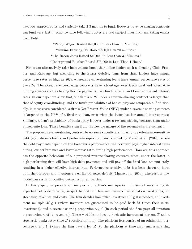
In this paper, we provide an analysis of the firm’s multi-period problem of maximizing its
expected net present value, subject to platform fees and investor participation constraints, for
stochastic revenues and costs. The firm decides how much investment Y ≥ 0 is needed, an invest-
ment multiple M ≥ 1 (where investors are guaranteed to be paid back M times their initial
investment), and a revenue-sharing proportion γ ≥ 0 (in each period the firm pays all investors
a proportion γ of its revenues). These variables induce a stochastic investment horizon T and a
stochastic bankruptcy time B (possibly infinite). The platform fees consist of an origination per-
centage α ∈ [0,1] (where the firm pays a fee αY to the platform at time zero) and a servicing

Author: Crowdfunding via Revenue-Sharing Contracts4
percentage β ∈ [0,1] (where in each period the firm pays a β percent of all investor revenue pay-
ments to the platform). We design a stochastic programming formulation of the firm’s problem,
which is a rather intractable model.
Since the stochastic model is difficult to analyze, we derive a deterministic approximation model
for it, in which we use a cash buffer to cope with uncertainties. We then solve the approximation
problem analytically, which provides generalizable insights. We also solve our stochastic model
numerically using Monte Carlo simulation and a grid-based optimization framework, for serially
correlated random cash-flows that are parameterized using real data from Bolstr. We then compare
the NPVs of the approximate and optimal solutions in the true stochastic model. We conclude
that our approximation provides high quality solutions: the worst-case average error of the approx-
imation solution’s NPV, over all feasible Bolstr campaigns for all levels of cash-flow uncertainty, is
approximately 0.2%.
Finally, we compare the performance of the proposed revenue-sharing contract with equity crowd-
funding and fixed-rate loans, and we identify which type of financing results in a higher NPV or a
lower chance of bankruptcy for a firm; we find that the revenue-sharing contract is superior in most
cases. We next provide a literature review to appropriately position our paper’s contributions.
1.1. Literature Review
There are many papers that study other crowdfunding models, papers that study various aspects
of the interface of operations and finance, as well as a vast literature on revenue-sharing contracts,
primarily in the areas of supply chain management and educational financing. In this section, we
survey the most relevant results in these three streams. However, to the best of our knowledge,
there are no studies investigating crowdfunding via revenue-sharing contracts, except Fatehi and
Wagner (2017), which is a book chapter summary of a preliminary version of this research. Thus,
our research uniquely lies at the intersection of these two literature streams.
Babich et al. (2017) provided a detailed study on how crowdfunding impacts the financing
decisions of entrepreneurs, banks, and venture capital investors. Chen et al. (2017) considered
fundraising success in crowdfunding and studied the optimal referring policies by entrepreneurs,
empirically and analytically. Chakraborty and Swinney (2016) studied how entrepreneurs can signal
their product’s quality to contributors via campaign design in reward-based crowdfunding. Zhang
and Liu (2012) studied a data set from Prosper, focusing on a study of herding behavior in microloan
markets. Lin and Viswanathan (2015) also analyzed data from Prosper and studied the “home
bias” in crowdfunding markets. Iyer et al. (2015) also studied a dataset from Prosper and showed
that lenders use standard information along with nonstandard, or soft, information to evaluate
borrower creditworthiness. Belleflamme et al. (2014) compared two forms of crowdfunding, profit

Author: Crowdfunding via Revenue-Sharing Contracts5
sharing and pre-ordering of products, and showed that if the firm’s investment goal is relatively
high with respect to the market size, then the firm prefers profit-sharing crowdfunding. Finally,
Wei and Lin (2016) study, both theoretically and empirically, the difference between auctions and
posted prices on Prosper.com.
Our paper is also relevant to the literature on the interface of operations and finance. In par-
ticular, our research is relevant to operational financing. There can be many sources of financing,
including traditional bank financing, as well as more novel arrangements that have been attracting
attention in the OM literature, such as buyer financing (Deng et al. 2018) or supplier trade credits
(Lee et al. 2017) or both (Kouvelis and Zhao 2017). We identify crowdfunding as an additional
source of financing, and while we focus on revenue-sharing crowdfunding, we also consider equity
crowdfunding.
The structure of our crowdfunding contracts, revenue-sharing, has also been extensively studied
in the supply chain management literature. However, the combination with financial aspects is
limited. Kouvelis and Zhao (2015) studied contract design for a supply chain with one supplier
and one retailer in the presence of financial constraints and bankruptcy costs, and they show that
a revenue-sharing contract can still coordinate the supply chain. Kouvelis et al. (2017) showed
that revenue-sharing contracts can achieve high efficiency in the presence of cost uncertainty and
working capital constraints. Similarly, we show that a firm can benefit significantly from revenue-
sharing contracts under stochastic cash flows.
Revenue sharing contracts have also appeared in the education field, as a novel approach to
funding students. Nerlove (1975) studied an income-contingent loan program for the financing of
education, which was originally proposed by Friedman and Kuznets (1945) for professional eduction
and by Friedman (1955) for vocational education. One example of such a loan program is the
Yale Tuition Postponement Option, which started in 1971, but was discontinued in 1978 (Ladine
2001). Another example is the Pay-it-Forward plan in Oregon: in 2013, state legislators proposed a
program in which students could attend public colleges without paying tuition, and in return they
would pay 3% percent of their future income to the state for several years after graduation (Palacios
and Kelly 2014). Similarly, the Back-a-Boiler program at Purdue University, which started in Fall
2016 and has already raised $2.2 million, provides funds to undergraduate students to finance their
education through an Income Share Agreement in which students agree to pay a percentage of
their future income over a standard payment term (Purdue 2016). The results and insights of our
paper can also be applied to these student loan agreements.
1.2. Contributions
The contributions of our paper are as follows:
Author: Crowdfunding via Revenue-Sharing Contracts6
1. We are the first, to our knowledge, to study a new emergent model of crowdfunding pioneered
by Bolstr, Localstake, and Startwise. Furthermore, our models are parameterized using real data
from 56 Bolstr campaigns.
2. We study a firm’s expected NPV maximization problem under a revenue-sharing contract,
which is an intractable stochastic model. To overcome the technical difficulties, we design a tractable
deterministic approximation model, in which we use a cash buffer to cope with cash-flow uncertain-
ties. We solve the approximation model analytically, which provides qualitative insights. Numer-
ical experiments, calibrated on real Bolstr data, indicate that the approximation solutions, when
inserted into the true stochastic model, result in an expected NPV that is within 0.2% of the true
optimal NPV, on average. Furthermore, the approximation solutions result in almost the same
bankruptcy probabilities as the optimal stochastic solutions.
3. Our results provide managerial guidelines for the firm; for instance:
(a) A firm can attain a higher NPV and a comparable probability of bankruptcy under
a revenue-sharing contract than under equity crowdfunding. We show that the NPV benefit of
revenue-sharing increases as the firm’s cashflow volatility increases.
(b) A firm can attain a higher NPV and a lower probability of bankruptcy under a revenue-
sharing contract than under a more traditional fixed-rate loan. We also show that these benefits
are more significant for firms with higher levels of cash-flow uncertainty. Intuitively, these benefits
are due to the more flexible nature of the revenue-sharing contract.
(c) As cash-flow uncertainty increases, the optimal investment amount increases, the revenue-
sharing percentage decreases, resulting in a stochastically larger investment horizon (e.g., larger
mean and variance). However, the firm’s maximized NPV is rather insensitive to cash-flow uncer-
tainty. Thus, while the details of the optimal revenue-sharing contract can change considerably
with cash-flow uncertainty, the bottom line NPV is rather robust to this uncertainty.
2. Stochastic Model of Firm
In this section we detail our basic stochastic model of a firm, whose revenue and cost in time
period t, Rt ≥ 0 and Ct ≥ 0, are random variables; we model these cashflows using random walks
with drift, which is explained in detail in Section 2.2. Many firms on Bolstr, Localstake, and
Starwise have raised money to upgrade their existing stores, build a store in a new location, buy
new equipment, and create/upgrade their websites. Due to this expansion, the firm has cash-flow
shortages for a limited time and therefore needs to raise capital, in the amount of Y ≥ 0 (e.g.
dollars), via an intermediary platform that pairs interested individual investors that are willing to
invest. Therefore, the investment Y is a buffer to avoid a negative cash flow.
The investors do not receive equity in the firm, but are paid back, with interest, via a revenue-
sharing contract: at the end of each time period t, the firm is contractually obligated to pay out to

Author: Crowdfunding via Revenue-Sharing Contracts7
all investors a proportion γ ≥ 0 of its revenues for that time period. These payments continue until
each investor receives a multiple M ≥ 1 of his/her initial investment, which occurs at time t= T
(for all investors); this definition of M is motivated by practical implementations (e.g., Bolstr,
Localstake, and Startwise). Note that the investment payments are not fixed, since they depend
on firm revenues, which can vary. The contract’s duration is therefore the stochastic stopping time
T = min
T ≥ 1 :T∑t=1
γRt ≥MY
, (1)
which captures the firm’s contractual obligation to pay γ percent of its revenue to investors until a
total nominal amount of MY has been paid. Time period t= 0 is the initialization of the revenue-
sharing contract when the firm receives total investment Y . The firm must also pay the platform 1)
an origination fee of α∈ [0,1] percent of the total amount raised Y at time t= 0 and 2) a servicing
fee of β ∈ [0,1] percent of all revenue payments made to investors at times t > 0.
We next discuss cash flows, and, for simplicity, we assume the risk-free interest rate is zero (i.e.,
cash does not earn interest). If, in period t, Rt − Ct < 0, there is a cash shortfall; however, this
can potentially be addressed using an excess of cash from previous periods. Thus, we focus on
cumulative cash flows. If there exists τ ≥ 1 such thatτ∑t=1
(Rt −Ct)< 0, then the firm needs cash
in month τ . The firm’s cumulative cash flow at the end of month τ = 1, . . . , T , during the revenue
sharing contract, is∑τ
t=1(Rt−Ct) + (1−α)Y − (β+ 1)γ∑τ
t=1Rt; if τ > T , after the completion of
the contract, the cumulative cash flow is∑τ
t=1(Rt−Ct) + (1−α)Y − (β+ 1)γ∑T
t=1Rt. These two
scenarios can be combined into one expression for the cash flow in period τ ≥ 1:∑τ
t=1(Rt−Ct) +
(1−α)Y − (β+ 1)γ∑min{τ,T}
t=1 Rt.
Due to the stochasticity of the firm’s cash flows, the firm can potentially go bankrupt, for any
combination of contractual parameters (Y,M,γ). Babich and Tang (2016) and Uhrig-Homburg
(2005) model bankruptcy as occurring during the first period where the firm is cash-flow negative;
we adopt this approach. Letting B denote the time period where the firm goes bankrupt, we model
B as a stochastic stopping time (that depends on the stochastic stopping time T ):
B = min
B ≥ 1 :B∑t=1
(Rt−Ct) + (1−α)Y − (β+ 1)γ
min{B,T}∑t=1
Rt < 0
. (2)
The platform and investors receive their payments at the end of each month if the borrower is
not bankrupt; thus, the revenue sharing contract is in effect for τ = 1, . . . ,min{B,T}. As costs and
revenues are stochastic, a risk-neutral firm wants to maximize the firm’s expected NPV
E
[B∑t=1
Rt−Ct(1 + rt)t
]− (β+ 1)γE
[min{B,T}∑
t=1
Rt(1 + rt)t
]+ (1−α)Y, (3)

Author: Crowdfunding via Revenue-Sharing Contracts8
where γE[∑min{B,T}
t=1Rt
(1+rt)t
]is the expected NPV of all payments made to investors,
βγE[∑min{B,T}
t=1Rt
(1+rt)t
]is the expected NPV of all servicing fees paid to the platform, αY is the
origination fee paid to the platform at time t= 0, and, in period t, risk is quantified via imputed
discount rates rt (Arrow and Lind 1978). We assume these discount rates are known. According
to Pratt et al. (2014), small-sized firms can estimate their NPV by using the cost of capital as the
discount rate. Alternatively, Wei and Lin (2016) assume that firms determine their discount rate
according to the lowest interest rate offered to them from other financial institutions.
Finally, we consider the investors. We assume that there is a large pool of investors and the target
investment is raised by n investors, where investor i invests an amount yi ∈ (0, Y ], and∑n
i=1 yi = Y .
We model the investor participation constraints as
E
[min{B,T}∑
t=1
yiY
γRt(1 + δt)t
− yi]≥Ai, i= 1, ..., n, (4)
where yiY
is the fraction of the total payment γRt investor i receives in period t, δt is the discount
rate of investors in period t, the left-hand-side is the investor’s expected NPV, and Ai ≥ 0 is
the target rate of return, in NPV terms, for investor i. In other words, Ai captures investor i’s
opportunity cost of alternative investments. We simplify the constraints in Expression (4) to the
following single constraint
E
[min{B,T}∑
t=1
γ
Y
Rt(1 + δt)t
]≥ max
1≤i≤n
{Aiyi
}+ 1. (5)
The firm is able to select the investment amount Y , the multiple M , and the revenue-sharing
proportion γ in order to maximize its expected NPV. The above analysis results in the firm’s
problem:
zF = maxY,M,γ
E
[B∑t=1
Rt−Ct(1 + rt)t
]− (β+ 1)γE
[min{B,T}∑
t=1
Rt(1 + rt)t
]+ (1−α)Y
s.t. T = min
T ≥ 1 :T∑t=1
γRt ≥MY
(contractual obligation)
B = min
B ≥ 1 :B∑t=1
(Rt−Ct) + (1−α)Y − (β+ 1)γ
min{B,T}∑t=1
Rt < 0
(bankruptcy definition)
E
[min{B,T}∑
t=1
γ
Y
Rt(1 + δt)t
]≥ max
1≤i≤n
{Aiyi
}+ 1 (investor participation)
Y,γ ≥ 0,M ≥ 1.(6)
Table 2, in the appendix, summarizes the main problem parameters and firm variables.

Author: Crowdfunding via Revenue-Sharing Contracts9
2.1. Model Parameterization Using Data from Bolstr.com
We have collected cost and revenue projections from 56 campaigns on the Bolstr platform, and
performed regression analyses on them. The R2 values for the cost regressions ranged from 0.595
to 0.995, with a mean of 0.905 and a standard deviation of 0.079. The R2 values for the rev-
enue regressions ranged from 0.725 to 0.995, with a mean of 0.922 and a standard deviation of
0.065. Therefore, the Bolstr data suggest that linear models of cost and revenue projections, in
expectation, are reasonable assumptions.
We denote a and b as the intercept and slope of a generic revenue regression line, respectively;
similarly, we denote c and d as the intercept and slope of an arbitrary cost regression line, respec-
tively. Letting E[Rt] and E[Ct] denote the expected revenue and cost in period t, respectively, we
assign
E[Rt] = a+ bt and E[Ct] = c+ dt. (7)
Many, but not all, of our results will utilize the linearity of cash flows.
2.2. Modeling Cashflows
Motivated by the cash flow models in Dechow et al. (1998), we generate revenues (R1,R2, . . .) and
costs (C1,C2, . . .) using random walk processes:
Rt =Rt−1 +Zrt and Ct =Ct−1 +Zct , t≥ 1, (8)
where R0 = a and C0 = c are given in Equation (7). The Zrt are independent normal random
variables with common mean µr = b, where b is given by Equation (7), and standard deviation
σr = µr/k, where k is a tunable parameter. Similarly, Zct are independent normal random variables
with common mean µc = d, where d is given by Equation (7), and standard deviation σc = µc/k.
The means can be easily calculated: E[Rt] = a+ bt and E[Ct] = c+dt, in agreement with Equation
(7). Furthermore, the random walk model exhibits serial correlation: it is straightforward to show
that, for s < t, cov(Rs,Rt) = s(σr)2 and cov(Cs,Ct) = s(σc)2. Note that Brownian motion is a limit
of a random walk process (Kac 1947). Therefore, our proposed random walk models for revenues
and costs can be considered as approximate Brownian motion processes with drifts µr and µc and
volatilities σr and σc, respectively (Ross 1996, Sigman 2006).
2.3. Analysis Roadmap
We found an analytical solution to Problem (6) to be intractable. In the next section, we derive an
approximation for the stochastic problem. The approximation problem is a deterministic relaxation
where σr = σc = 0, but we add a cash-flow buffer to the bankruptcy definition to deal with cash-flow
uncertainties in the stochastic model; in this case, we are able to derive analytical solutions that

Author: Crowdfunding via Revenue-Sharing Contracts10
provide generalizable insights. These results are provided in Section 3. To evaluate the quality of
our approximation, we also solve Problem (6) for real Bolstr data, using Monte Carlo simulation,
to determine the stochastic stopping times (B,T ) and expectations, combined with numerical
optimization on a fine grid of (Y,M,γ) space. We utilize random walks with drift for the cash flows,
where σr = µr/k and σc = µc/k for various values of k; this analysis can be found in Section 4.
Finally, in Sections 5–6, we show that the revenue-sharing contract compares favorably with equity
crowdfunding and fixed-rate loans, respectively.
3. Deterministic Approximation to Stochastic Model
In this section, we consider a deterministic approximation to Problem (6) where the cash flows Rt
and Ct are known exactly. This simplification results in the conversion of the bankruptcy time B
and investment duration T into parameters, rather than random variables. We assume, given that
cash flows are known exactly, the firm desires to avoid bankruptcy. Thus, reversing the condition
for bankruptcy in Equation (2), we introduce constraints that require the firm to be cash-flow
positive above θ ≥ 0, for all time periods τ ≥ 1, where θ is a cash buffer to account for cash-flow
uncertainties in the stochastic problem:
τ∑t=1
(Rt−Ct) + (1−α)Y − (β+ 1)γ
min{τ,T}∑t=1
Rt ≥ θ, τ ≥ 1. (9)
Similarly, in project management, Long and Ohsato (2008) developed a deterministic schedule
and used a project buffer for dealing with resource uncertainty. They determined the size of the
buffer numerically; similarly, in Section 4.2 we determine the size of the cash-buffer θ numerically
as a function of problem data. We show that as the uncertainty of revenues and costs increases,
θ should increase to make the deterministic approximation solution feasible for the stochastic
problem and provide a high quality approximation for the stochastic problem.
These constraints imply that B =∞ as the firm will never go bankrupt. In Section 4 we show,
via computational experiments, that the optimal solution to the stochastic model in Problem (6)
induces a low probability of firm bankruptcy over feasible Bolstr campaigns, which suggests that
the constraints in (9) are unlikely to eliminate the optimal solution to the stochastic model; in
Section 4.2 we evaluate the approximation quality of the deterministic model developed in this
section for Problem (6), with very encouraging results.
Next, since the variables Y , M , and γ are continuous, we assume that the definition of T in
Equation (1) holds exactly and deterministically:
T∑t=1
γRt =MY. (10)

Author: Crowdfunding via Revenue-Sharing Contracts11
These simplifications result in a deterministic approximation to Problem (6), parameterized by
the investment duration T :
zF (T ) = maxY,M,γ
∞∑t=1
Rt−Ct(1 + rt)t
− (β+ 1)γT∑t=1
Rt(1 + rt)t
+ (1−α)Y
s.t.T∑t=1
γRt =MY (contractual obligation)
τ∑t=1
(Rt−Ct) + (1−α)Y − (β+ 1)γ
min{τ,T}∑t=1
Rt ≥ θ, τ ≥ 1 (cash-flow constraints)
T∑t=1
γ
Y
Rt(1 + δt)t
≥ max1≤i≤n
{Aiyi
}+ 1 (investor participation)
Y,γ ≥ 0,M ≥ 1.(11)
3.1. Analysis for fixed T ∈NIn this subsection, we solve Model (11) for a fixed T ∈N. To begin our analysis, we point out some
simplifications. First, we let A = max1≤i≤n
{Aiyi
}to simplify the exposition. Second, the contractual
obligation constraint can be used to solve for γ = MY∑Tt=1Rt
, and γ is eliminated as a variable. In the
subsequent analysis, it will be convenient to define the set
X ,
{τ ∈N :
τ∑t=1
(Rt−Ct)< θ}, (12)
which indexes all the time periods where the firm, without any investment, has cash flow below θ.
It is also convenient to define the parameters Zτ (T ), which depend only on firm problem data and
T :
Zτ (T ), (A+ 1)(β+ 1)
∑min{τ,T}t=1 Rt∑T
t=1Rt
(1+δt)t
− (1−α). (13)
The resulting model has the following solution.
Proposition 1. Problem (11), with T ∈ N fixed and X 6= ∅, is feasible if and only if Zτ (T )<
0, ∀τ ∈X and maxτ∈X
{∑τt=1(Rt−Ct)−θ
Zτ (T )
}≤min τ 6∈X
Zτ (T )>0
{∑τt=1(Rt−Ct)−θ
Zτ (T )
}, and has the optimal solu-
tion M∗(T ) =(A+1)
∑Tt=1Rt∑T
t=1Rt
(1+δt)t
and γ∗(T ) = (A+1)Y ∗(T )∑Tt=1
Rt(1+δt)
t
,
where
• if (β+1)(A+1)
∑Tt=1
Rt(1+rt)
t∑Tt=1
Rt(1+δt)
t
−(1−α)≥ 0, then Y ∗(T ) = maxτ∈X
{∑τt=1(Rt−Ct)−θ
Zτ (T )
}; alternatively,
if X = ∅, then Y ∗ = 0, γ∗ = 0, and M∗ = 1 for all T ∈N.
• if (β+ 1)(A+ 1)
∑Tt=1
Rt(1+rt)
t∑Tt=1
Rt(1+δt)
t
− (1−α)< 0, then Y ∗(T ) = min τ 6∈XZτ (T )>0
{∑τt=1(Rt−Ct)−θ
Zτ (T )
}; alterna-
tively, if X = ∅, then Y ∗(T ) = minτ∈N
Zτ (T )>0
{∑τ
t=1(Rt−Ct)− θZτ (T )
}for all T ∈N.
The maximized NPV is zF (T ) =∑∞
t=1Rt−Ct(1+rt)t
−(
(β+ 1)(A+ 1)
∑Tt=1
Rt(1+rt)
t∑Tt=1
Rt(1+δt)
t
− (1−α)
)Y ∗(T ).

Author: Crowdfunding via Revenue-Sharing Contracts12
Note that Proposition 1 only requires that the cash flows Rt and Ct be deterministic, but does
not require them to be linear. The feasibility constraints in Proposition 1 can be interpreted as
financial conditions where the firm can eventually survive on its own; as an example where this is
not possible, consider the case where Ct >Rt for all t. In particular, Zτ (T )< 0, ∀τ ∈X ensures that
the firm is cash-flow positive for all periods τ ∈X, due to the investment Y ∗(T ), and the condition
Y ∗(T )≤min τ 6∈XZτ (T )>0
{∑τt=1(Rt−Ct)−θ
Zτ (T )
}ensures that the firm can afford to pay back M∗(T )Y ∗(T ) to
investors and βM∗(T )Y ∗(T ) to the platform.
If the firm’s discount rates rt are not too large, relative to the investors’ discount rates δt, and
(β+ 1)(A+ 1)
∑Tt=1
Rt(1+rt)
t∑Tt=1
Rt(1+δt)
t
− (1−α)≥ 0 holds, then we see that, intuitively, if X = ∅, then the firm
does not need any investment and Y ∗(T ) = 0. Alternatively, if X 6= ∅ and the feasibility conditions
are satisfied, then
((β+ 1)(A+ 1)
∑Tt=1
Rt(1+rt)
t∑Tt=1
Rt(1+δt)
t
− (1−α)
)Y ∗(T ) can be interpreted as the firm’s cost
for avoiding bankruptcy.
Alternatively, if (β + 1)(A + 1)
∑Tt=1
Rt(1+rt)
t∑Tt=1
Rt(1+δt)
t
− (1 − α) < 0, then the firm’s discount rates rt are
relatively larger than the investors’ discount rates δt. Therefore the firm’s gain from the (1−α)Y
investment at time zero is greater than the firm’s NPV of future payments to the investors and
the platform. As a result, the firm benefits by raising a larger investment.
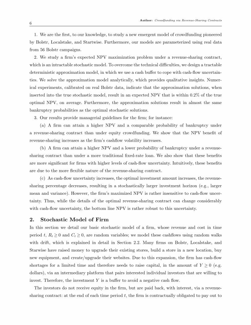
In Figure 1 we plot the average of the objective function value zF (T ) and the average of the
optimal variables (Y ∗(T ),M∗(T ), γ∗(T )) from Proposition 1 as a function of T , over feasible Bolstr
campaigns, for the following parameter set: For each campaign we let linear revenues Rt =E[Rt]
and costs Ct = E[Ct], where E[Rt] and E[Ct] are given in Equation (7) and only use the given
campaign’s data, θ = 0, α = 0.05 and β = 0.01 (per a Bolstr memorandum), A= 0.1 (i.e., a 10%
NPV return for investors), and rt = δt = 0.01, ∀t (the discount rate per period, typically a month).
These results are useful in the sequel for interpreting the results for the stochastic problem where
the level of variability in costs and revenues is small.
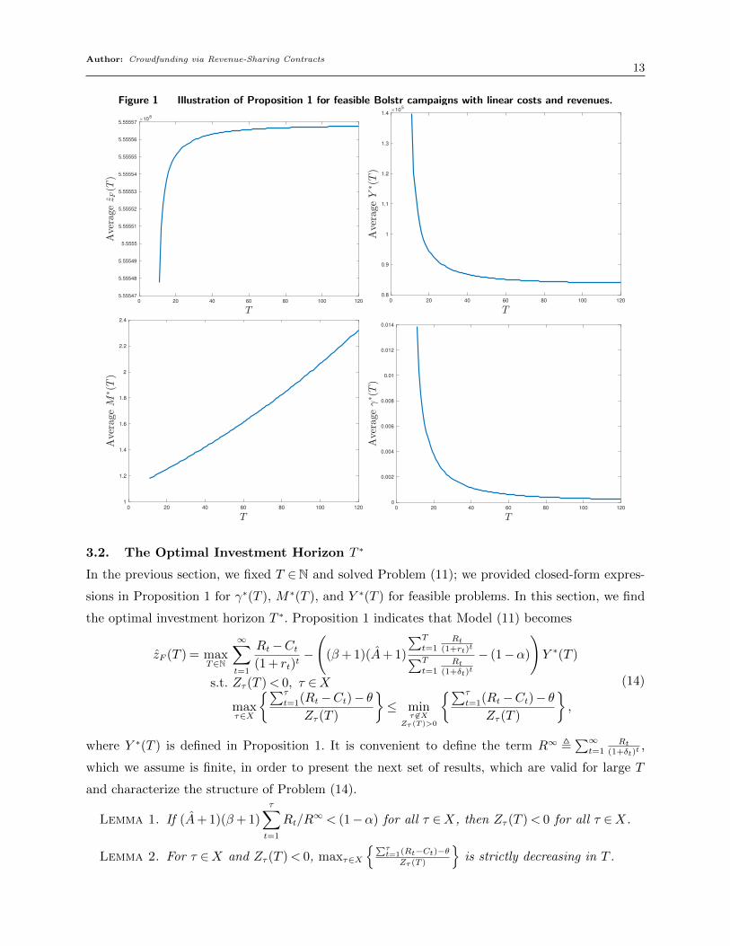
The plot on the top left of Figure 1 suggests that zF (T ) converges rather quickly to an asymptote.
In the next section, for linear cash-flows, we derive conditions for which maxT
zF (T ) is attained
when T →∞. However, our numerical results suggest that relatively small values of T , say T ∈{18, . . . ,30}, suffice to attain almost all the potential value of max
TzF (T ). In the top right plot, we
observe that Y ∗(T ) decreases rather quickly to an asymptote as well. In the bottom left plot we
see that M∗(T ) is increasing in T and in the bottom right plot we see that γ∗(T ) is decreasing in
T , which intuitively align with the increased investment duration T . We point out that our model
was only feasible for T ≥ 12 for all feasible campaigns for θ= 0; in the next section, for linear cash
flows, we provide a rigorous proof that Problem (11) can only be feasible for large enough T .
Author: Crowdfunding via Revenue-Sharing Contracts13
Figure 1 Illustration of Proposition 1 for feasible Bolstr campaigns with linear costs and revenues.
0 20 40 60 80 100 120
5.55547
5.55548
5.55549
5.5555
5.55551
5.55552
5.55553
5.55554
5.55555
5.55556
5.5555710
8
0 20 40 60 80 100 120
0.8
0.9
1
1.1
1.2
1.3
1.410
5
0 20 40 60 80 100 120
1
1.2
1.4
1.6
1.8
2
2.2
2.4
0 20 40 60 80 100 120
0
0.002
0.004
0.006
0.008
0.01
0.012
0.014
3.2. The Optimal Investment Horizon T ∗
In the previous section, we fixed T ∈N and solved Problem (11); we provided closed-form expres-
sions in Proposition 1 for γ∗(T ), M∗(T ), and Y ∗(T ) for feasible problems. In this section, we find
the optimal investment horizon T ∗. Proposition 1 indicates that Model (11) becomes
zF (T ) = maxT∈N
∞∑t=1
Rt−Ct(1 + rt)t
−(
(β+ 1)(A+ 1)
∑T
t=1Rt
(1+rt)t∑T
t=1Rt
(1+δt)t
− (1−α)
)Y ∗(T )
s.t. Zτ (T )< 0, τ ∈Xmaxτ∈X
{∑τ
t=1(Rt−Ct)− θZτ (T )
}≤ min
τ 6∈XZτ (T )>0
{∑τ
t=1(Rt−Ct)− θZτ (T )
},
(14)
where Y ∗(T ) is defined in Proposition 1. It is convenient to define the term R∞ ,∑∞
t=1Rt
(1+δt)t,
which we assume is finite, in order to present the next set of results, which are valid for large T
and characterize the structure of Problem (14).
Lemma 1. If (A+ 1)(β+ 1)τ∑t=1
Rt/R∞ < (1−α) for all τ ∈X, then Zτ (T )< 0 for all τ ∈X.
Lemma 2. For τ ∈X and Zτ (T )< 0, maxτ∈X
{∑τt=1(Rt−Ct)−θ
Zτ (T )
}is strictly decreasing in T .

Author: Crowdfunding via Revenue-Sharing Contracts14
Lemma 3. For τ 6∈X and Zτ (T )> 0, min τ 6∈XZτ (T )>0
{∑τt=1(Rt−Ct)−θ
Zτ (T )
}is strictly increasing in T .
The next lemma builds upon Lemmas 2–3 to characterize the objective function of Problem (14).
Lemma 4. If rt = r ≥ δ = δt,∀t or rt = δt,∀t, then the objective function of Problem (14) is
increasing in T , for large T .
Lemmas 2 and 3 suggest that maxτ∈X
{∑τ
t=1(Rt−Ct)− θZτ (T )
}≤ min
τ 6∈XZτ (T )>0
{∑τ
t=1(Rt−Ct)− θZτ (T )
}is
attained asymptotically. However, this is not always possible. Consider the following example.
Example 1. Let the revenues Rt = 10 for t ≥ 1 and the costs are C1 = 15, C2 = 5, and
Ct = 10 for t ≥ 3, and θ = 0. The set X = {1} and, for feasible values of (A,α,β, δt),
maxτ∈X
{∑τ
t=1(Rt−Ct)− θZτ (T )
}> 0 for all feasible T . In contrast,
∑τ
t=1(Rt − Ct) = 0 for all τ 6∈ X,
implying minτ 6∈X
Zτ (T )>0
{∑τ
t=1(Rt−Ct)− θZτ (T )
}= 0.
In the next subsection, we see that an assumption of linear cash flows resolves the issue encoun-
tered in the above counterexample, and Problem (14) is solvable analytically. Recall that the
linearity of revenues and costs are supported by real data from Bolstr, as explained in Section 2.1.
3.2.1. Linear Firm Costs and Revenues In this subsection, we consider Problem (14) when
the costs and revenues are linear: Rt = a+ bt and Ct = c+dt. We could, for instance, parameterize
(a, b, c, d) using the regression analysis on Bolstr data. The set X, for linear costs and revenues,
simplifies to
X =
{τ ∈N : (a− c)τ + (b− d)
τ(τ + 1)
2< θ
}. (15)
The following function is useful for the subsequent analysis and results:
f(τ),
τ∑t=1
(Rt−Ct)− θ
Zτ (T )=
(a− c)τ + (b− d)τ(τ + 1)
2− θ
η(T )(aτ + b τ(τ+1)
2
)− (1−α)
, (16)
where η(T ) , (A+1)(β+1)∑Tt=1
Rt(1+δt)
t
> 0. This function allows us to write maxτ∈X
{∑τt=1(Rt−Ct)−θ
Zτ (T )
}=
maxτ∈X f(τ) and min τ 6∈XZτ (T )>0
{∑τt=1(Rt−Ct)−θ
Zτ (T )
}= min τ 6∈X
Zτ (T )>0f(τ), where max
τ∈Xf(τ) is a lower bound
on Y ∗(T ) to allow cash-flow positivity at or above θ and min τ 6∈XZτ (T )>0
f(τ) is an upper bound on
Y ∗(T ) to ensure that the firm can afford to pay back M∗(T )Y ∗(T ) to investors and βM∗(T )Y ∗(T )
to the platform. Our next two results characterize the cases where the set X is unbounded or
empty, which results in infeasible and trivial firm optimization problems, respectively.
Lemma 5. If 1) b < d or 2) b= d and a< c+ θ, then Problem (14) is infeasible.
Under the conditions of Lemma 5, the firm will eventually go bankrupt for all values of (Y,M,γ).

Author: Crowdfunding via Revenue-Sharing Contracts15
Figure 2 The form of the function f(τ).
50 100 150 200 2500
500
1000
1500
2000
2500
3000
3500
4000
4500
5000
τ
f(τ
)
f (τ ), for τ ∈ X
f (τ ), for τ 6∈ X andZτ (T ) > 0
Lemma 6. If 1) b > d and (b− d)≥ (c− a) + θ and (β+ 1)(A+ 1)
∑Tt=1
Rt(1+rt)
t∑Tt=1
Rt(1+δt)
t
− (1−α)≥ 0 or 2)
b= d and a≥ c+ θ, then Y ∗(T ) = 0 for all T ∈N in Problem (11).
Under either of the conditions of Lemma 6, the firm does not need any outside funding and is
cash-flow positive at or above θ for all periods τ ≥ 1.
Another set of conditions where the firm is cash-flow positive at or above θ for all periods τ ≥ 1
is b > d and b− d≥ (c− a) + θ and (β+ 1)(A+ 1)
∑Tt=1
Rt(1+rt)
t∑Tt=1
Rt(1+δt)
t
− (1−α)< 0. In the next lemma, we
show that under these conditions, if feasible, the firm borrows money from investors although it is
already cash-flow positive at or above θ. The reason is that, under these conditions, the firm’s gain
from raising an investment at time t= 0 is larger than the NPV of its future monthly payments to
the investors and the platform, due to its high discount rates.
Lemma 7. If b > d and b− d≥ (c− a) + θ and (β+ 1)(A+ 1)
∑Tt=1
Rt(1+rt)
t∑Tt=1
Rt(1+δt)
t
− (1−α)< 0, then for
θ≤ θL(T ), where θL(T ) is a function of T and problem parameters, we have for all T ∈N:
• if cb− da≥ 0, then Y ∗(T ) = min{f(bτ ∗∗c), f(dτ ∗∗e)}, where τ ∗∗ is real and equal to
τ∗∗ =(1−α)(b− d)− η(T )θb+
√((1−α)(b− d)− η(T )θb)
2− η(T )(cb− da) ((2(c− a)− (b− d))(1−α) + η(T )θ(2a+ b))
(cb− da)η(T ).
• if cb− da< 0, then Y ∗(T ) = (b− d)/η(T )b.
We have characterized all combinations of (a, b, c, d), except the case where b > d and b− d <(c− a) + θ. We break this case into two sub-cases: i) b > d and b− d < (c− a) + θ and cb > da,
and ii) b > d and b− d < (c− a) + θ and cb≤ da. These cases result in Problem (14) being feasible
with a non-trivial solution. In particular, Case i includes firms that have cash-flow shortages for
a limited time, but have expectations of positive cash flows in the future. Case ii includes firms

Author: Crowdfunding via Revenue-Sharing Contracts16
that have positive cash flows, but they are below θ, and the firm receives investment to increase its
cash flow to at least θ. Recall that θ is a cash buffer in the deterministic approximation problem
to account for cash-flow uncertainties in the stochastic problem. We begin by characterizing the
set X for both these cases.
Lemma 8. If b > d and b − d < (c − a) + θ, then X ={τ ∈N : 1≤ τ < (c−a− b−d2 )+
√(c−a− b−d2 )
2+2θ(b−d)
b−d
}.
From the set X it is clear that as θ increases, the number of periods where the firm has a cash
flow below θ increases. The following lemma indicates that the problem is not feasible for θ larger
than a threshold.
Lemma 9. The first constraint in Problem (14), Zτ (T )< 0 for all τ ∈X, is equivalent to the con-
ditions θ≤ θ(T ) and (ad− bc) + (b−d)√
(a+ b/2)2 + 2(1−α)b/η(T )≥ 0, where θ(T ) is a function
of T and problem parameters.
Note that the left-hand side of the second condition in Lemma 9 is increasing in T , albeit
asymptotically, due to η(T ). Therefore, if it is possible for the first constraint of Problem (14) to
hold, it will be feasible for a large enough T and a small enough θ. We next analyze Cases i and ii,
building upon the condition in Lemma 9, to address the second constraint in Problem (14).
Case i: b > d and b− d < (c− a) + θ and cb > da. The next three lemmas characterize the
second constraint in Problem (14) for Case i: b > d and b− d < (c− a) + θ and cb > da, assuming
the feasibility conditions of the first constraint in Lemma 9 hold.
Lemma 10. If b > d, cb > da, and (ad− bc) + (b− d)√
(a+ b/2)2 + 2(1−α)b/η(T )≥ 0, then for
θ≤ θ(T ) and b− d< (c− a) + θ, where θ(T ) is a function of T and problem parameters:
a) If θ≥ ((b−d)−2(c−a))(1−α)η(T )(2a+b)
, then maxτ∈X
f(τ) = max{f(bτ ∗c), f(dτ ∗e)}, where τ ∗ is real and equal to
τ∗ =(1−α)(b− d)− η(T )θb−
√((1−α)(b− d)− η(T )θb)
2− η(T )(cb− da) ((2(c− a)− (b− d))(1−α) + η(T )θ(2a+ b))
(cb− da)η(T ).
b) Otherwise, maxτ∈X
f(τ) =a+ b− c− d− θ
η(T )(a+ b)− (1−α).
Lemma 11. If b > d, cb > da, and (ad− bc) + (b− d)√
(a+ b/2)2 + 2(1−α)b/η(T )≥ 0, then for
θ ≤ θ(T ) and b− d < (c− a) + θ, where θ(T ) is a function of T and problem parameters, we have
minτ 6∈X
Zτ (T )>0
{f(τ)}= min{f(bτ ∗∗c), f(dτ ∗∗e)}, where τ ∗∗ is real and equal to
τ∗∗ =(1−α)(b− d)− η(T )θb+
√((1−α)(b− d)− η(T )θb)
2− η(T )(cb− da) ((2(c− a)− (b− d))(1−α) + η(T )θ(2a+ b))
(cb− da)η(T ).

Author: Crowdfunding via Revenue-Sharing Contracts17
Lemma 12. If b > d, cb > da, and (ad − bc) + (b − d)√
(a+ b/2)2 + 2(1−α)b/η(T ) ≥ 0, then
∃ θ(T ) such that for θ ≤ θ(T ) and b− d < (c− a) + θ, where θ(T ) is a function of T and problem
parameters, the inequality maxτ∈X{f(τ)} ≤ min
τ 6∈XZτ (T )>0
{f(τ)} holds for T large enough.
Lemmas 10 – 12 prove that, for linear cash flows and Case i, if θ is small enough and T is large
enough, Problem (14) is feasible. We next accomplish the same task for Case ii.
Case ii: b > d and b− d < (c− a) + θ and cb ≤ da. The next three lemmas characterize the
second constraint in Problem (14) for Case ii: b > d and b− d < (c− a) + θ and cb≤ da, assuming
the feasibility conditions of the first constraint in Lemma 9 hold.
Lemma 13. If b > d and cb≤ da, and (ad− bc) + (b− d)√
(a+ b/2)2 + 2(1−α)b/η(T )≥ 0, then
for θ ≤ θ(T ) and b− d < (c− a) + θ, where θ(T ) is a function of T and problem parameters, we
have maxτ∈X
f(τ) =a+ b− c− d− θ
η(T )(a+ b)− (1−α).
Lemma 14. If b > d and cb≤ da, and (ad− bc) + (b− d)√
(a+ b/2)2 + 2(1−α)b/η(T )≥ 0, then
for θ ≤ θ(T ) and b− d < (c− a) + θ, where θ(T ) is a function of T and problem parameters, we
have minτ 6∈X
Zτ (T )>0
{f(τ)}= (b− d)/η(T )b.
Note that from b > d and cb≤ da, we conclude a≥ c. Conditions b > d and a≥ c represent a firm
that has higher revenues than costs in all periods, with the revenue growth larger than that of cost;
however, the firm’s cash flow is not above θ in all periods, which drives the need for investment.
Lemma 15. If b > d and cb≤ da, and (ad− bc) + (b− d)√
(a+ b/2)2 + 2(1−α)b/η(T )≥ 0, then
∃ θ(T ) such that for θ ≤ θ(T ) and b− d < (c− a) + θ, where θ(T ) is a function of T and problem
parameters, the inequality maxτ∈X{f(τ)} ≤ min
τ 6∈XZτ (T )>0
{f(τ)} holds.
The conclusion of Lemmas 12 and 15, maxτ∈X{f(τ)} ≤ min
τ 6∈XZτ (T )>0
{f(τ)}, guarantees that the firm
is cash-flow positive at or above θ in all months for Cases i and ii, respectively, which is only
possible if θ is small enough. Lemmas 2 – 3 prove that the inequality maxτ∈X{f(τ)} ≤ min
τ 6∈XZτ (T )>0
{f(τ)},
if feasible, is feasible for T large enough. Thus, Problem (14), under linear cash flows and Cases
i and ii, is feasible for T large enough and θ small enough. The results in Lemmas 7, 10, and
13 provide closed-form solutions for Y ∗(T ) under all non-trivial cases and Proposition 1 provides
closed-form solutions for M∗(T ), and γ∗(T ) as a function of Y ∗(T ). We found that T = 120 worked
well to generate high-quality approximations for problems parameterized by real Bolstr data. These
optimal variables for Problem (14) are used as approximate solutions for the stochastic model in
Problem (6), whose quality we explore in the next section.
To complete the analysis of the deterministic problem, we now collect all these results to solve
Problem (14) for the cases where rt = r≥ δ= δt,∀t or rt = δt,∀t. Proposition 1, and Lemmas 7, 10,

Author: Crowdfunding via Revenue-Sharing Contracts18
and 13 for linear cash flows, provide closed-form solutions for the optimal γ∗(T ), M∗(T ), and Y ∗(T ),
assuming model feasibility and a fixed T ∈N. Lemma 4 indicates that the objective of Problem (14)
is strictly increasing in T . Lemmas 1 – 3 prove that Problem (14), if feasible, is feasible for large
enough T . We also note that limT→∞
η(T ) = limT→∞
(A+ 1)(β+ 1)∑T
t=1(a+bt)
(1+δt)t
= (A+ 1)(β+ 1)/R∞. Lemmas 11 –
12 and 14 – 15 prove, for Cases i and ii, respectively, that for linear cash flows and large enough
T, the model is feasible. Together, these results solve Problem (14) for linear costs and revenues,
which we summarize in the next propositions. Specifically, in Proposition 2 we characterize the
optimal solutions for (β+ 1)(A+ 1)
∑Tt=1
Rt(1+rt)
t∑Tt=1
Rt(1+δt)
t
− (1−α)≥ 0 and in Proposition 3 we do the same
for (β+ 1)(A+ 1)
∑Tt=1
Rt(1+rt)
t∑Tt=1
Rt(1+δt)
t
− (1−α)< 0.
Proposition 2.
For (β + 1)(A+ 1)
∑Tt=1
Rt(1+rt)
t∑Tt=1
Rt(1+δt)
t
− (1− α) ≥ 0 and either rt = r ≥ δ = δt,∀t or rt = δt,∀t, if b > d,
b−d< (c−a) +θ, θ≤ limT→∞
θ(T ), and (ad− bc) + (b−d)√
(a+ b/2)2 + 2(1−α)b R∞
(A+1)(β+1)≥ 0, then
• if cb > da and θ ≥ ((b−d)−2(c−a))(1−α)(A+1)(β+1)
R∞(2a+b), then T ∗ = ∞, M∗ = ∞, Y ∗ =
max{f(bτ ∗c), f(dτ ∗e)}, γ∗ = (A+1)Y ∗
R∞ , where
τ∗ =(1−α)(b− d)− θb(A+ 1)(β+ 1)/R∞
(cb− da)(A+ 1)(β+ 1)/R∞−√(
(1−α)(b− d)− θb(A+ 1)(β+ 1)/R∞)2− (A+ 1)(β+ 1)/R∞(cb− da)
((2(c− a)− (b− d))(1−α) + (A+ 1)(β+ 1)/R∞θ(2a+ b)
)(cb− da)(A+ 1)(β+ 1)/R∞
.
• Otherwise, T ∗ =∞, M∗ =∞, Y ∗ = a+b−c−d−θ(A+1)(β+1)(a+b)/R∞−(1−α) , γ
∗ =(A+1) a+b−c−d−θ
η(T )(a+b)−(1−α)R∞ .
The firm’s maximized NPV is zF =∑∞
t=1a−c+(b−d)t
(1+rt)t−(
(β+ 1)(A+ 1)
∑Tt=1
Rt(1+rt)
t∑Tt=1
Rt(1+δt)
t
− (1−α)
)Y ∗.
Proposition 3.
For (β + 1)(A + 1)
∑Tt=1
Rt(1+rt)
t∑Tt=1
Rt(1+δt)
t
− (1 − α) < 0 and rt = r ≥ δ = δt,∀t, if b > d, b − d ≥ (c − a) +
θ, and θ ≤ limT→∞
θL(T ) or if b > d, b − d < (c − a) + θ, θ ≤ limT→∞
θ(T ), and (ad − bc) + (b −d)√
(a+ b/2)2 + 2(1−α)b R∞
(A+1)(β+1)≥ 0, then
• if cb− da≥ 0, then Y ∗(T ) = min{f(bτ ∗∗c), f(dτ ∗∗e)}• if cb− da< 0, then Y ∗(T ) = (b− d)/η(T )b,
where τ ∗∗ is real and equal to
τ∗∗ =(1−α)(b− d)− θb(A+ 1)(β+ 1)/R∞
(cb− da)(A+ 1)(β+ 1)/R∞+√(
(1−α)(b− d)− θb(A+ 1)(β+ 1)/R∞)2− (A+ 1)(β+ 1)/R∞(cb− da)
((2(c− a)− (b− d))(1−α) + (A+ 1)(β+ 1)/R∞θ(2a+ b)
)(cb− da)(A+ 1)(β+ 1)/R∞
,
and T ∗ = ∞, M∗ = ∞, γ∗ = (A+1)Y ∗
R∞ . The firm’s maximized NPV is zF =∑∞
t=1a−c+(b−d)t
(1+rt)t−(
(β+ 1)(A+ 1)
∑Tt=1
Rt(1+rt)
t∑Tt=1
Rt(1+δt)
t
− (1−α)
)Y ∗.
Author: Crowdfunding via Revenue-Sharing Contracts19
From Propositions 2 and 3, we see that if rt = r ≥ δ = δt,∀t or rt = δt,∀t, then Y ∗ and γ∗
are finite, but M∗ and T ∗ are infinite. This solution corresponds to a financial perpetuity (an
annuity with no termination) with non-fixed payments that are a function of firm revenues. Note
that perpetuities are common in modern business (e.g., anyone can purchase a perpetuity through
Bank of America’s Merrill Edge brokerage). More prominent examples include LeBron James, a
four time NBA MVP, and soccer star David Beckham having lifetime contracts with Nike and
Adidas, respectively (Novy-Williams 2015). Furthermore, Gerber et al. (2012) provides a study of
three crowdfunding platforms and showed that many individuals and firms use crowdfunding to
make direct and long term connections with investors; a perpetuity precisely achieves a long-term
connection.
Our perpetuity solution can also be interpreted as a pseudo type of equity crowdfunding. Ross
et al. (2002) explains that the present value of stock is equivalent to the discounted present value
of all future dividends, which are typically a share of profits (page 198 of O’Sullivan and Sheffrin
(2007)). If we replace profits with revenues, we obtain our perpetuity contract. In Section 5 we
formally study the difference between our model and an equity crowdfunding model that shares
profits, rather than revenues, and we show that the revenue-sharing contract is superior.
4. Analysis of Stochastic Model4.1. Simulation-based Numerical Optimization of Stochastic Model
In order to solve Problem (6), we let revenues Rt and costs Ct of each of the 56 Bolstr campaigns
follow the random walk processes in (8). We set the highest allowable values of σr and σc as µr/3
and µc/3, respectively, so that revenues and costs are non-negative with high probability. More
specifically, we consider σr = µr/k and σc = µc/k for k ∈ {3,4,5,6,7,8,9,10,15}, along with the
additional deterministic case of k→∞.
In our base parameter set, we let rt = δt = 0.01, for all t, α= 0.05, β = 0.01, and A= 0.1 (i.e.,
a 10% NPV return for investors); note that r is the discount rate per period, which is typically a
month and that the choice of α= 0.05 and β = 0.01 is supported by a Bolstr memorandum. Many
online platforms such as Bolstr, LendingClub, and Prosper charge 1% servicing fee for collecting
and processing payments. These online lenders usually charge borrowers origination fees of typically
1%− 8%.
We approximate an infinite horizon by considering t∈ {1, ...,N} where N = 1000; we selected this
value of N so that N >max{B,T} holds with high probability; furthermore, there is no evidence
that revenue-sharing contracts at Bolstr and Localstake last longer than 1000 months, and as
pointed out earlier most Bolstr campaigns last 2-5 years. For analyzing Problem (6) numerically,
we discretized the (Y,M,γ) space. In particular, we considered values of Y ∈ {0,∆Y ,2∆Y , . . . , Y },

Author: Crowdfunding via Revenue-Sharing Contracts20
M ∈ {1,1 + ∆M ,1 + 2∆M , . . . ,M}, and γ ∈ {0,∆γ ,2∆γ , . . . , γ}, where (∆Y ,∆M ,∆γ , Y ,M,γ) =
(5000,0.25,0.01,2000000,3,1) were chosen to balance computational time and solution quality.
For each campaign, we used Monte Carlo simulation to generate m = 1000 realizations of
the (R1, . . . ,RN) and (C1, . . . ,CN) vectors, which allowed us to generate m realizations of the
T and B random variables for each (Y,M,γ) tuple in the discretized set. Then, for each vari-
able tuple, averaging over the m trials, we estimate E(∑B
t=1Rt−Ct(1+r)t
), E
(∑min{B,T}t=1
Rt(1+r)t
), and
E(∑min{B,T}
t=1Rt
(1+δ)t
), which allowed us to evaluate the feasibility of the variable tuple. Finally, we
evaluated the objective function for each feasible (Y,M,γ) tuple and chose the one that maximizes
the objective function as the optimal solution. Depending on the standard deviations, 90-95% of
the 56 Bolstr campaigns were feasible.
4.2. Evaluation of Deterministic Approximation in Section 3
In this subsection, we evaluate the value of the approximate Problem (14) with respect to that
of the stochastic Problem (6), for T large enough. For the numerical results presented below, we
consider T = 120, though the performance is insensitive for larger T . In Section 4.3 we show that if
we use the approximation solutions in the true stochastic model, the expected investment horizon
T is close to the choice of T = 120. The main parameters that we vary for each campaign are
the standard deviations σr and σc; all other problem parameters are listed above. As mentioned
previously, we consider σr ∈ [0, µr/3] and σc ∈ [0, µc/3], so that revenues and costs are non-negative
with high probability.
For each level of variability, we find the optimal θ ∈ [0,2M ] which makes the approximation
solutions (Y ∗(θ),M∗(θ), γ∗(θ)) feasible for Problem (6) and results in the minimum approximation
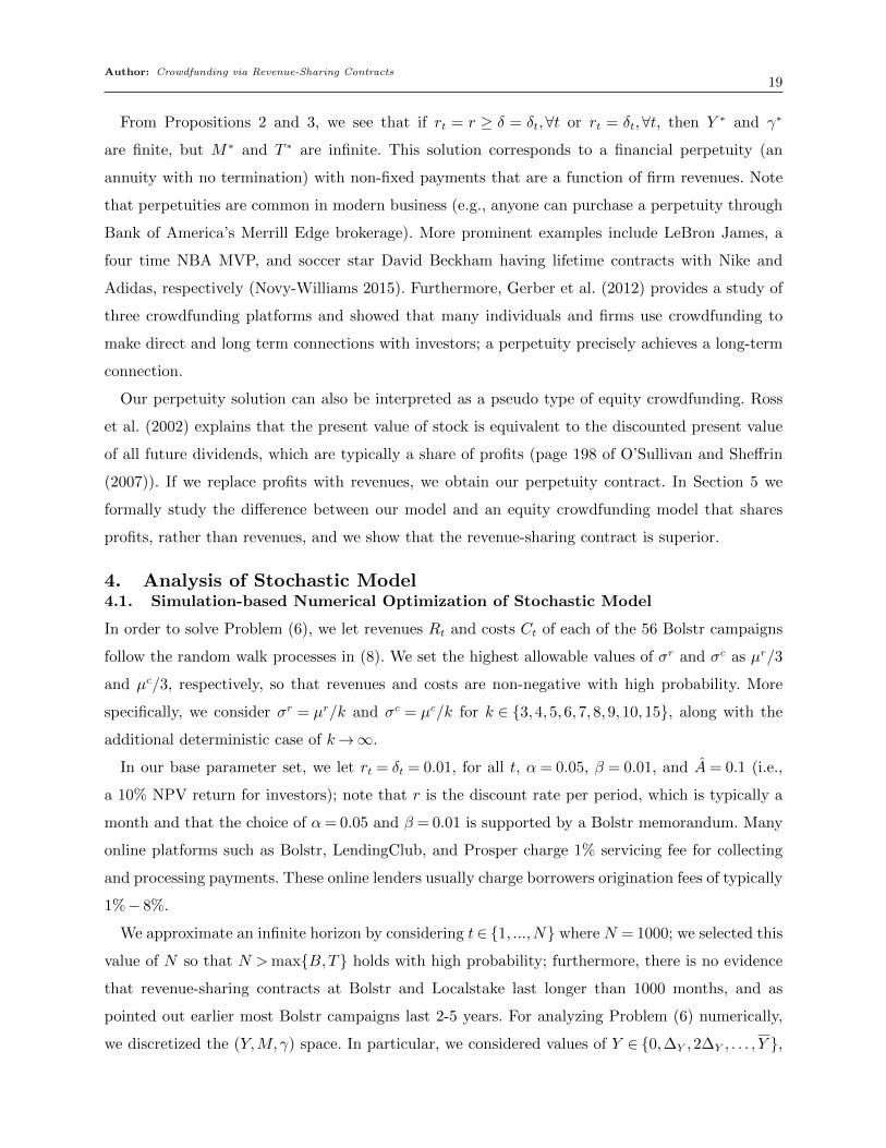
error for the stochastic problem. We denote this value of θ by θ∗ in the sequel. In the left panel
of Figure 3 we show that as cash-flow variability increases, θ∗ increases to provide a larger cash
buffer to absorb the additional variability.
The right panel of Figure 3 shows the percentage of feasible campaigns for Problem (6) that are
also feasible for Problem (11), for θ∗, and can therefore be approximated via the approximation
Problem (14). As the level of cash-flow uncertainty decreases, the approximation Problem (14)
provides an approximate solution for Problem (6) for almost all campaigns.
For evaluating the quality of the approximation, we input the approximation solutions
(Y (θ∗),M(θ∗), γ(θ∗)) into Model (6) and compare the firm’s expected NPV under this solution
with the true optimal expected NPV zF , calculated numerically. In the left panel of Figure 4, we
present the average error, over all feasible Bolstr campaigns, as a function of the standard devia-
tions σr and σc. The length of each bar above and below the average value is equal to the standard
deviation of the error over feasible campaigns. We observe that for the highest level of variability,
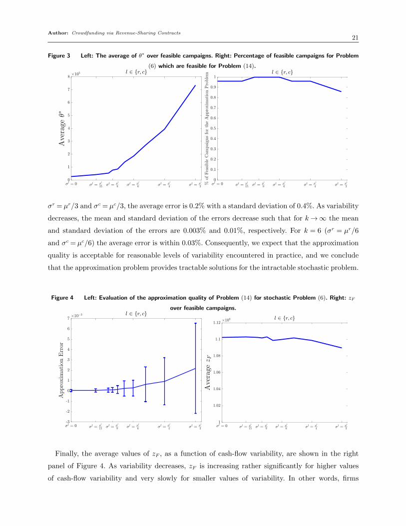
Author: Crowdfunding via Revenue-Sharing Contracts21
Figure 3 Left: The average of θ∗ over feasible campaigns. Right: Percentage of feasible campaigns for Problem
(6) which are feasible for Problem (14).
σr = µr/3 and σc = µc/3, the average error is 0.2% with a standard deviation of 0.4%. As variability
decreases, the mean and standard deviation of the errors decrease such that for k→∞ the mean
and standard deviation of the errors are 0.003% and 0.01%, respectively. For k = 6 (σr = µr/6
and σc = µc/6) the average error is within 0.03%. Consequently, we expect that the approximation
quality is acceptable for reasonable levels of variability encountered in practice, and we conclude
that the approximation problem provides tractable solutions for the intractable stochastic problem.
Figure 4 Left: Evaluation of the approximation quality of Problem (14) for stochastic Problem (6). Right: zF
over feasible campaigns.
Finally, the average values of zF , as a function of cash-flow variability, are shown in the right
panel of Figure 4. As variability decreases, zF is increasing rather significantly for higher values
of cash-flow variability and very slowly for smaller values of variability. In other words, firms

Author: Crowdfunding via Revenue-Sharing Contracts22
can increase their maximized expected NPV significantly by slightly decreasing their cash-flow
uncertainty in very uncertain environments. However, when cash-flow uncertainty is not significant,
the maximized expected NPV is slowly decreasing in the standard deviations σr and σc, and is
rather robust to their precise values.
4.3. Estimations of the T and B Distributions
In this subsection, we analyze the distributions of B, the firm’s stochastic bankruptcy time, and
T , the stochastic duration of the contract, for feasible campaigns under both the stochastic and
approximation solutions. We present results for two qualitatively different campaigns that are
feasible for all k≥ 3. One campaign, Campaign 1, has a relatively high bankruptcy probability for
k= 3 (as representative of a risky firm) and the other campaign, Campaign 2, has a zero bankruptcy
probability for k= 3 (as representative of a risk-less firm). The estimated probabilities P (B <∞)
are given in Table 1, for the optimal and approximate solutions, respectively, as a function of k.
We also evaluated the estimated probabilities P (B < T ), and they are identical to those in Table
1. We see that, as cash-flow variability decreases, the firm’s bankruptcy probability decreases for
Campaign 1 (and Campaign 2’s probability remains at zero) for both optimal and approximate
variables; furthermore, for a given k, the probabilities are mostly identical across the two sets of
variables, providing further evidence of the quality of the approximation.
Table 1 Estimated Probabilities P (B <∞).
k P (B <∞) P (B <∞) P (B <∞) P (B <∞)(σr = µr/k and σc = µc/k) for Campaign 1 for Campaign 2 for Campaign 1 for Campaign 2
for (Y ∗,M∗, γ∗) for (Y ∗,M∗, γ∗) for (Y (θ∗),M(θ∗), γ(θ∗)) for (Y (θ∗),M(θ∗), γ(θ∗))3 0.061 0 0.059 04 0.008 0 0.005 05 0.001 0 0.002 06 0.001 0 0.001 0∞ 0 0 0 0
Figure 5 shows the average of P (B <∞) over feasible Bolstr campaigns under both stochastic
and approximation solutions. The approximation solutions result in almost the same bankruptcy
probabilities as the stochastic optimal solutions, for feasible Bolstr campaigns over different levels
of cash-flow variability.
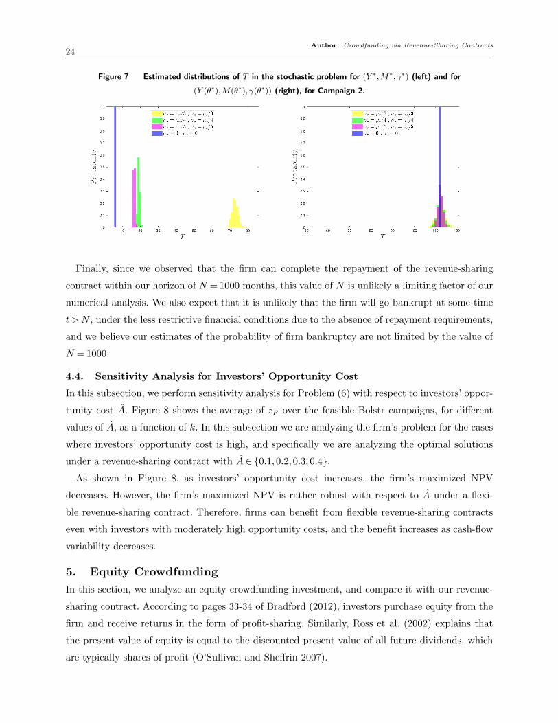
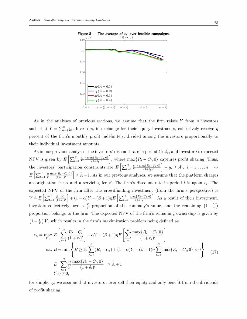
In the left plots of Figures 6 and 7, we provide the estimated distributions of T for k ∈ {3,4,5,∞}for Campaigns 1–2, respectively, for Problem (6) under the stochastic optimal solutions. Visually,
we see that the mean and standard deviation of T for the stochastic optimal solutions are decreas-
ing in k (we confirmed this numerically). In other words, as k increases, the cash-flow standard
deviations σr and σc decrease, resulting in a problem with less uncertainty, which requires less
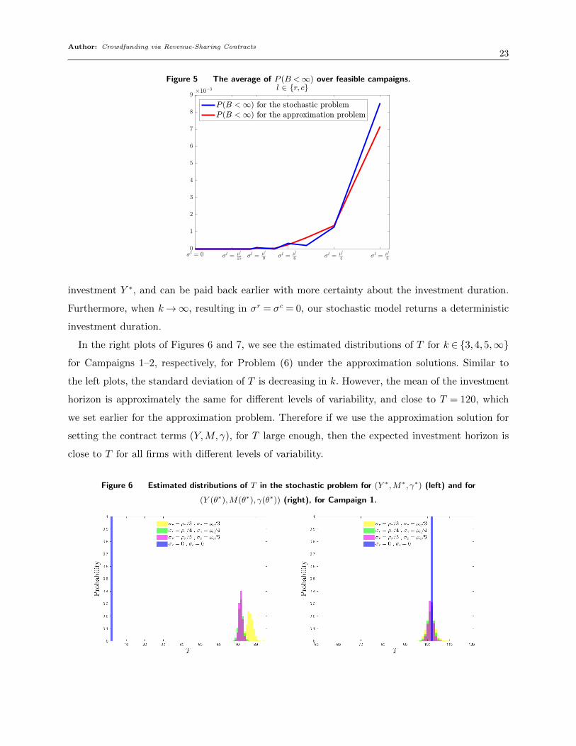
Author: Crowdfunding via Revenue-Sharing Contracts23
Figure 5 The average of P (B <∞) over feasible campaigns.
investment Y ∗, and can be paid back earlier with more certainty about the investment duration.
Furthermore, when k→∞, resulting in σr = σc = 0, our stochastic model returns a deterministic
investment duration.
In the right plots of Figures 6 and 7, we see the estimated distributions of T for k ∈ {3,4,5,∞}for Campaigns 1–2, respectively, for Problem (6) under the approximation solutions. Similar to
the left plots, the standard deviation of T is decreasing in k. However, the mean of the investment
horizon is approximately the same for different levels of variability, and close to T = 120, which
we set earlier for the approximation problem. Therefore if we use the approximation solution for
setting the contract terms (Y,M,γ), for T large enough, then the expected investment horizon is
close to T for all firms with different levels of variability.
Figure 6 Estimated distributions of T in the stochastic problem for (Y ∗,M∗, γ∗) (left) and for
(Y (θ∗),M(θ∗), γ(θ∗)) (right), for Campaign 1.
Author: Crowdfunding via Revenue-Sharing Contracts24
Figure 7 Estimated distributions of T in the stochastic problem for (Y ∗,M∗, γ∗) (left) and for
(Y (θ∗),M(θ∗), γ(θ∗)) (right), for Campaign 2.
Finally, since we observed that the firm can complete the repayment of the revenue-sharing
contract within our horizon of N = 1000 months, this value of N is unlikely a limiting factor of our
numerical analysis. We also expect that it is unlikely that the firm will go bankrupt at some time
t >N , under the less restrictive financial conditions due to the absence of repayment requirements,
and we believe our estimates of the probability of firm bankruptcy are not limited by the value of
N = 1000.
4.4. Sensitivity Analysis for Investors’ Opportunity Cost
In this subsection, we perform sensitivity analysis for Problem (6) with respect to investors’ oppor-
tunity cost A. Figure 8 shows the average of zF over the feasible Bolstr campaigns, for different
values of A, as a function of k. In this subsection we are analyzing the firm’s problem for the cases
where investors’ opportunity cost is high, and specifically we are analyzing the optimal solutions
under a revenue-sharing contract with A∈ {0.1,0.2,0.3,0.4}.As shown in Figure 8, as investors’ opportunity cost increases, the firm’s maximized NPV
decreases. However, the firm’s maximized NPV is rather robust with respect to A under a flexi-
ble revenue-sharing contract. Therefore, firms can benefit from flexible revenue-sharing contracts
even with investors with moderately high opportunity costs, and the benefit increases as cash-flow
variability decreases.
5. Equity Crowdfunding
In this section, we analyze an equity crowdfunding investment, and compare it with our revenue-
sharing contract. According to pages 33-34 of Bradford (2012), investors purchase equity from the
firm and receive returns in the form of profit-sharing. Similarly, Ross et al. (2002) explains that
the present value of equity is equal to the discounted present value of all future dividends, which
are typically shares of profit (O’Sullivan and Sheffrin 2007).
Author: Crowdfunding via Revenue-Sharing Contracts25
Figure 8 The average of zF over feasible campaigns.
As in the analyses of previous sections, we assume that the firm raises Y from n investors
such that Y =∑n
i=1 yi. Investors, in exchange for their equity investments, collectively receive η
percent of the firm’s monthly profit indefinitely, divided among the investors proportionally to
their individual investment amounts.
As in our previous analyses, the investors’ discount rate in period t is δt, and investor i’s expected
NPV is given by E[∑B
t=1yiY
ηmax{Rt−Ct,0}(1+δt)t
], where max{Rt −Ct,0} captures profit sharing. Thus,
the investors’ participation constraints are E[∑B
t=1yiY
ηmax{Rt−Ct,0}(1+δt)t
]− yi ≥ Ai, i = 1, . . . , n ⇔
E[∑B
t=1ηY
max{Rt−Ct,0}(1+δt)t
]≥ A+ 1. As in our previous analyses, we assume that the platform charges
an origination fee α and a servicing fee β. The firm’s discount rate in period t is again rt. The
expected NPV of the firm after the crowdfunding investment (from the firm’s perspective) is
V ,E[∑B
t=1Rt−Ct(1+rt)t
]+ (1−α)Y − (β + 1)ηE
[∑B
t=1max{Rt−Ct,0}
(1+rt)t
]. As a result of their investment,
investors collectively own a YV
proportion of the company’s value, and the remaining(1− Y
V
)proportion belongs to the firm. The expected NPV of the firm’s remaining ownership is given by(1− Y
V
)V , which results in the firm’s maximization problem being defined as
zE = maxY,η
E
[B∑t=1
Rt−Ct(1 + rt)t
]−αY − (β+ 1)ηE
[B∑t=1
max{Rt−Ct,0}(1 + rt)t
]
s.t. B = min
B ≥ 1 :B∑t=1
(Rt−Ct) + (1−α)Y − (β+ 1)ηB∑t=1
max{Rt−Ct,0}< 0
E
[B∑t=1
η
Y
max{Rt−Ct,0}(1 + δt)t
]≥ A+ 1
Y,η≥ 0;
(17)
for simplicity, we assume that investors never sell their equity and only benefit from the dividends
of profit sharing.
Author: Crowdfunding via Revenue-Sharing Contracts26
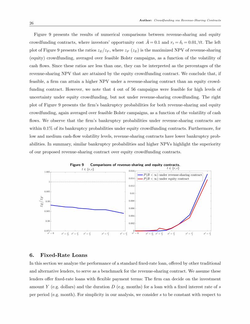
Figure 9 presents the results of numerical comparisons between revenue-sharing and equity
crowdfunding contracts, where investors’ opportunity cost A= 0.1 and rt = δt = 0.01,∀t. The left
plot of Figure 9 presents the ratios zE/zF , where zF (zE) is the maximized NPV of revenue-sharing
(equity) crowdfunding, averaged over feasible Bolstr campaigns, as a function of the volatility of
cash flows. Since these ratios are less than one, they can be interpreted as the percentages of the
revenue-sharing NPV that are attained by the equity crowdfunding contract. We conclude that, if
feasible, a firm can attain a higher NPV under a revenue-sharing contract than an equity crowd-
funding contract. However, we note that 4 out of 56 campaigns were feasible for high levels of
uncertainty under equity crowdfunding, but not under revenue-sharing crowdfunding. The right
plot of Figure 9 presents the firm’s bankruptcy probabilities for both revenue-sharing and equity
crowdfunding, again averaged over feasible Bolstr campaigns, as a function of the volatility of cash
flows. We observe that the firm’s bankruptcy probabilities under revenue-sharing contracts are
within 0.1% of its bankruptcy probabilities under equity crowdfunding contracts. Furthermore, for
low and medium cash-flow volatility levels, revenue-sharing contracts have lower bankruptcy prob-
abilities. In summary, similar bankruptcy probabilities and higher NPVs highlight the superiority
of our proposed revenue-sharing contract over equity crowdfunding contracts.
Figure 9 Comparisons of revenue-sharing and equity contracts.
6. Fixed-Rate Loans
In this section we analyze the performance of a standard fixed-rate loan, offered by other traditional
and alternative lenders, to serve as a benchmark for the revenue-sharing contract. We assume these
lenders offer fixed-rate loans with flexible payment terms: The firm can decide on the investment
amount Y (e.g. dollars) and the duration D (e.g. months) for a loan with a fixed interest rate of s
per period (e.g. month). For simplicity in our analysis, we consider s to be constant with respect to
Author: Crowdfunding via Revenue-Sharing Contracts27
D, and we show that, even for this conservative interest rate structure, revenue-sharing contracts
result in higher NPVs for firms.
The loan payment per period is a standard amortization and is equal tosY
1− (1 + s)−D(Stoft
2002). We assume the lender charges the borrower an origination fee of w percent of Y . The firm’s
maximization problem can be written as:
zL = maxY,D
E
[B∑t=1
Rt−Ct(1 + rt)t
]−E
[min{B,D}∑
t=1
sY
(1− (1 + s)−D) (1 + rt)t
]+ (1−w)Y
s.t. B = min
B ≥ 1 :B∑t=1
(Rt−Ct) + (1−w)Y −min{B,D}∑
t=1
sY
1− (1 + s)−D< 0
(bankruptcy definition)
Y,D≥ 0.(18)
Next, we solve the above problem numerically for Y and D. For this purpose, we need a
base parameter set for the monthly interest rate s. For a conservative comparison, we con-
sider w = 0. Interest rates and eligibility requirements vary across lenders. Banks usually have
more strict eligibility requirements but they offer relatively lower interest rates than some online
lenders who have less stringent eligibility requirements. We consider monthly interest rates s ∈{0.03/12,0.07/12,0.14/12,0.21/12} for the numerical analysis.
We performed the numerical analysis for D ∈ [1,120] months and Y ∈ [0,2000000]. We selected
the upper bound of D to be 120 to account for long term loans offered by the US Small Business
Administration (SBA) and banks that give more flexibility to firms. The upper bound of Y is chosen
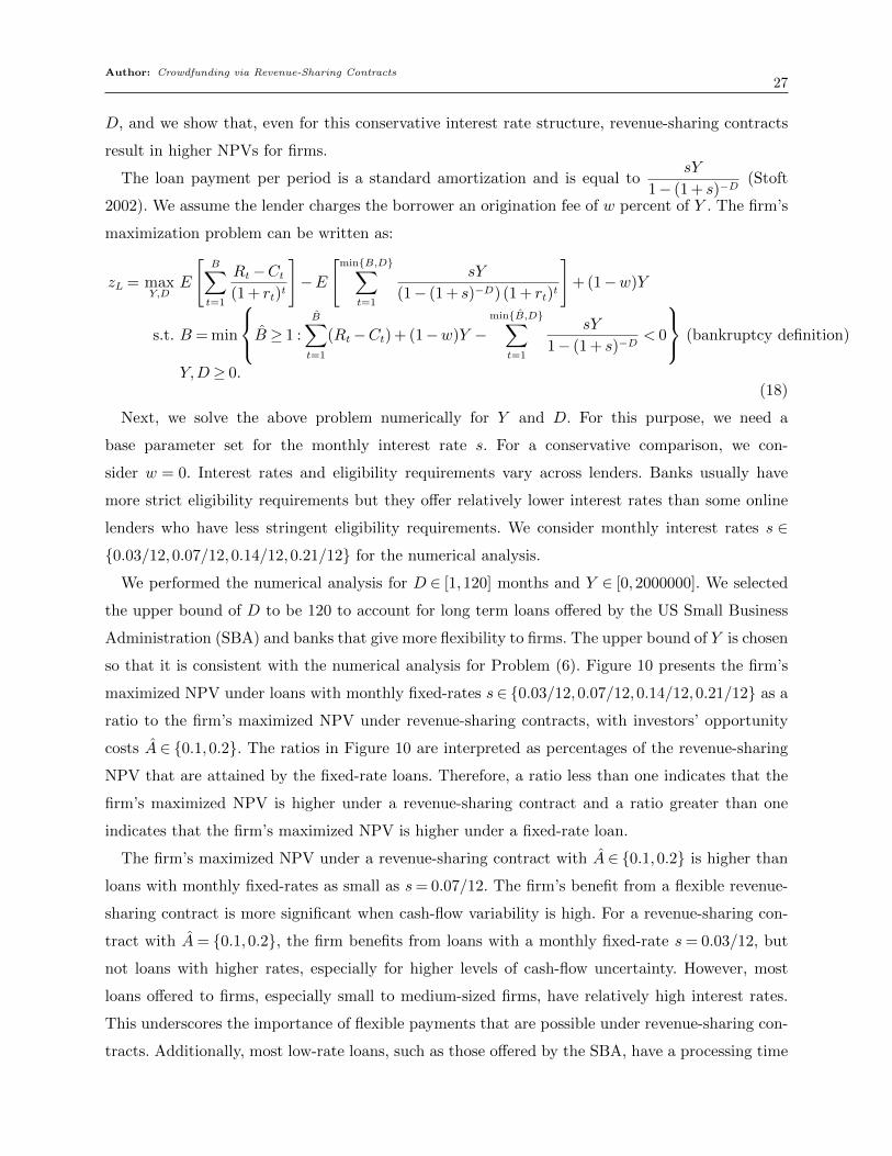
so that it is consistent with the numerical analysis for Problem (6). Figure 10 presents the firm’s
maximized NPV under loans with monthly fixed-rates s∈ {0.03/12,0.07/12,0.14/12,0.21/12} as a
ratio to the firm’s maximized NPV under revenue-sharing contracts, with investors’ opportunity
costs A ∈ {0.1,0.2}. The ratios in Figure 10 are interpreted as percentages of the revenue-sharing
NPV that are attained by the fixed-rate loans. Therefore, a ratio less than one indicates that the
firm’s maximized NPV is higher under a revenue-sharing contract and a ratio greater than one
indicates that the firm’s maximized NPV is higher under a fixed-rate loan.
The firm’s maximized NPV under a revenue-sharing contract with A ∈ {0.1,0.2} is higher than
loans with monthly fixed-rates as small as s= 0.07/12. The firm’s benefit from a flexible revenue-
sharing contract is more significant when cash-flow variability is high. For a revenue-sharing con-
tract with A= {0.1,0.2}, the firm benefits from loans with a monthly fixed-rate s= 0.03/12, but
not loans with higher rates, especially for higher levels of cash-flow uncertainty. However, most
loans offered to firms, especially small to medium-sized firms, have relatively high interest rates.
This underscores the importance of flexible payments that are possible under revenue-sharing con-
tracts. Additionally, most low-rate loans, such as those offered by the SBA, have a processing time
Author: Crowdfunding via Revenue-Sharing Contracts28
Figure 10 Comparisons of maximized NPV under revenue-sharing contracts and fixed-rate loans.
of 2–3 months. In contrast, according to marketing emails from Bolstr, firms can raise investments
under revenue-sharing contracts within hours.
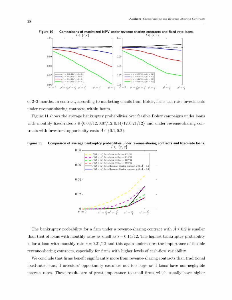
Figure 11 shows the average bankruptcy probabilities over feasible Bolstr campaigns under loans
with monthly fixed-rates s ∈ {0.03/12,0.07/12,0.14/12,0.21/12} and under revenue-sharing con-
tracts with investors’ opportunity costs A∈ {0.1,0.2}.
Figure 11 Comparison of average bankruptcy probabilities under revenue-sharing contracts and fixed-rate loans.
The bankruptcy probability for a firm under a revenue-sharing contract with A≤ 0.2 is smaller
than that of loans with monthly rates as small as s= 0.14/12. The highest bankruptcy probability
is for a loan with monthly rate s= 0.21/12 and this again underscores the importance of flexible
revenue-sharing contracts, especially for firms with higher levels of cash-flow variability.
We conclude that firms benefit significantly more from revenue-sharing contracts than traditional
fixed-rate loans, if investors’ opportunity costs are not too large or if loans have non-negligible
interest rates. These results are of great importance to small firms which usually have higher

Author: Crowdfunding via Revenue-Sharing Contracts29
levels of cash-flow uncertainty and need investment; according to a report by the SBA (U.S. Small
Business Administration 2016), 73% of small firms used some type of financing in 2015− 2016.
7. Conclusion
In this paper we analyzed an emergent model of crowdfunding in which a firm borrows capital and
then pays back investors via revenue sharing contracts. Specifically, the firm pays the investors
a percentage of its revenues monthly until a predetermined investment multiple is paid, over an
uncertain investment horizon.
This paper is the first, to our knowledge, that studies this new model of crowdfunding. This
model is facilitated by a platform (e.g., Bolstr, Localstake, or Startwise) that matches investors with
a firm needing capital. This new model helps firms in need of investment to survive and thrive with
a flexible contract whose terms depend on the firm’s performance. Indeed, when these contracts
are used optimally, we provide evidence that the likelihood of firm bankruptcy is small, even for
highly variable cash flows, due to the flexible monthly payments facilitated by the contract. If the
revenue performance of the firm goes well, then the monthly payments to investors increase, which
results in higher effective interest rates for investors. If revenue performance is poor, payments
are lowered to reduce financial stress on the firm. We use real data from 56 Bolstr campaigns to
motivate and calibrate our analytical models, and to parameterize our numerical studies.
The first part of our paper formulates a stochastic programming model of the firm’s expected
NPV maximization problem with the contract parameters as variables, for given values of the
platform’s origination and servicing fees, and investors’ opportunity costs; unfortunately, this model
is difficult to analyze. Therefore, in the second part of our paper, we formulate a deterministic
approximation that we solve analytically. In the approximation problem, we use a cash buffer for
dealing with cash-flow uncertainties. In the third part, we evaluate the quality of the approximation
solutions for the main stochastic model, over feasible Bolstr campaigns, for different levels of cash-
flow uncertainty. We see that the worst-case average error over the campaigns is approximately
0.2%. Therefore, we conclude that the approximation problem provides high quality solutions for
the intractable stochastic problem.
In the final part of our paper, we compare revenue-sharing contracts with equity crowdfunding
and fixed-rate loans. We find that, for most cases considered, revenue-sharing contracts provide
a higher NPV and a lower probability of bankruptcy than equity crowdfunding or a fixed-rate
loan. We also show that these benefits are more significant for firms with higher levels of cash-flow
uncertainty.
Acknowledgments
The second author gratefully acknowledges the support of a Neal and Jan Dempsey Faculty Fellowship.
Author: Crowdfunding via Revenue-Sharing Contracts30
References
Alois, J. D. 2016. Research: Americas alternative finance jumps to over
$36 billion in 2015. https://www.crowdfundinsider.com/2016/04/
84036-americas-alternative-finance-jumps-to-over-36-billion-in-2015. Accessed
09/21/2017.
Arrow, K. J., R. C. Lind. 1978. Uncertainty and the evaluation of public investment decisions. Uncertainty
in Economics 403–421.
Babich, V., C. S. Tang. 2016. Franchise contracting: The effects of the entrepreneur’s timing option and
debt financing. Production and Operations Management 25(4) 662–683.
Babich, V., G. Tsoukalas, S. Marinesi. 2017. Does crowdfunding benefit entrepreneurs and venture capi-
tal investors. Available at SSRN: https://ssrn.com/abstract=2971685 or http://dx.doi.org/10.
2139/ssrn.2971685.
Belleflamme, P., T. Lambert, A. Schwienbacher. 2014. Crowdfunding: Tapping the right crowd. Journal of
Business Venturing 29(5) 585–609.
Bradford, C. S. 2012. Crowdfunding and the federal securities laws. Columbia Business Law Review 1–150.
Chakraborty, S., R. Swinney. 2016. Signaling to the crowd: Private quality information and rewards-based
crowdfunding. Available at SSRN: https://ssrn.com/abstract=2885457 or http://dx.doi.org/
10.2139/ssrn.2885457.
Chase, JP Morgan, Company. 2015. Financing growth: A practical resource guide for small
businesses. https://www.jpmorganchase.com/corporate/Corporate-Responsibility/document/
icic_jpmc_apr15_rprt_web.pdf. ICIC Research Report.
Chen, Y., G. Burtch, D. Gupta. 2017. Referral timing and fundraising success in crowdfunding. Working
paper.
Cowley, S. 2016. New crowdfunding rules let the small fry swim
with sharks. https://www.nytimes.com/2016/05/15/business/dealbook/
new-crowdfunding-rules-let-the-small-fry-swim-with-sharks.html. The New York Times.
Dechow, P. M., S. P. Kothari, R. L. Watts. 1998. The relation between earnings and cash flows. Journal of
Accounting and Economics 25(2) 133–168.
Deng, S., C. Gu, G. Cai, Y. Li. 2018. Financing multiple heterogeneous suppliers in assembly systems: Buyer
finance vs. bank finance. Manufacturing & Service Operations Management Articles in Advance.
Fatehi, S., M. Wagner. 2017. Crowdfunding via revenue-sharing contracts. chapter in Supply Chain Finance,
edited by P. Kouvelis, L. Dong, and D. Turcic, Foundations and Trends in Technology, Information
and Operations Management 10(3-4) 407–424.
Friedman, M. 1955. The role of government in education. Rutgers University Press .

Author: Crowdfunding via Revenue-Sharing Contracts31
Friedman, M., S. Kuznets. 1945. Income from individual professional practice. National Bureau for Economic
Research, New York .
Gerber, E. M., J. S. Hui, P. Y. Kuo. 2012. Crowdfunding: Why people are motivated to post and fund
projects on crowdfunding platforms. Proceedings of the International Workshop on Design, Influence,
and Social Technologies: Techniques, Impacts and Ethics 2 11.
Iyer, R., A. I. Khwaja, E. F. Luttmer, K. Shue. 2015. Screening peers softly: Inferring the quality of small
borrowers. Management Science 62(6) 1554–1577.
Kac, M. 1947. Random walk and the theory of brownian motion. The American Mathematical Monthly
54(7) 369–391.
Karabell, Z. 2015. The uberization of money. https://www.wsj.com/articles/the-uberization-of-finance-
1446835102. The Wall Street Journal.
Kouvelis, P., D. Turcic, W. Zhao. 2017. Supply chain contracting in environments with volatile input prices
and frictions. Manufacturing & Service Operations Management Articles in Advance.
Kouvelis, P., W. Zhao. 2015. Supply chain contract design under financial constraints and bankruptcy costs.
Management Science 62(8) 2341–2357.
Kouvelis, P., W. Zhao. 2017. Who should finance the supply chain? impact of credit ratings on supply chain
decisions. Manufacturing & Service Operations Management Articles in Advance.
Ladine, Bret. 2001. ’70s debt program finally ending. http://yaledailynews.com/blog/2001/03/27/
70s-debt-program-finally-ending/. Accessed 9/05/2016.
Lee, H., J. Zhou, J. Wang. 2017. Trade credit financing under competition and its impact on firm performance
in supply chains. Manufacturing & Service Operations Management Articles in Advance.
Lin, M., S. Viswanathan. 2015. Home bias in online investments: An empirical study of an online crowd-
funding market. Management Science 62(5) 1393–1414.
Long, L. D., A. Ohsato. 2008. Fuzzy critical chain method for project scheduling under resource constraints
and uncertainty. International Journal of Project Management 26(6) 688–698.
Manso, G., B. Strulovici, A. Tchistyi. 2010. Performance-sensitive debt. Review of Financial Studies 23(5)
1819–1854.
Nerlove, M. 1975. Some problems in the use of income-contingent loans for the finance of higher education.
The Journal of Political Economy 83(1) 157–184.
Novy-Williams, E. 2015. Lebron james signs unprecedented lifetime con-
tract with nike. https://www.bloomberg.com/news/articles/2015-12-07/
lebron-james-signs-unprecedented-lifetime-contract-with-nike. Bloomberg.com.
Noyes, K. 2014. Why investors are pouring millions into crowdfunding. http://fortune.com/2014/04/17/
why-investors-are-pouring-millions-into-crowdfunding/.

Author: Crowdfunding via Revenue-Sharing Contracts32
O’Sullivan, A., S. M. Sheffrin. 2007. Economics: Principles in Action. Pearson Prentice Hall.
Palacios, M., A. P. Kelly. 2014. A better way to finance that college degree. https://www.wsj.com/
articles/miguel-palacios-and-andrew-kelly-a-better-way-to-finance-that-college-degree-1397428704.
Wall Street Journals.
Pratt, S. P., R. J. Grabowski, R. A. Brealey. 2014. Cost of Capital: Applications and Examples. John Wiley
& Sons.
PricewaterhouseCoopers. 2015. Peer pressure: How peer-to-peer lending platforms are transforming the con-
sumer lending industry. https://www.pwc.com/us/en/consumer-finance/publications/assets/
peer-to-peer-lending.pdf. Accessed 9/24/2017.
Purdue. 2016. https://www.purdue.edu/backaboiler/index.php. Accessed 9/19/2016.
Ross, S. A., R. A. Westerfield, J. Jaffe. 2002. Corporate Finance. McGraw-Hill Irwin. Sixth edition.
Ross, S. M. 1996. Stochastic Processes. Wiley Series in Probability and Mathematical Statistics. Second
edition.
Sigman, K. 2006. http://www.columbia.edu/~ks20/FE-Notes/4700-07-Notes-BM.pdf. IEOR 4700:
Notes on Brownian Motion.
Stoft, S. 2002. Power system economics. Journal of Energy Literature 8 94–99.
Uhrig-Homburg, M. 2005. Cash-flow shortage as an endogenous bankruptcy reason. Journal of Banking and
Finance 29(6) 1509–1534.
U.S. Securities and Exchange Commission. 2016. Regulation crowdfunding: A small entity compliance
guide for issuers[1]. https://www.sec.gov/info/smallbus/secg/rccomplianceguide-051316.htm.
Accessed 9/22/2016.
U.S. Small Business Administration. 2016. https://www.sba.gov/sites/default/files/
Finance-FAQ-2016_WEB.pdf. Accessed 09/21/2017.
Wei, Z., M. Lin. 2016. Market mechanisms in online peer-to-peer lending. Management Science 63(12)
4236–4257.
Zhang, J., P. Liu. 2012. Rational herding in microloan markets. Management Science 58(5) 892–912.

Author: Crowdfunding via Revenue-Sharing Contracts33
Appendix A: Table of Notation
Table 2 Notation
Rt stochastic revenue in period tCt stochastic cost in period trt firm’s discount rate for cash flows in period tδt investors’ discount rate for cash flows in period tyi investor i’s investment amountAi investor i’s opportunity costn number of investorsα platform’s origination fee (% of Y )β platform’s servicing fee (% of investors’ payments)
Y firm variable representing total investment amountγ firm variable representing revenue-share rateM firm variable representing guaranteed investment multipleT stochastic stopping time representing investment horizonB stochastic stopping time representing occurrence of bankruptcy
Appendix B: Proofs
Proof of Proposition 1. Using γ = MY∑Tt=1Rt
, we first substitute out γ. We then solve the problem in stages.
We first fix Y and T , and solve for the optimal M∗(Y,T ); Problem (11) simplifies to
zF (Y,T ) = maxM
(1− (β+ 1)
MY∑T
t=1Rt
)T∑t=1
Rt(1 + rt)t
+
∞∑t=T+1
Rt(1 + rt)t
−∞∑t=1
Ct(1 + rt)t
+ (1−α)Y
s.t.
(∑τ
t=1(Rt−Ct)− θ+ (1−α)Y∑min{τ,T}t=1 Rt
)(∑T
t=1Rt(β+ 1)Y
)≥M, τ ≥ 1
M ≥ (A+ 1)
∑T
t=1Rt∑T
t=1Rt
(1+δt)t
;
(19)
note that (A+1)∑Tt=1Rt∑T
t=1Rt
(1+δt)t
> 1, which implies M ≥ 1 is redundant. Problem (19), if feasible, has the solution
M∗(Y,T ) = (A+ 1)∑Tt=1Rt∑T
t=1Rt
(1+δt)t
.
We next solve for the optimal Y ∗(T ), which is the solution to the following problem
zF (T ) = maxY≥0
∞∑t=1
Rt−Ct(1 + rt)t
−(
(β+ 1)(A+ 1)
∑T
t=1Rt
(1+rt)t∑T
t=1Rt
(1+δt)t
− (1−α)
)Y
s.t.
((A+ 1)(β+ 1)
∑min{τ,T}t=1 Rt∑T
t=1Rt
(1+δt)t
− (1−α)
)Y ≤
τ∑t=1
(Rt−Ct)− θ, τ ≥ 1;
(20)
the objective is obtained by inserting the optimal M∗(Y,T ) into the objective of Problem (19); the constraints
are derived by 1) making sure the lower bound on M is smaller than the upper bound on M , making Problem
(19) feasible, and 2) inserting the optimal M∗(Y,T ) into the resulting constraints.
Using Equation (13), the constraints of Problem (20) become Zτ (T )Y ≤∑τ
t=1(Rt −Ct)− θ, for τ ≥ 1. If
τ ∈X (i.e.,∑τ
t=1(Rt−Ct)< θ), then, since Y ≥ 0, for the feasibility of Problem (20), we require Zτ (T )< 0.
If τ 6∈X (i.e.,∑τ
t=1(Rt − Ct) ≥ θ), then we consider two cases: 1) if Zτ (T ) ≤ 0, the constraint Zτ (T )Y ≤

Author: Crowdfunding via Revenue-Sharing Contracts34
∑τ
t=1(Rt − Ct)− θ is trivially true; 2) if Zτ (T ) > 0, then Y ≤∑τt=1(Rt−Ct)−θ
Zτ (T ). Thus, Problem (20) can be
written as
zF (T ) = maxY≥0
∞∑t=1
Rt−Ct(1 + rt)t
−(
(β+ 1)(A+ 1)
∑T
t=1Rt
(1+rt)t∑T
t=1Rt
(1+δt)t
− (1−α)
)Y
s.t. Y ≥maxτ∈X
{∑τ
t=1(Rt−Ct)− θZτ (T )
}Y ≤ min
τ 6∈XZτ (T )>0
{∑τ
t=1(Rt−Ct)− θZτ (T )
}.
(21)
Problem (21) is feasible if and only if Zτ (T )< 0 for all τ ∈X and
maxτ∈X
{∑τ
t=1(Rt−Ct)− θZτ (T )
}≤ min
τ 6∈XZτ (T )>0
{∑τ
t=1(Rt−Ct)− θZτ (T )
};
If (β + 1)(A+ 1)
∑Tt=1
Rt(1+rt)
t∑Tt=1
Rt(1+δt)
t
− (1− α)≥ 0, then the objective function is a decreasing function of Y and if
feasible, the solution is Y ∗(T ) = maxτ∈X
{∑τt=1(Rt−Ct)−θ
Zτ (T )
}if X 6= ∅ and Y ∗(T ) = 0 if X = ∅. Otherwise if
(β + 1)(A+ 1)
∑Tt=1
Rt(1+rt)
t∑Tt=1
Rt(1+δt)
t
− (1− α) < 0, then the objective function is an increasing function of Y and if
feasible, the solution is Y ∗(T ) = min τ 6∈XZτ (T )>0
{∑τt=1(Rt−Ct)−θ
Zτ (T )
}. �
Proof of Lemma 1. For T >max{τ : τ ∈X}, Zτ (T ) equals
(A+ 1)(β+ 1)
∑τ
t=1Rt∑T
t=1Rt
(1+δt)t
− (1−α),
which is strictly decreasing in T . The lemma’s condition (A+ 1)(β + 1)∑τt=1Rt
R∞− (1− α) < 0 implies that
there exists TX where, for T > TX , Zτ (T )< 0 for all τ ∈X. �
Proof of Lemma 2. We first show that T > τ , for all τ ∈X. For a contradiction, suppose that ∃τ0 ∈Xsuch that T ≤ τ0. The cash-flow constraint of Problem (11) for τ = τ0 is
τ0∑t=1
(Rt−Ct) + (1−α)Y − (β+ 1)γ
T∑t=1
Rt ≥ θ.
Using the contractual obligation constraint of Problem (11), γ∑T
t=1Rt =MY , this inequality implies that
MY ≤∑τ0
t=1(Rt−Ct)− θ+ (1−α)Y
(β+ 1)<︸︷︷︸
since τ0 ∈X
(1−α)
(β+ 1)Y ≤︸︷︷︸
since α,β ∈ [0,1]
Y,
which contradicts the constraint M ≥ 1. Thus, T > τ for all τ ∈X.
Noting that, for τ ∈X,∑τ
t=1(Rt −Ct)− θ < 0 and Zτ (T ) < 0, we expand the expression∑τt=1(Rt−Ct)−θ
Zτ (T )
using positive expressions:τ∑t=1
(Rt−Ct)− θ
Zτ (T )=
τ∑t=1
(Ct−Rt) + θ
(1−α)− (A+ 1)(β+ 1)
min{τ,T}∑t=1
Rt
T∑t=1
Rt(1 + δt)t
=
τ∑t=1
(Ct−Rt) + θ
(1−α)− (A+ 1)(β+ 1)
τ∑t=1
Rt
T∑t=1
Rt(1 + δt)t
, τ ∈X,
where the last equality is due to T > τ , for all τ ∈X. Consequently, as T is increased,∑τt=1(Rt−Ct)−θ
Zτ (T )strictly
decreases since Rt > 0. Since all its arguments are strictly decreasing in T , so is the maximization problem
maxτ∈X
{∑τ
t=1(Rt−Ct)− θZτ (T )
}. �

Author: Crowdfunding via Revenue-Sharing Contracts35
Proof of Lemma 3. For any τ 6∈X and T ≥ τ , the minimization argument
∑τ
t=1(Rt−Ct)− θZτ (T )
=
τ∑t=1
(Rt−Ct)− θ
(A+ 1)(β+ 1)
τ∑t=1
Rt
T∑t=1
Rt(1 + δt)t
− (1−α)
is strictly increasing in T . Note that if Zτ (T ) drops to or below zero, that argument is eliminated from
consideration; this is only possible if (A + 1)(β + 1)∑τt=1Rt
R∞< (1− α) (this condition, in Lemma 1, is for
τ ∈ X). Thus, for large enough T , each minimization argument is strictly increasing in T , and we may
conclude that minτ 6∈X
Zτ (T )>0
{∑τ
t=1(Rt−Ct)− θZτ (T )
}is also strictly increasing in T . �
Proof of Lemma 4. First we prove the lemma for rt = δt,∀t: According to Proposition 1, the objective
function of Problem (14) is simplified to
zF (T ) = maxY≥0
∞∑t=1
Rt−Ct(1 + rt)t
−(
(β+ 1)(A+ 1)− (1−α))
maxτ∈X
{∑τ
t=1(Rt−Ct)− θZτ (T )
}.
As proved in Lemma 2, maxτ∈X
{∑τt=1(Rt−Ct)−θ
Zτ (T )
}is decreasing in T and so the objective function is increasing
in T , which completes the proof for rt = δt,∀t.We next prove the lemma for rt = r≥ δ = δt,∀t for the cases where 1) (β+1)(A+1)
∑Tt=1
Rt(1+r)t∑T
t=1Rt
(1+δ)t
−(1−α)≥ 0
and 2) (β + 1)(A+ 1)
∑Tt=1
Rt(1+r)t∑T
t=1Rt
(1+δ)t
− (1− α)< 0 separately. First consider case 1: as shown in Proposition 1,
the objective function under this case is simplified to
maxY≥0
∞∑t=1
Rt−Ct(1 + r)t
−(
(β+ 1)(A+ 1)
∑T
t=1Rt
(1+r)t∑T
t=1Rt
(1+δ)t
− (1−α)
)maxτ∈X
{∑τ
t=1(Rt−Ct)− θZτ (T )
}.
The derivative of the objective function with respect to T is
dzF (T )
dT= −
((β+ 1)(A+ 1)
∑T
t=1Rt
(1+r)t∑T
t=1Rt
(1+δ)t
− (1−α)
)d(
maxτ∈X
{∑τt=1(Rt−Ct)−θ
Zτ (T )
})dT
−d
((β+ 1)(A+ 1)
∑Tt=1
Rt(1+r)t∑T
t=1Rt
(1+δ)t
− (1−α)
)dT
maxτ∈X
{∑τ
t=1(Rt−Ct)− θZτ (T )
}. (22)
If we show
∑Tt=1
Rt(1+r)t∑T
t=1Rt
(1+δ)t
is non-increasing in T , then since maxτ∈X
{∑τt=1(Rt−Ct)−θ
Zτ (T )
}is positive and decreasing
in T and (β+ 1)(A+ 1)
∑Tt=1
Rt(1+r)t∑T
t=1Rt
(1+δ)t
− (1−α)≥ 0, we conclude the objective function is increasing in T .
To show
∑Tt=1
Rt(1+r)t∑T
t=1Rt
(1+δ)t
is non-increasing in T , we calculate differences:
∑T
t=1Rt
(1+r)t∑T
t=1Rt
(1+δ)t
−∑T−1
t=1Rt
(1+r)t∑T−1t=1
Rt(1+δ)t
=
∑T
t=1Rt
(1+r)t
∑T−1t=1
Rt(1+δ)t
−∑T
t=1Rt
(1+δ)t
∑T−1t=1
Rt(1+r)t∑T
t=1Rt
(1+δ)t
∑T−1t=1
Rt(1+δ)t
=
(∑T−1t=1
Rt(1+r)t
+ RT(1+r)T
)∑T−1t=1
Rt(1+δ)t
−(∑T−1
t=1Rt
(1+δ)t+ RT
(1+δ)T
)∑T−1t=1
Rt(1+r)t∑T
t=1Rt
(1+δ)t
∑T−1t=1
Rt(1+δ)t

Author: Crowdfunding via Revenue-Sharing Contracts36
=
RT(1+r)T
∑T−1t=1
Rt(1+δ)t
− RT(1+δ)T
∑T−1t=1
Rt(1+r)t∑T
t=1Rt
(1+δ)t
∑T−1t=1
Rt(1+δ)t
=
RT(1+r)T
∑T−1t=1
Rt(1+δ)t
(1− (1+r)T
(1+δ)T
∑T−1t=1
Rt(1+r)t∑T−1
t=1Rt
(1+δ)t
)∑T
t=1Rt
(1+δ)t
∑T−1t=1
Rt(1+δ)t
=
RT(1+r)T
∑T−1t=1
Rt(1+δ)t
(1−
∑T−1t=1 Rt(1+r)
T−t∑T−1t=1 Rt(1+δ)T−t
)∑T
t=1Rt
(1+δ)t
∑T−1t=1
Rt(1+δ)t
≤ 0,
and the last inequality above holds due to r≥ δ, which completes the proof for case 1. Now consider case 2:
as shown in Proposition 1, the objective function under this case is simplified to
maxY≥0
∞∑t=1
Rt−Ct(1 + r)t
−(
(β+ 1)(A+ 1)
∑T
t=1Rt
(1+r)t∑T
t=1Rt
(1+δ)t
− (1−α)
)minτ 6∈X
Zτ (T )>0
{∑τ
t=1(Rt−Ct)− θZτ (T )
}.
The derivative of the objective function with respect to T is
dzF (T )
dT= −
((β+ 1)(A+ 1)
∑T
t=1Rt
(1+r)t∑T
t=1Rt
(1+δ)t
− (1−α)
)d(
min τ 6∈XZτ (T )>0
{∑τt=1(Rt−Ct)−θ
Zτ (T )
})dT
−d
((β+ 1)(A+ 1)
∑Tt=1
Rt(1+r)t∑T
t=1Rt
(1+δ)t
− (1−α)
)dT
minτ 6∈X
Zτ (T )>0
{∑τ
t=1(Rt−Ct)− θZτ (T )
}. (23)
As min τ 6∈XZτ (T )>0
{∑τt=1(Rt−Ct)−θ
Zτ (T )
}is positive and increasing in T and (β + 1)(A+ 1)
∑Tt=1
Rt(1+r)t∑T
t=1Rt
(1+δ)t
− (1− α) is
negative and non-increasing in T , as proved above, then we conclude the objective function is increasing in
T , which completes the proof for case 2. �
Proof of Lemma 5. If i) b < d or ii) b= d and a< c, then∑τ
t=1(Rt−Ct)− θ= (a− c)τ + (b−d) τ(τ+1)
2− θ
is unbounded from below, implying that, in either case, ∃τ0 such that τ ∈X for all τ > τ0. For any finite
T ∈N, pick a τ ∈X with τ > T ; this implies
Zτ (T ) = (A+ 1)(β+ 1)
∑T
t=1(a+ bt)∑T
t=1a+bt
(1+δt)t
− (1−α).
Since T was chosen arbitrarily, we can select it so that Zτ (T ) ≥ 0, since∑T
t=1(a + bt) is quadratic in T
and∑T
t=1a+bt
(1+δt)tgrows sub-quadratically. This proves Problem (14) is infeasible, since the first constraint is
violated, which implies that Problem (11) is also infeasible.
For iii) b = d and c ≤ a < c + θ, f(τ) can be simplified to f(τ) =(a− c)τ − θ
η(T )(aτ+b τ(τ+1)2 )−(1−α)
. Note that
limτ→∞ f(τ) = 0. Therefore minτ 6∈X
Zτ (T )>0
{f(τ)} ≤ 0 and as a result from the second constraint in Problem (14),
0≤maxτ∈X{f(τ)} ≤ min
τ 6∈XZτ (T )>0
{f(τ)} ≤ 0, we conclude Y ∗ = 0. However Y ∗ = 0 is infeasible since for b= d and
c≤ a< c+θ, the firm is cash-flow below θ in the first month: R1−C1 = (a+b)− (c+d) = a−c≤ θ. Therefore
the problem is infeasible for b= d and c≤ a< c+ θ. �
Proof of Lemma 6. We first consider the case where b > d, (b − d) ≥ (c − a) + θ, and (β + 1)(A +
1)
∑Tt=1
Rt(1+rt)
t∑Tt=1
Rt(1+δt)
t
− (1−α)≥ 0. Condition b > d implies∑τ
t=1(Rt−Ct)−θ= (a−c)τ +(b−d) τ(τ+1)
2−θ, F (τ) is

Author: Crowdfunding via Revenue-Sharing Contracts37
quadratic and convex in τ , and is minimized when τ∗ = 2(c−a)−(b−d)2(b−d) with value F (τ∗) =− (2(c−a)−(b−d))2
8(b−d) −θ <0. If τ∗ < 1 and F (1) ≥ 0, then X is empty; these conditions are equivalent to (b − d) > 2
3(c − a) and
(b−d)≥ (c−a)+θ and the latter constraint dominates (for both c≥ a and c < a, constraint (b−d)> 23(c−a)
is trivially true). Since set X is empty for b > d and (b− d) ≥ (c− a) + θ, according to Proposition 1, we
conclude Y ∗(T ) = 0 for b > d, (b− d)≥ (c− a) + θ, and (β+ 1)(A+ 1)
∑Tt=1
Rt(1+rt)
t∑Tt=1
Rt(1+δt)
t
− (1−α)≥ 0.
Next consider the case where b= d, a≥ c+θ, and (β+1)(A+1)
∑Tt=1
Rt(1+rt)
t∑Tt=1
Rt(1+δt)
t
− (1−α)≥ 0. Under conditions
b= d and a≥ c+θ,∑τ
t=1(Rt−Ct)−θ= (a−c)τ−θ is linear, and X is empty, which according to Proposition
1, we conclude Y ∗(T ) = 0 for b= d, a≥ c+ θ, and (β+ 1)(A+ 1)
∑Tt=1
Rt(1+rt)
t∑Tt=1
Rt(1+δt)
t
− (1−α)≥ 0.
Finally, consider the case where b = d, a ≥ c + θ, and (β + 1)(A + 1)
∑Tt=1
Rt(1+rt)
t∑Tt=1
Rt(1+δt)
t
− (1 − α) < 0.
According to Proposition 1, under the condition (β + 1)(A + 1)
∑Tt=1
Rt(1+rt)
t∑Tt=1
Rt(1+δt)
t
− (1 − α) < 0 we have
Y ∗(T ) = min τ 6∈XZτ (T )>0
f(τ). As shown earlier, under conditions b = d and a ≥ c + θ, set X is empty
which results in Y ∗(T ) = minτ∈N
Zτ (T )>0
f(τ). Note that Zτ (T ) = η(T )(aτ + b τ(τ+1)
2
)− (1 − α), where η(T ) =
(A+1)(β+1)∑Tt=1
Rt(1+δt)
t
> 0, is a convex function of τ ; the roots of this quadratic are−(a+ b
2)η(T )±
√(a+ b
2)2η(T )2+2bη(T )(1−α)
bη(T ).
By inspection, the smaller root is negative and the larger root is positive. This implies that
{τ ∈ N : Zτ (T ) > 0} =
{τ ∈N : τ >
−(a+ b2)η(T )+
√(a+ b
2)2η(T )2+2bη(T )(1−α)
bη(T )
}. Thus, Y ∗(T ) = min
τ∈NZτ (T )>0
f(τ) =
minτ∈N
Zτ (T )>0
(a− c)τ − θη(T )
(aτ + b τ(τ+1)
2
)− (1−α)
= limτ→∞
f(τ) = 0 for b= d, a≥ c+θ, and (β+1)(A+1)
∑Tt=1
Rt(1+rt)
t∑Tt=1
Rt(1+δt)
t
−
(1−α)< 0. �
For simplicity and tractability in the analysis, we solve the problem for θ≤ θL(T ) where θL(T ) is given by
θL(T ),2b(1−α)(b− d)/η(T ) + (cb− da)(2a+ b)−
√((cb− da)(2a+ b))
2+ 8(1−α)b(cb− da)2/η(T )
2b2.
Note that θ should be chosen such that the approximation solutions from Problem (11) are feasible for
Problem (6), and also give high quality approximations for Problem (6). In all the experiments with real
data from Bolstr, θ≤ θL(T ) suffices for high quality approximations. In extensive numerical experiments θL
is positive. In the next lemma we show θL(T ) is non-negative for b > d and b− d < c− a which indicate the
firm that has cash-flow shortages.
Lemma 16. θL(T ) is non-negative for b > d and b− d< c− a ∀ T ≥ 1.
Proof of Lemma 16. Define
∆(θ), ((1−α)(b− d)− η(T )θb)2− η(T )(cb− da) ((2(c− a)− (b− d))(1−α) + η(T )θ(2a+ b)) .
It can be verified that ∆(θ) is a quadratic convex function of θ in which θL(T ) is its smaller root and its
larger root is given by
θH(T ),2b(1−α)(b− d)/η(T ) + (cb− da)(2a+ b) +
√((cb− da)(2a+ b))
2+ 8(1−α)b(cb− da)2/η(T )
2b2.

Author: Crowdfunding via Revenue-Sharing Contracts38
As b > d at feasibility, it can be shown by inspection that θH(T )> 0. If we show ∆(θ = 0)≥ 0, then since
∆(θ) is convex with the larger root being positive, we conclude the smaller root, θL(T ), is non-negative.
Therefore we next show ∆(0) = (1 − α)2(b − d)2 − η(T )(1 − α)(cb − da)(2(c − a) − (b − d)) = (1 − α)(b −d)2(
(1−α)− η(T )(cb−da)(2(c−a)−(b−d))(b−d)2
)is non-negative. From F (τ) = 0, we know:
F (τ) = 0⇐⇒ (a− c)τ + (b− d)τ(τ + 1)/2− θ= 0⇐⇒ τ(τ + 1)/2 =θ+ (c− a)τ
(b− d).
Additionally from Zτ (T )< 0 ∀τ ∈X, we conclude Zτ (T )≤ 0 which results in
Zτ (T ) = η(T ) (aτ + bτ(τ + 1)/2)≤ (1−α)
Next we replace τ(τ + 1)/2 = θ+(c−a)τ(b−d) in the above inequality and this results in
η(T )
(aτ + b
θ+ (c− a)τ
(b− d)
)≤ (1−α)⇐⇒ η(T )
(cb− da(b− d)
τ +bθ
(b− d)
)≤ (1−α)⇐⇒
η(T )
cb− dab− d
(c− a− b−d
2
)+√(
c− a− b−d2
)2+ 2θ(b− d)
b− d +bθ
(b− d)
≤ (1−α)
Assuming the problem is feasible for θ≥ 0, we next replace θ= 0 in the above inequality:
η(T )
cb− dab− d
(c− a− b−d
2
)+√(
c− a− b−d2
)2b− d
≤ (1−α)
Since b− d < c− a, or equivalently c− a− (b− d)> 0, and b− d > 0, we can conclude c− a− (b− d)/2> 0.
From the inequality c−a− (b−d)/2> 0, we can simplify the left-hand side of the above inequality and write
it as follows:
η(T )
((cb− da)2
(c− a− b−d
2
)(b− d)2
)≤ (1−α)⇐⇒∆(0)≥ 0
and this completes the proof. �
Proof of Lemma 7. According to Proposition 1, for b > d, b − d ≥ (c − a) + θ, and (β + 1)(A +
1)
∑Tt=1
Rt(1+rt)
t∑Tt=1
Rt(1+δt)
t
− (1− α)< 0, we have Y ∗(T ) = min τ /∈XZτ (T )>0
f(τ). As shown in the proof of Proposition 6, for
b > d and b− d≥ (c− a) + θ, set X is empty. Thus, we obtain Y ∗(T ) = min τ∈NZτ (T )>0
f(τ). The derivative of
f(τ) is
df(τ)
dτ= 2
(cb− da)η(T )τ2− 2 ((1−α)(b− d)− η(T )θb) τ + (2(c− a)− (b− d))(1−α) + η(T )θ(2a+ b)
(η(T )bτ2 + (2a+ b)η(T )τ − 2(1−α))2.
We next prove the proposition for the following two cases: 1) cb− da≥ 0 and 2) cb− da< 0.
First consider case 1: cb − da ≥ 0. The numerator n(τ) of df(τ)
dτis a convex quadratic due to cb >
da. Note that, for b > d and b − d ≥ (c − a) + θ set X is empty, the numerator of f(τ) is increasing
and positive for τ ∈ [1,∞). Additionally as shown in the proof of Lemma 6, the denominator of f(τ),
Zτ (T ) = η(T )(aτ + b τ(τ+1)
2
)− (1 − α) is a convex function of τ and the roots of this quadratic are
−(a+ b2)η(T )±
√(a+ b
2)2η(T )2+2bη(T )(1−α)
bη(T ). By inspection, the smaller root is negative and the larger root is positive.
Thus for τ ∈[1,−(a+ b
2)η(T )+
√(a+ b
2)2η(T )2+2bη(T )(1−α)
bη(T )
), the denominator of f(τ) is negative and increasing
and approaches zero from below at τ ↗ −(a+ b2)η(T )+
√(a+ b
2)2η(T )2+2bη(T )(1−α)
bη(T ). Therefore as the numerator of

Author: Crowdfunding via Revenue-Sharing Contracts39
f(τ) is positive and increasing and the denominator is negative and increasing, f(τ) is strictly decreasing on
this interval, or equivalently n(τ)< 0 for τ ∈[1,−(a+ b
2)η(T )+
√(a+ b
2)2η(T )2+2bη(T )(1−α)
bη(T )
).
Alternatively, limτ→∞ n(τ) =∞. Since the numerator is convex, these observations imply that f(τ) is
unimodal on [1,∞), with a minimum at the larger root of n(τ), or
τ∗∗ =(1−α)(b− d)− η(T )θb+
√((1−α)(b− d)− η(T )θb)
2− η(T )(cb− da) ((2(c− a)− (b− d))(1−α) + η(T )θ(2a+ b))
(cb− da)η(T )
=(1−α)(b− d)− η(T )θb+
√∆(θ)
(cb− da)η(T ).
Note that τ∗∗ is real for θ ≤ θL(T ), our domain of interest. We finally prove that τ∗∗ >−(a+ b
2)η(T )+
√(a+ b
2)2η(T )2+2bη(T )(1−α)
bη(T ), which implies that τ∗∗ ∈ {τ ∈ N : Zτ (T ) > 0} and min
τ∈NZτ (T )>0
{f(τ)} =
min{f(bτ∗∗c), f(dτ∗∗e)}. If τ∗∗ ≤ −(a+ b2)η(T )+
√(a+ b
2)2η(T )2+2bη(T )(1−α)
bη(T ), then f(τ) is unimodal with a min-
imizer in
[1,−(a+ b
2)η(T )+
√(a+ b
2)2η(T )2+2bη(T )(1−α)
bη(T )
]. In particular, this implies f(τ) is increasing as τ ↗
−(a+ b2)η(T )+
√(a+ b
2)2η(T )2+2bη(T )(1−α)
bη(T ); however, this contradicts lim
τ↗−(a+ b
2)η(T )+
√(a+ b
2)2η(T )2+2bη(T )(1−α)
bη(T )
f(τ) =
−∞, since, on this domain, the denominator of f(τ), Zτ (T ), is negative and approaches zero from below,
and the numerator is positive, by the definition of X.
Next consider case 2) cb− da < 0: The numerator n(τ) of df(τ)
dτis a concave quadratic due to cb ≤ da.
Consider the smaller and larger roots of n(τ), τ∗∗ and τ∗, respectively:
τ∗∗ =−(1−α)(b− d) + η(T )θb−
√∆(θ)
(da− cb)η(T ),
and
τ∗ =−(1−α)(b− d) + η(T )θb+
√∆(θ)
(da− cb)η(T ).
As mentioned earlier, we solve the problem for θ≤ θL(T ) which guarantees the discriminant of n(τ) is non-
negative. Next we show τ∗∗ and τ∗ are negative ∀ θ ≤ θL(T ). First we show −(1 − α)(b − d) + η(T )θb <
0, ∀θ≤ θL(T ):
−(1−α)(b− d) + η(T )θb < 0, ∀θ≤ θL(T )⇐⇒−(1−α)(b− d) + η(T )θL(T )b < 0⇐⇒
−η(T )(da− cb)(2a+ b)−√
(η(T )(cb− da)(2a+ b))2
+ 8η(T )(1−α)b(cb− da)2 < 0
and the above inequality holds due to (da − cb) ≥ 0. For −(1 − α)(b − d) + η(T )θb < 0, ∀θ ≤ θL(T ), it
can be easily verified that τ∗∗ is negative. We next prove τ∗ is negative. If we rearrange the inequality
−(1− α)(b− d) + η(T )θb < 0, ∀θ ≤ θL(T ), we get θη(T )< (1− α)(b− d)/b, ∀θ ≤ θL(T ). Next we show for
θη(T ) < (1 − α)(b − d)/b, ∀θ ≤ θL(T ), the inequality −(1 − α)(a − c) + η(T )θa < 0, ∀θ ≤ θL(T ) holds by
replacing θη(T ) with its upper bound (1−α)(b− d)/b into −(1−α)(a− c) + η(T )θa < 0:
−(1−α)(a−c)+η(T )θa < 0, ∀θ≤ θL(T )⇐⇒−(1−α)(a−c)+[(1−α)(b− d)/b]a< 0⇐⇒−(1−α)(ad−cb)/b < 0

Author: Crowdfunding via Revenue-Sharing Contracts40
and the above inequality holds due to (da − cb) ≥ 0. If −(1 − α)(b − d) + η(T )θb < 0 and −(1 − α)(a −c) + η(T )θa < 0, ∀θ≤ θL(T ), then we conclude ((2(c− a)− (b− d))(1−α) + η(T )θ(2a+ b))< 0, ∀θ≤ θL(T ).
From this result, we show below that τ∗ is negative:
τ∗ ≤ 0
⇐⇒−(1−α)(b− d) + η(T )θb+√
∆(θ)≤ 0
⇐⇒−(1−α)(b− d) + η(T )θb
+
√((1−α)(b− d)− η(T )θb)
2− η(T )(cb− da) ((2(c− a)− (b− d))(1−α) + η(T )θ(2a+ b))≤ 0
⇐⇒√
((1−α)(b− d)− η(T )θb)2
+ η(T )(da− cb) ((2(c− a)− (b− d))(1−α) + η(T )θ(2a+ b))≤ (1−α)(b− d)− η(T )θb
and the above inequality holds due to (1 − α)(b − d) − η(T )θb > 0, (da − cb) ≥ 0, and
((2(c− a)− (b− d))(1−α) + η(T )θ(2a+ b)) < 0. As a result we conclude τ∗ < 0. As n(τ) is concave with
negative roots, we conclude f(τ) is strictly decreasing in [0,∞) and as a result minτ∈N
Zτ (T )>0
{f(τ)}= limτ→∞
f(τ) =
(b− d)/η(T )b. �
Proof of Lemma 8. If b > d and b−d< (c−a)+θ, then∑τ
t=1(Rt−Ct)−θ= (a−c)τ +(b−d) τ(τ+1)
2−θ,
F (τ) is a convex quadratic function of τ , and as F (0) =−θ, the smaller root is negative and the larger root
is positive and is equal to
τ ,
(c− a− b−d
2
)+√(
c− a− b−d2
)2+ 2θ(b− d)
b− d .
Note that as the discriminant is positive, the roots are real. Thus, F (τ)< 0 for 1≤ τ < τ . �
Proof of Lemma 9. Recall that Zτ (T ) = η(T )(aτ + b τ(τ+1)
2
)− (1 − α), where η(T ) = (A+1)(β+1)∑T
t=1Rt
(1+δt)t
>
0, is a convex function of τ ; the roots of this quadratic are−(a+ b
2)η(T )±
√(a+ b
2)2η(T )2+2bη(T )(1−α)
bη(T ).
By inspection, the smaller root is negative and the larger root is positive. This implies that
{τ ∈ N : Zτ (T ) < 0} =
{τ ∈N : τ <
−(a+ b2)η(T )+
√(a+ b
2)2η(T )2+2bη(T )(1−α)
bη(T )
}and {τ ∈ N : Zτ (T ) > 0} ={
τ ∈N : τ >−(a+ b
2)η(T )+
√(a+ b
2)2η(T )2+2bη(T )(1−α)
bη(T )
}. Therefore the condition Zτ (T ) < 0 for all τ ∈ X, in
which X = {τ ∈N : 0≤ τ < τ}, is equivalent to τ <−(a+ b
2)η(T )+
√(a+ b
2)2η(T )2+2bη(T )(1−α)
bη(T )or equivalently√
(c− a− (b− d)/2)2 + 2θ(b− d)<(ad−bc)+(b−d)
√(a+ b
2)2+2b(1−α)/η(T ))
b. This inequality holds if its right-hand-
side is non-negative or equivalently (ad−bc)+(b−d)√
(a+ b/2)2 + 2(1−α)b/η(T )≥ 0 . Under this condition,
the inequality can be rearranged as θ≤ θ(T ) where
θ(T ) =(b− d)2(a+ b/2)2 + 2(1−α)b(b−d)2
η(T )+ (ad− bc)2 + 2(b− d)(ad− bc)
√(a+ b/2)2 + 2(1−α)b
η(T )− b2(c− a− (b−d)
2)2
2b2(b− d).
�
According to Lemma 9, the problem is feasible for θ ≤ θ(T ). As a result we consider θ ≤min
{θ(T ), θL(T )
}, θ(T ) throughout the next set of analysis.
Proof of Lemma 10. According to Lemma 9, the first constraint in Problem (14), Zτ (T ) < 0 for all
τ ∈X, is equivalent to the conditions θ ≤ θ(T ) and (ad− bc) + (b− d)√
(a+ b/2)2 + 2(1−α)b/η(T )≥ 0. As

Author: Crowdfunding via Revenue-Sharing Contracts41
noted earlier, we solve the lemma for θ ≤ θ(T ) for Case i. Thus we prove this lemma under the conditions
(ad− bc) + (b− d)√
(a+ b/2)2 + 2(1−α)b/η(T )≥ 0, θ≤ θ(T ), b > d, b− d< (c− a) + θ, and cb > da.
The derivative of f(τ) is
df(τ)
dτ= 2
(cb− da)η(T )τ2− 2 ((1−α)(b− d)− η(T )θb) τ + (2(c− a)− (b− d))(1−α) + η(T )θ(2a+ b)
(η(T )bτ2 + (2a+ b)η(T )τ − 2(1−α))2.
The numerator n(τ) of df(τ)
dτis a convex quadratic due to cb > da. We consider the following two cases
separately:
Case 1. If n(0) = (2(c− a)− (b− d))(1−α) + η(T )θ(2a+ b)≥ 0, or equivalently θ≥ ((b−d)−2(c−a))(1−α)η(T )(2a+b)
, then
f(τ) is increasing at τ = 0. In contrast f(τ) is strictly decreasing in
[τ ,−(a+ b
2)η(T )+
√(a+ b
2)2η(T )2+2bη(T )(1−α)
bη(T )
).
The reason is as follows: for all τ ∈[τ ,−(a+ b
2)η(T )+
√(a+ b
2)2η(T )2+2bη(T )(1−α)
bη(T )
), the numerator of f(τ) is non-
negative and increasing, according to the definition of set X. As shown in Lemma 9, the denominator
of f(τ), Zτ (T ) = η(T )(aτ + b τ(τ+1)
2
)− (1 − α) is a convex function of τ and the roots of this quadratic
are−(a+ b
2)η(T )±
√(a+ b
2)2η(T )2+2bη(T )(1−α)
bη(T ). By inspection, the smaller root is negative and the larger root is
positive. Thus for τ ∈[τ ,−(a+ b
2)η(T )+
√(a+ b
2)2η(T )2+2bη(T )(1−α)
bη(T )
), the denominator of f(τ) is negative and
increasing and approaches zero from below at τ ↗ −(a+ b2)η(T )+
√(a+ b
2)2η(T )2+2bη(T )(1−α)
bη(T ). Therefore as the
numerator of f(τ) is non-negative and increasing and the denominator is negative and increasing, f(τ) is
strictly decreasing on this interval, or equivalently n(τ)< 0 for τ ∈[τ ,−(a+ b
2)η(T )+
√(a+ b
2)2η(T )2+2bη(T )(1−α)
bη(T )
).
Since n(τ) is continuous in [0, τ ], these observations imply that there is one point τ∗ in this interval where
df(τ∗)dτ
= 0. Furthermore, τ∗ must be the smaller root of the convex numerator n(τ), or
τ∗ =(1−α)(b− d)− η(T )θb−
√((1−α)(b− d)− η(T )θb)
2− η(T )(cb− da) ((2(c− a)− (b− d))(1−α) + η(T )θ(2a+ b))
(cb− da)η(T )
=(1−α)(b− d)− η(T )θb−
√∆(θ)
(cb− da)η(T ).
As shown in Lemma 16, The θL(T ) is the smaller root of the convex quadratic function ∆(θ). Therefore
for θ≤ θ(T )≤ θL(T ) which we are solving the problem for, τ∗ is real.
Consequently, df(τ)dτ
is positive for τ ∈ [0, τ∗) and negative for τ ∈ (τ∗, τ ], which implies f(τ) is unimodal on
[0, τ ], with a maximum at τ∗. Therefore, since X is a set of integers, maxτ∈X{f(τ)}= max{f(bτ∗c), f(dτ∗e)}.
Case 2. If n(0) = (2(c − a) − (b − d))(1 − α) + η(T )θ(2a + b) < 0, or equivalently θ <
((b−d)−2(c−a))(1−α)η(T )(2a+b)
, then f(τ) is strictly decreasing at τ = 0. As shown above, f(τ) is strictly decreasing on[τ ,−(a+ b
2)η(T )+
√(a+ b
2)2η(T )2+2bη(T )(1−α)
bη(T )
). Since n(τ) is a convex quadratic, these observations implies f(τ)
is strictly decreasing on [0, τ ] with a maximizer at τ = 0: maxτ∈X{f(τ)}= f(1) =
a+ b− c− d− θη(T )(a+ b)− (1−α)
. �
Proof of Lemma 11. From Lemma 9 we conclude that {τ ∈ N : τ 6∈ X, Zτ (T ) > 0} ={τ : τ >
−(a+ b2)η(T )+
√(a+ b
2)2η(T )2+2bη(T )(1−α)
bη(T )
}.
Next, building upon the proof of Lemma 10, we recall that the numerator of df(τ)
dτ, evaluated at τ = τ ,
is non-positive: n (τ)≤ 0 or equivalently f(τ) is decreasing at τ = τ . Alternatively, limτ→∞ n(τ) =∞. Since

Author: Crowdfunding via Revenue-Sharing Contracts42
the numerator is convex, these observations imply that f(τ) is unimodal on [τ ,∞), with a minimum at the
larger root of n(τ), or
τ∗∗ =(1−α)(b− d)− η(T )θb+
√((1−α)(b− d)− η(T )θb)
2− η(T )(cb− da) ((2(c− a)− (b− d))(1−α) + η(T )θ(2a+ b))
(cb− da)η(T )
=(1−α)(b− d)− η(T )θb+
√∆(θ)
(cb− da)η(T ).
Note that τ∗∗ is real for θ ≤ θ(T ) ≤ θL(T ), our domain of interest. We finally prove that
τ∗∗ >−(a+ b
2)η(T )+
√(a+ b
2)2η(T )2+2bη(T )(1−α)
bη(T ), which implies that τ∗∗ ∈ {τ ∈ N : τ 6∈ X, Zτ (T ) >
0} and minτ 6∈X
Zτ (T )>0
{f(τ)} = min{f(bτ∗∗c), f(dτ∗∗e)}. If τ∗∗ ≤ −(a+ b2)η(T )+
√(a+ b
2)2η(T )2+2bη(T )(1−α)
bη(T ), then
f(τ) is unimodal with a minimizer in
[τ ,−(a+ b
2)η(T )+
√(a+ b
2)2η(T )2+2bη(T )(1−α)
bη(T )
]. In particular, this
implies f(τ) is increasing as τ ↗ −(a+ b2)η(T )+
√(a+ b
2)2η(T )2+2bη(T )(1−α)
bη(T ); however, this contradicts
lim
τ↗−(a+ b
2)η(T )+
√(a+ b
2)2η(T )2+2bη(T )(1−α)
bη(T )
f(τ) = −∞, since, on this domain, the denominator of f(τ), Zτ (T ), is
negative and approaches zero from below, and the numerator is positive, by the definition of X. �
Proof of Lemma 12. We prove this lemma under the conditions of Lemmas 10 and 11. We first show that
the left-hand-side of maxτ∈X{f(τ)} − min
τ 6∈XZτ (T )>0
{f(τ)} ≤ 0 is increasing in θ and the inequality holds at θ = 0.
Then we conclude ∃ θ(T ) where maxτ∈X{f(τ)} ≤ min
τ 6∈XZτ (T )>0
{f(τ)} holds for θ≤ θ(T ).
First consider Case 1 in which n(0) = (2(c− a)− (b− d))(1−α) + η(T )θ(2a+ b)≥ 0, which according to
Lemmas 10–11 we have maxτ∈X{f(τ)}= max{f(bτ∗c), f(dτ∗e)} and min
τ 6∈XZτ (T )>0
{f(τ)}= min{f(bτ∗∗c), f(dτ∗∗e)}.
For ease of exposition, we assume that τ∗ and τ∗∗ are integers, so that we need to prove f(τ∗) ≤ f(τ∗∗).
Expanding the definition of f(τ), we observe
f(τ∗∗)− f(τ∗)
=(a− c)τ∗∗+ (b− d)
τ∗∗(τ∗∗+ 1)
2− θ
Zτ∗∗(T )−
(a− c)τ∗+ (b− d)τ∗(τ∗+ 1)
2− θ
Zτ∗(T )
=
((a− c)τ∗∗+ (b− d)
τ∗∗(τ∗∗+ 1)
2− θ)Zτ∗(T )−
((a− c)τ∗+ (b− d)
τ∗(τ∗+ 1)
2− θ)Zτ∗∗(T )
Zτ∗(T )Zτ∗∗(T ). (24)
From Lemma 10, we know that Zτ∗(T )< 0; similarly, from Lemma 11, we know that Zτ∗∗(T )> 0. Thus,
the denominator of Equation (24) is negative. To analyze the numerator of Equation (24), we first consider
the expression(
(a− c)t+ (b− d) t(t+1)
2− θ)Zτ (T ), which can be manipulated as follows:(
(a− c)t+ (b− d)t(t+ 1)
2− θ)Zτ (T )
=
((a− c)t+ (b− d)
t(t+ 1)
2− θ)(
η(T )
(aτ + b
τ(τ + 1)
2
)− (1−α)
)=η(T )b(b− d)
4t2τ2 +
η(T )(2a+ b)(b− d)
4t2τ − (b− d)(1−α)
2t2
−η(T )b
(2(c− a)− (b− d)
4
)tτ2− η(T )(2a+ b)
(2(c− a)− (b− d)
4
)tτ + (1−α)
(2(c− a)− (b− d)
2
)t
−θ(η(T )
(aτ + b
τ(τ + 1)
2
)− (1−α)
).

Author: Crowdfunding via Revenue-Sharing Contracts43
Since t2τ2 = τ2t2 and tτ = τt, we can write((a− c)t+ (b− d) t(t+1)
2− θ)Zτ (T )−
((a− c)τ + (b− d) τ(τ+1)
2− θ)Zt(T )
= (t− τ)((
2η(T )(bc−ad)4
)tτ − (b−d)(1−α)
2(t+ τ) + (1−α)
(2(c−a)−(b−d)
2
))+ θ (Zt(T )−Zτ (T )) . (25)
Letting t= τ∗∗ and τ = τ∗, two roots of a quadratic equation, we have that
t+τ = 2(1−α)(b− d)− η(T )θb
(cb− da)η(T ), tτ =
(2(c− a)− (b− d))(1−α) + η(T )θ(2a+ b)
(cb− da)η(T ), and (t−τ) =
2√
∆(θ)
η(T )(cb− da).
Plugging these expressions into Expression (25), along with t= τ∗∗ and τ = τ∗, we obtain
2√
∆(θ)
η(T )(cb− da)
((2(c− a)− (b− d))(1−α) + η(T )θ(a+ b/2)− (b− d)(1−α)
(b− d)(1−α)− η(T )θb
(cb− da)η(T )
)+
θ (Zτ∗∗(T )−Zτ∗(T )) .
As the denominator of Equation (24) is negative, f(τ∗∗)− f(τ∗)≥ 0 holds if the numerator of Equation (24)
is non-positive or equivalently
2√
∆(θ)
η(T )(cb− da)
((2(c− a)− (b− d))(1−α) + η(T )θ(a+ b/2)− (b− d)(1−α)
(b− d)(1−α)− η(T )θb
(cb− da)η(T )
)+
θ (Zτ∗∗(T )−Zτ∗(T ))≤ 0.
Let
g(θ) =2√
∆(θ)
η(T )(cb− da)
((2(c− a)− (b− d))(1−α) + η(T )θ(a+ b/2)− (b− d)(1−α)
(b− d)(1−α)− η(T )θb
(cb− da)η(T )
),
and
h(θ) = θη(T )(cb− da) (Zτ∗∗(T )−Zτ∗(T )) .
The above inequality is then written as g(θ) + h(θ) ≤ 0. We first show g(θ) < 0, ∀θ ≥ 0. The g(θ) can be
rearranged and written as follows:
g(θ) =2√
∆(θ)
η2(T )(cb− da)2
(−(√
∆(θ))2− η(T )θb ((1−α)(b− d)− η(T )θb)
)≤ 0.
The above inequality holds due to (1−α)(b− d)− η(T )θb≥ 0: As proved in Lemma 10, for Case 1 in which
n(0) = (2(c− a)− (b− d))(1− α) + η(T )θ(2a+ b)≥ 0, we have τ∗ ∈ [0, τ). Therefore from the definition of
τ∗, we conclude (1−α)(b− d)− η(T )θb≥ 0 must hold to have τ∗ ≥ 0. We next show that g(θ) +h(θ)< 0 at
θ= 0:
g(0) +h(0) = −2
√(((1−α)(b− d))
2− η(T )(cb− da) ((2(c− a)− (b− d))(1−α)))3
η2(T )(cb− da)2< 0.
Note that θ = 0, if feasible, belongs to this case. The reason is that from the feasibility condition b− d <c− a+ θ at θ= 0 we conclude b− d< c− a and as a result n(0)≥ 0, which is the condition of Case 1.
Recall that at feasibility we have (Zτ∗∗(T )−Zτ∗(T )) > 0 and as a result h(θ) ≥ 0. If h(θ) is decreasing
in θ, then g(θ) + h(θ) < 0, ∀θ ≥ 0. Otherwise there exists some θ(T ) ≥ 0 where g(θ) + h(θ) < 0 holds for
θ≤ θ(T )≤ θ(T ) and this completes the proof for Case 1.

Author: Crowdfunding via Revenue-Sharing Contracts44
Next we prove the left-hand-side of maxτ∈X{f(τ)} − min
τ 6∈XZτ (T )>0
{f(τ)} ≤ 0 is increasing in θ for Case 2, in
which n(0) = (2(c − a) − (b − d))(1 − α) + η(T )θ(2a + b) < 0. Then we claim, if Case 2 is feasible, there
exists some θ(T ) ≥ 0 where maxτ∈X{f(τ)} − min
τ 6∈XZτ (T )>0
{f(τ)} ≤ 0 holds for θ ≤ θ(T ) ≤ θ(T ) and this completes
the proof for Case 2. According to Lemmas 10–11, under the conditions of Case 2, we have maxτ∈X{f(τ)}=
a+ b− c− d− θη(T )(a+ b)− (1−α)
and minτ 6∈X
Zτ (T )>0
{f(τ)}= min{f(bτ∗∗c), f(dτ∗∗e)}. For ease of exposition, we assume that
τ∗∗ is integer, so maxτ∈X{f(τ)} ≤ min
τ 6∈XZτ (T )>0
{f(τ)} is equivalent to θ− ((1−α)− η(T )(a+ b))f(τ∗∗)− (a+ b) +
(c+d)≤ 0. For calculating the derivative of the left-hand-side of the above inequality with respect to θ, first
we calculate d(f(τ∗∗(θ),θ))dθ
:
d(f(τ∗∗(θ),θ))dθ
=
[((a− c) + (b− d)/2 + (b− d)τ∗∗(θ)) dτ
∗∗(θ)dθ− 1]
[η(T ) (aτ∗∗(θ) + b/2τ∗∗(θ)(τ∗∗(θ) + 1))− (1−α)]
Z2τ∗∗(θ)(T )
−
[(a− c)τ∗∗(θ) + (b− d)τ∗∗(θ)(τ∗∗(θ) + 1)/2− θ]η(T ) [a+ b/2 + bτ∗∗(θ)] dτ∗∗(θ)dθ
Z2τ∗∗(θ)(T )
=−η(T ) (aτ∗∗(θ) + bτ∗∗(θ)(τ∗∗(θ) + 1)/2)− (1−α)
Z2τ∗∗(θ)(T )
+dτ∗∗(θ)dθ
Z2τ∗∗(θ)(T )
×(η(T )τ∗∗2(θ)(cb− da)/2 + (1−α) (2(c− a)− (b− d))/2− (1−α)(b− d)τ∗∗(θ) + θη(T )(2a+ b)/2
+θη(T )bτ∗∗(θ)
).
We know τ∗∗(θ) is the root of n(τ) and therefore n(τ∗∗(θ)) = 0 or equivalently
(cb− da)η(T )τ∗∗2(θ)− 2 ((1−α)(b− d)− η(T )θb) τ∗∗(θ) + (2(c− a)− (b− d))(1−α) + η(T )θ(2a+ b) = 0,
which implies (cb − da)η(T )τ∗∗2(θ)/2 = ((1−α)(b− d)− η(T )θb) τ∗∗(θ) − (2(c − a) − (b − d))(1 − α)/2 −η(T )θ(2a + b)/2. If we replace the left-hand side of the above equation with its right-hand side into
d(f(τ∗∗(θ)(θ),θ))dθ
, the second term in d(f(τ∗∗(θ)(θ),θ))dθ
becomes zero and as a result we get
d (f(τ∗∗(θ), θ))
dθ=−η(T ) (aτ∗∗(θ) + bτ∗∗(θ)(τ∗∗(θ) + 1)/2)− (1−α)
Z2τ∗∗(θ)(T )
=− 1
Zτ∗∗(θ)(T ).
Therefore, the derivative of the left-hand side of the inequality θ− ((1−α)− η(T )(a+ b))f(τ∗∗)− (a+ b) +
(c+ d)≤ 0, with respect to θ, is
d (θ− ((1−α)− η(T )(a+ b))f(τ∗∗)− (a+ b) + (c+ d))
dθ= 1 + ((1−α)− η(T )(a+ b))
1
Zτ∗∗(θ)(T )> 0,
where the above inequality is due to Zτ∗∗(θ)(T )≥ 0, and ((1−α)− η(T )(a+ b))> 0 or equivalently Zτ=1(T )<
0, and this completes the proof for Case 2. �
Proof of Lemma 13. According to Lemma 9, the first constraint in Problem (14), Zτ (T ) < 0 for all
τ ∈X, is equivalent to the conditions θ ≤ θ(T ) and (ad− bc) + (b− d)√
(a+ b/2)2 + 2(1−α)b/η(T )≥ 0. As
noted earlier, we solve the lemma for θ ≤ θ(T ) for Case ii. Thus we prove this lemma under the conditions
(ad− bc) + (b− d)√
(a+ b/2)2 + 2(1−α)b/η(T )≥ 0, θ ≤ θ(T ), b > d, b− d < (c− a) + θ, and cb≤ da. Note
that for cb≤ da, the condition (ad− bc) + (b− d)√
(a+ b/2)2 + 2(1−α)b/η(T )≥ 0 is always satisfied.

Author: Crowdfunding via Revenue-Sharing Contracts45
The derivative of f(τ) is
df(τ)
dτ= 2
(cb− da)η(T )τ2− 2 ((1−α)(b− d)− η(T )θb) τ + (2(c− a)− (b− d))(1−α) + η(T )θ(2a+ b)
(η(T )bτ2 + (2a+ b)η(T )τ − 2(1−α))2.
The numerator n(τ) of df(τ)
dτis a concave quadratic due to cb≤ da. Consider the smaller and larger roots of
n(τ), τ∗∗ and τ∗, respectively:
τ∗∗ =−(1−α)(b− d) + η(T )θb−
√∆(θ)
(da− cb)η(T ),
and
τ∗ =−(1−α)(b− d) + η(T )θb+
√∆(θ)
(da− cb)η(T ).
As mentioned earlier, we solve the problem for θ≤ θ(T )≤ θL(T ) which guarantees the discriminant of n(τ)
is non-negative. Next we show τ∗∗ and τ∗ are negative ∀ θ≤ θL(T ). First we show −(1−α)(b−d)+η(T )θb <
0, ∀θ≤ θL(T ):
−(1−α)(b− d) + η(T )θb < 0, ∀θ≤ θL(T )⇐⇒−(1−α)(b− d) + η(T )θL(T )b < 0⇐⇒ (26)
−η(T )(da− cb)(2a+ b)−√
(η(T )(cb− da)(2a+ b))2
+ 8η(T )(1−α)b(cb− da)2 < 0 (27)
and the above inequality holds due to (da − cb) ≥ 0. For −(1 − α)(b − d) + η(T )θb < 0, ∀θ ≤ θL(T ), it
can be easily verified that τ∗∗ is negative. We next prove τ∗ is negative. If we rearrange the inequality
−(1− α)(b− d) + η(T )θb < 0, ∀θ ≤ θL(T ), we get θη(T )< (1− α)(b− d)/b, ∀θ ≤ θL(T ). Next we show for
θη(T ) < (1 − α)(b − d)/b, ∀θ ≤ θL(T ), the inequality −(1 − α)(a − c) + η(T )θa < 0, ∀θ ≤ θL(T ) holds by
replacing θη(T ) with its upper bound (1−α)(b− d)/b into −(1−α)(a− c) + η(T )θa < 0:
−(1−α)(a−c)+η(T )θa < 0, ∀θ≤ θL(T )⇐⇒−(1−α)(a−c)+[(1−α)(b− d)/b]a< 0⇐⇒−(1−α)(ad−cb)/b < 0
and the above inequality holds due to (da − cb) ≥ 0. If −(1 − α)(b − d) + η(T )θb < 0 and −(1 − α)(a −c) + η(T )θa < 0, ∀θ≤ θL(T ), then we conclude ((2(c− a)− (b− d))(1−α) + η(T )θ(2a+ b))< 0, ∀θ≤ θL(T ).
From this result, we show below that τ∗ is negative:
τ∗ ≤ 0
⇐⇒−(1−α)(b− d) + η(T )θb+√
∆(θ)≤ 0
⇐⇒−(1−α)(b− d) + η(T )θb
+
√((1−α)(b− d)− η(T )θb)
2− η(T )(cb− da) ((2(c− a)− (b− d))(1−α) + η(T )θ(2a+ b))≤ 0
⇐⇒√
((1−α)(b− d)− η(T )θb)2
+ η(T )(da− cb) ((2(c− a)− (b− d))(1−α) + η(T )θ(2a+ b))≤ (1−α)(b− d)− η(T )θb
and the above inequality holds due to (1 − α)(b − d) − η(T )θb > 0, (da − cb) ≥ 0, and
((2(c− a)− (b− d))(1−α) + η(T )θ(2a+ b)) < 0. As a result we conclude τ∗ < 0. As n(τ) is concave with
negative roots, we conclude f(τ) is strictly decreasing in [0,∞) and as a result maxτ∈X{f(τ)} = f(1) =
a+ b− c− d− θη(T )(a+ b)− (1−α)
. �
Proof of Lemma 14. Building upon the proof of Lemma 13, f(τ) is decreasing in [0,∞). These observa-
tions imply that minτ 6∈X
Zτ (T )>0
{f(τ)}= limτ→∞
f(τ) = (b− d)/η(T )b. �

Author: Crowdfunding via Revenue-Sharing Contracts46
Proof of Lemma 15. Building upon the proofs of Lemmas 13 and 14, the inequality maxτ∈X{f(τ)} ≤
minτ 6∈X
Zτ (T )>0
{f(τ)} is equivalent to θ ≤ (1−α)(b−d)+η(T )(da−cb)bη(T )
. Therefore the inequality maxτ∈X{f(τ)} ≤
minτ 6∈X
Zτ (T )>0
{f(τ)} holds for θ ≤min{θ(T ), (1−α)(b−d)+η(T )(da−cb)
bη(T )
}, b > d, b− d < (c− a) + θ, and cb ≤ da, and
this completes the proof. �


![Crowdfunding Pilot - Internetstiftelsen[crowd] Detta projekt är en pilot för att konceptutveckla, lansera och utvärdera ett nytt utlysningsinstrument för crowdfunding. Det finns](https://img.pdfslide.net/doc/110x75/6015b91a1599ab10b43d3930/crowdfunding-pilot-internetstiftelsen-crowd-detta-projekt-r-en-pilot-fr.jpg)