Cryocourse 2011 – Chichilianne

Thermodynamics: an introduction

Henri GODFRIN

CNRS Institut Néel Grenoble http://neel.cnrs.fr/

Thermodynamics is a funny subject. The first time you go through it, you don't understand it at all. The second time you go through it, you think you understand it, except for one or two small points.

The third time you go through it, you know you don't understand it, but by that time you are so used to it, it doesn't bother you any more.

(Attributed to Arnold Sommerfeld)

Definitions : Thermodynamic system : important to define what the system is :

Vessel + gas? Gas ?

Constraints : • isolated system: does not exchange energy or matter with the exterior • Closed system: does not exchange matter • Open system: exchanges matter • Adiabatic wall: does not allow exchange of heat

Thermodynamic equilibrium : does not evolve with time at the macroscopic level Out of equilibrium: when a constraint is suppressed, the system is out of equilibrium

State variables and equation of state: f (N,V,U) Extensive variables: X = Nx examples: N, V, U, M (magnetic moment)…

Intensive variables: Y(n1) = Y(n1+n2) examples: T, P, H …

State functions and exact differentials: state functions admit exact differentials

(see dE, δW, δQ later on) Transformations: the system evolves after the suppression of a constraint, or due to exchanges with the

exterior: State A State B

o Quasi-static transformation : close to the equilibrium at all stages o Isothermal: T=Cst Isobaric: P=Cst Isochoric: V=Cst Adiabatic: dQ=0

Partial derivatives :

TPV

∂∂ = variation of V associated with a variation of P, at constant T

Analytical identities: a) Let us consider 3 variables x, y, z related through f(x,y,z) = 0; then

1−

∂∂

=

∂∂

zz xy

yx

b) Two of the three variables are independent; therefore the expression of some physical

parameter can be expressed as u=u(x,y), or u=u(x,z), ...

xxxxx y

zuz

yu

zu

yu

∂∂

=

∂∂

∂∂

=

∂∂

=

∂∂

−1

c) From the relation f(x,y,z) = 0 we get: yxzxzy dz

zfdy

yfdx

xfdf ,,,0

∂∂

+

∂∂

+

∂∂

==

hence, after a simple calculation setting dx=0, dy=0 and dz=0: 1−=

∂∂

∂∂

∂∂

yxz xz

zy

yx

Thermodynamic coefficients:

Isobaric thermal expansion coefficient PT

VV

∂∂

=1α

Pressure thermal coefficient at constant volume VT

PP

∂∂

=1β

Isothermal compressibility T

T PV

V

∂∂

−=1χ

The existence of a State Equation f(P,V,T)=0 allows us to write:

1−=

∂∂

∂∂

∂∂

TVP VP

PT

TV

and then TPβχα =

Example: for the ideal gas PT T11

=== χβα

II) First Principle – Internal Energy

1) Properties of the internal energy: Microscopic view: ∑∑ ∑ ++=

iii

jijii VVkE

,, (sum of kinetic, potential and interaction energies of microscopic

particles)

The energy can be calculated by the laws of mechanics

Macroscopic view : Thermodynamics postulates the existence of a magnitude U the “internal energy”.

- U is conserved for an isolated system - U is a state variable - U is an extensive variable

2) Exchange of energy by Work

- Elementary work: gas in a cylinder with a piston

For a displacement dl, the work made on the gas by the external force F = P.S is dVPdlSPdlFWqs −===δ

The subscript mean “quasi-static”. This expression is valid for any thermodynamic system, of any shape.

- Finite transformation : for a finite quasi-static transformation between two equilibrium states A and

B, the system receives a work dVPWB

Aqs ∫−=

- If the transformation is NOT quasi-static, but if the external pressure is always well defined, one can calculate de work done by the external force : dVPW ext−=δ

- The process MUST be quasi-static to be able to define the “pressure” of the gas

- Remarks: -

• the variables P (intensive) and V (extensive) are called “conjugated” • We write Wδ and not dW to indicate that this is not a total differential: the Work

W characterizes the transformation, but it is not a state function!

3) Exchange of energy by Heat

We consider an elementary transformation between two macroscopic states. The expression QWdU δδ += defines the heat received by the system.

Heat is not a function of state.

Heat and Temperature: giving Heat to a system does not necessarily increase its Temperature (example of ice-water equilibrium at 0 C even when heat is applied) Temperature in an intensive magnitude, which plays for heat exchanges the same role as pressure for energy exchange by work.

Heat Capacity We consider a closed system containing one kind of molecules, with a volume V.

Heat capacity is defined as dTQC δ

α =

where Qδ is the heat received by the system, and dT the temperature increase. C is an extensive magnitude.

The index a indicates the kind of process of the transformation : PC or VC …

Useful formula: for a closed system with 3 variables (P,V,T) and two are independent, then

dVLdTCQ V +=δ (variables T and V), or dVhdTCQ P +=δ (variables T and P).

Isothermal transformation : dT = 0 and dPhdVLQ ==δ (latent heat)

Using these relations : TT

VPV

Lh χ−=

∂∂

= and VLTVLCC

PVP α=

∂∂

=−

4) Using the First Principle First principle of Thermodynamics: We postulated the existence of state function “internal energy”the variation of which is given by QWdU δδ +=

Therefore, QW δδ + is an exact differential.

Since dVPW −=δ and dVLdTCQ V +=δ then dVPLdTCdU V )( −+= for a simple, closed, system.

And hence V

V TUC

∂∂

=

TVUPL

∂∂

+=

Also, dVPW −=δ and dPhCPdTQ +=δ then PdVhdPdTCdU P −+= for a simple, closed, system.

We define a new State Function, the Enthalpy H: VPUH +=

dPVhdTCdH P )( ++=

And hence P

P THC

∂∂

= and

TPHVh

∂∂

+−=

If one uses variables T and V, then U is suitable; for T and P, better choose H!

5) Ideal gas:

The internal energy U does NOT depend on the volume V. It depends on T : U = U (T); and therefore H=H(T)

One can show easily that L = P and h = -V

and using PV=NRT : RCC VP =−

Ideal gas: case of adiabatic processes ( 0=Qδ ), with VP CC /=γ ,

One can show that ConstVPandConstVT ==− γγ 1

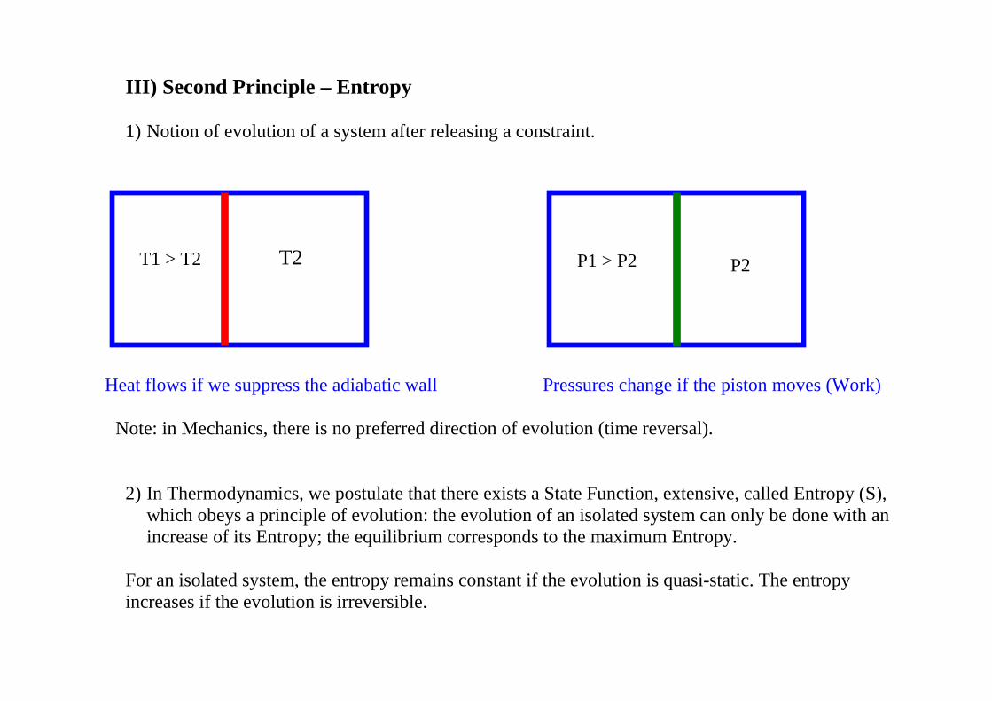
III) Second Principle – Entropy 1) Notion of evolution of a system after releasing a constraint.

Heat flows if we suppress the adiabatic wall Pressures change if the piston moves (Work) Note: in Mechanics, there is no preferred direction of evolution (time reversal).

2) In Thermodynamics, we postulate that there exists a State Function, extensive, called Entropy (S), which obeys a principle of evolution: the evolution of an isolated system can only be done with an increase of its Entropy; the equilibrium corresponds to the maximum Entropy.

For an isolated system, the entropy remains constant if the evolution is quasi-static. The entropy increases if the evolution is irreversible.

T1 > T2 T2 T1 > T2 P1 > P2 P2

3) Fundamental equations (we consider a simple, isolated system, characterized by U, V, and N)

The function ),,( NVUSS = gives all the thermodynamic information on the system. Therefore ),,( NVSUU = (“Internal Energy fundamental equation”)

dNNUdV

VUdS

SUdU

SVNSNV ,,,

∂∂

+

∂∂

+

∂∂

=

We define NVS

UT,

∂∂

= (Temperature, intensive)

and VSN

U,

∂∂

=µ (chemical potential, intensive)

and NSV

UP,

∂∂

= (pressure, intensive)

dNdVPdSTdU µ+−=

dNT

dVTPdU

TdS µ

−+=1

There exists a function, the Entropy, that can be written in terms of the extensive variables of the system.

4) Temperature and Pressure: equilibrium

The temperature T and the pressure P defined previously have the properties we expect:

The wall is initially rigid and adiabatic. The entropy is maximum. We imagine then that we allow a heat transfer from 1 to 2, with variation of volumes and internal energies:

2121 dUdUdUdVdVdV −==−== therefore

−+

−=+=

2

2

1

1

2121

11TP

TPdV

TTdUdSdSdS

Maximising S corresponds to 0=dS and this requires that

2121 PPandTT == the usual equilibrium condition !

One can show, for a membrane that allows flow of matter, that equilibrium corresponds to 21 µµ =

2 1

5) Heat and Entropy

For any transformation at constant N, we have dNdVPdSTdU µ+−= If the transformation is quasi-static, dVPW −=δ and since QWdU δδ += , then

dSTQ sq =..δ

N.B. : for an adiabatic, quasi-static transformation, ConstSanddSandQ === ,00δ (isoentropic transformation)

N.B. : For a non-quasi-static transformation, irreversibility gives rise to an additional entropy and

TQ

dS sq ..δ≥

(Clausius inequality)

N.B. : dNdVPdSTdU µ+−= (for a quasi-static transformation!) Energy heat gained work done chemical work

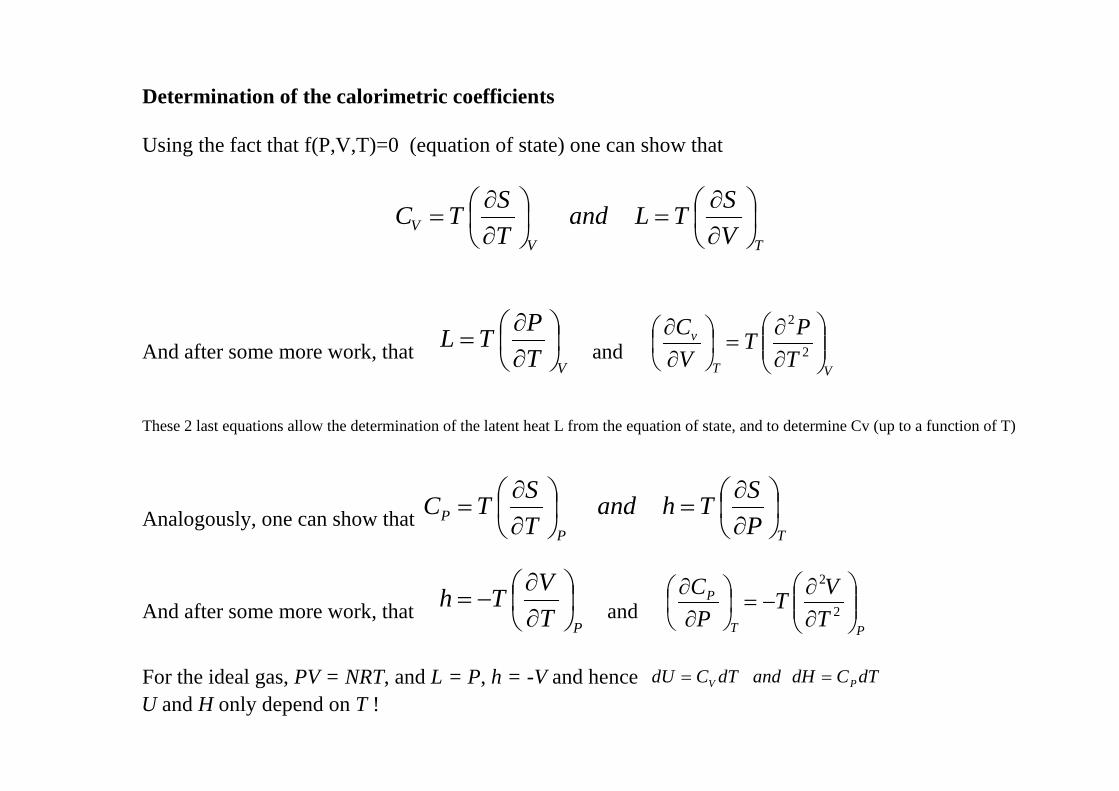
Determination of the calorimetric coefficients Using the fact that f(P,V,T)=0 (equation of state) one can show that

TVV V

STLandTSTC

∂∂

=

∂∂

=

And after some more work, that VT

PTL

∂∂

= and

VT

v

TPT

VC

∂∂

=

∂∂

2

2

These 2 last equations allow the determination of the latent heat L from the equation of state, and to determine Cv (up to a function of T)

Analogously, one can show that TP

P PSThand

TSTC

∂∂

=

∂∂

=

And after some more work, that PT

VTh

∂∂

−= and

PT

P

TVT

PC

∂∂

−=

∂∂

2

2

For the ideal gas, PV = NRT, and L = P, h = -V and hence dTCdHanddTCdU PV ==

U and H only depend on T !

III) Third Principle

Defining the temperature as NVU

ST ,

1

∂∂

= we assume that S is a continuous and derivable

function of the internal energy U. For « normal » systems, T is positive: S is a monotonous, increasing function of U.

dSTQ sq =..δ , therefore TQ

ASBS sqB

A

..)()(δ

∫=−

Can we know only variations of entropy???

Thermodynamics postulates that as T 0, S 0 (Nernst postulate)

N.B. : some expressions (ideal gas!) do not obey this Law. One can only use them for the calculation of entropy differences, in their validity range!

One can show that this implies that T 0, C 0, as well as the thermoelastic coefficients. One cannot reach the absolute Zero of temperature in a finite number of operations…

IV) Fundamental Equations – Thermodynamic Potentials 1) The fundamental equations contain all the information available on the system

U = U (S,V,N) dNdVPdSTdU µ+−=

S = S (U,V,N) dNT

dVTPdU

TdS µ

−+=1

From the first derivatives: ),,(,

NVSTSU

NV

=

∂∂

),,(,

NVSPVU

NS

=

∂∂

−

),,(,

NVSNU

VS

µ=

∂∂

From these equations, eliminating the Entropy, one obtains the Equation of State : f (P,V,N,T) = 0 We can also obtain S (T,V,N), S (T,P, N) Note that we never needed to integrate the functions: no additive (unknown constant).

From S = S (U, V, N) we get : TUS

NV

1

,

=

∂∂

TP

VS

NU

=

∂∂

, TU

SVU

µ=

∂∂

,

We have therefore T = T (U,V,N) or T = T (S,V,N) P = P (U,V,N) or P = P (S,V,N)

µ = µ (U,V,N) or µ = µ (S,V,N) These “equations of state” of the system contain also all the available information.

2) Other fundamental equations From U(S,V,N), find other fundamental equations, with other variables) Lagrange multipliers! - Free Energy (Helmholtz potential) F (sometimes called A) F = F (T,V,N)

dNdVPdTSdFSUTSTUF

NV

µ+−−=

∂∂

=−=,

- Enthalpy H H = H (S,P,N)

dNdPVdSTdHVUPVPUH

NS

µ++=

∂∂

−=+=,

- Free Enthalpy (Gibbs free energy) G G = G (T,P,N) dNdPVdTSdFSTVPUU µ++−=−+=

For a given problem, choose the potential with the adapted variables, and the corresponding fundamental equation.

One can show that U + PV – TS - µN is identically 0 (homogeneity of the function) Therefore

NG µ= and dPVdTSNd +−=µ (Gibbs – Duhem relations)

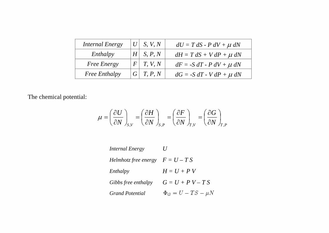
Internal Energy U S, V, N dU = T dS - P dV + µ dN Enthalpy H S, P, N dH = T dS + V dP + µ dN

Free Energy F T, V, N dF = -S dT - P dV + µ dN Free Enthalpy G T, P, N dG = -S dT - V dP + µ dN

The chemical potential:

PTVTPSVS NG

NF

NH

NU

,,,,

∂∂

=

∂∂

=

∂∂

=

∂∂

=µ

Internal Energy U

Helmhotz free energy F = U – T S

Enthalpy H = U + P V

Gibbs free enthalpy G = U + P V – T S

Grand Potential

Maxwell relations: obtained with the Schwartz condition

The Maxwell equations can be generalized for an open system : (additional relations appear, where µ plays an important role)

V) Equilibrium Conditions

Two systems are in thermal equilibrium when their temperatures are the same. Two systems are in mechanical equilibrium when their pressures are the same. Two systems are in diffusive equilibrium when their chemical potentials are the same. For a system at constant entropy and volume, ΔU = 0 at equilibrium. Minimum internal energy. For a completely isolated system, ΔS = 0 at equilibrium. Maximum Entropy. For a system at constant entropy and pressure, ΔH = 0 at equilibrium. Minimum enthalpy. N.B. the variation of H in a constant pressure transformation gives the heat transferred! For a system at constant temperature and volume, ΔF = 0 at equilibrium. Minimum Free energy. N.B. the variation of F in a constant temperature transformation gives the work done!

For a system at constant temperature and pressure, ΔG = 0 at equilibrium. Minimum Gibbs free enthalpy.

These relationships can be derived by considering the differential form of the Thermodynamic potentials

References

- Thermodynamics and an Introduction to Thermostatistics, Herbert B. Callen, John Wiley & Sons eds.

- Thermodynamics, Enrico Fermi

- Equilibrium Statistical Physics, Michael Plisschke and Birger Bergersen, Prentice Hall

(see the nice and short introduction on Thermodynamics !)

- Thermodynamique des états de la matière, Pierre Papon et Jacques Leblond, Hermann - http://en.wikipedia.org/wiki/Thermodynamics