CS 128/ES 228 - Lecture 4a 1

Spatial Data Models

CS 128/ES 228 - Lecture 4a 2

What is a spatial model?

A simplified representation of part of the real world, referenced to spatial coordinates, and created for a specific purpose

CS 128/ES 228 - Lecture 4a 3

What do you see out the window?

Naïve view: a blur of colors on my retina

Topological view: a collection of points, lines & areas in geometric relation to each other

Object-oriented view: sidewalks, buildings, trees, people …

Western NY view: a lot of snow

CS 128/ES 228 - Lecture 4a 4

Two types of features

Discrete Continuous

CS 128/ES 228 - Lecture 4a 5

What is data?

CS 128/ES 228 - Lecture 4a 6

What areare data? Observations or measurements of the real world

Three “modes” (or 3 questions to answer):

1. Spatial mode (where is it?)

2. Thematic mode (what is it?)

3. Temporal mode (when was it observed?)

CS 128/ES 228 - Lecture 4a 7

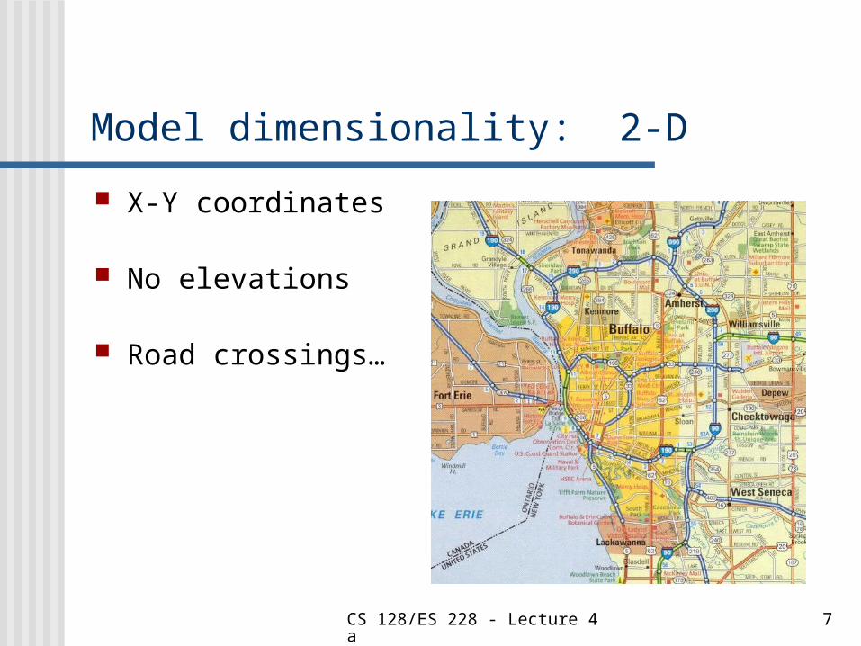
Model dimensionality: 2-D

X-Y coordinates

No elevations

Road crossings…

CS 128/ES 228 - Lecture 4a 8

Model dimensionality: 3-D

X-Y-Z coordinates

False relief

CS 128/ES 228 - Lecture 4a 9

More sophisticated 3-D models

Wire frame model“draped” withaerial photographor other surfacefeature

Thematic material can be layered on

CS 128/ES 228 - Lecture 4a 10

Model dimensionality: 4-D

X-Y-Z coordinates + temporal dimension

Fig. 7. A geographic information system representation of glacier shrinkage from 1850 to 1993 in Glacier National Park. The Blackfeet Jackson glaciers are in the center. The yellow areas reflect the current area of each glacier; other colors represent the extent of the glaciers at various times in the past. Courtesy C. Key, USGS and R. Menicke, National Park Service

CS 128/ES 228 - Lecture 4a 11

Stages of development:

1. Conceptual model: select the features of reality to be modeled and decide what entities will represent them

2. Spatial data model: select a format that will represent the model entities

3. Spatial data structure: decide how to code the entities in the model’s data files

CS 128/ES 228 - Lecture 4a 12

The modeling process

1. Conceptual model

2. Spatial datamodel

CS 128/ES 228 - Lecture 4a 13

Our local “Happy Valley”

CS 128/ES 228 - Lecture 4a 14

1. Conceptual models

Decide the model’s purpose

Select the features to be modeled

CS 128/ES 228 - Lecture 4a 15

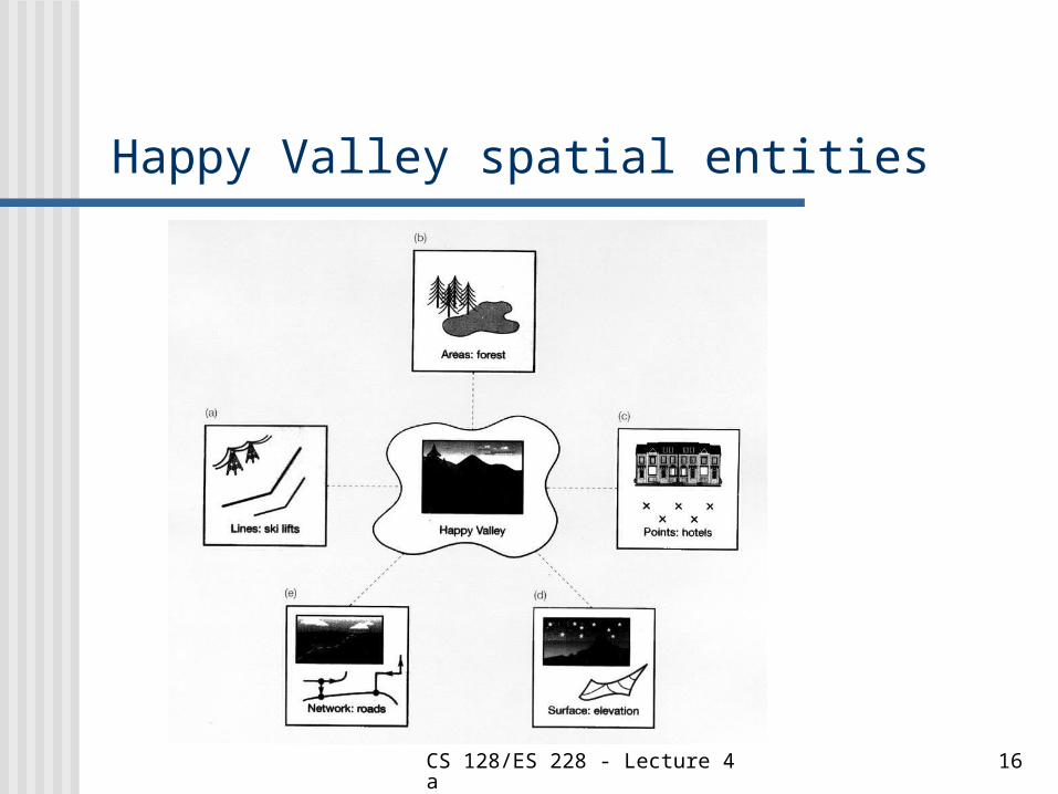
Spatial entities: 5 types

1. Points

2. Lines

3. Areas (polygons)

4. Networks

5. Surfaces

CS 128/ES 228 - Lecture 4a 16

Happy Valley spatial entities

CS 128/ES 228 - Lecture 4a 17

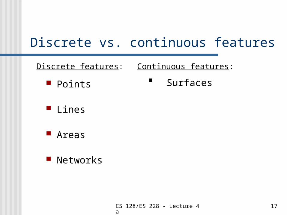
Discrete vs. continuous features

Points

Lines

Areas

Networks

Discrete features: Continuous features: Surfaces

CS 128/ES 228 - Lecture 4a 18

Networks

Line entity

Used to model features along which material, energy, or information flow

Special components: nodes, stops, turns, direction, impedance

CS 128/ES 228 - Lecture 4a 19

Impedance

CS 128/ES 228 - Lecture 4a 20

Surfaces

Continuous feature

Every location has a value, even if only interpolated from discrete samples

CS 128/ES 228 - Lecture 4a 21

Digital terrain models

CS 128/ES 228 - Lecture 4a 22

Precision agriculture

Aerial photograph Soil pH Crop yield

CS 128/ES 228 - Lecture 4a 23

Oceanography

Estimate of phytoplankton distribution in the surface ocean: global composite image of surface chlorophyll a concentration (mg m-3) estimated from SeaWiFS data (Source: NASA Goddard Space Flight Center, Maryland, USA and ORBIMAGE, Virginia, USA).