1

CS 175: Project in Artificial Intelligence

Slides 3: Regression

2

Topic 5: Regression

Slides taken from Prof. Smyth and Prof Ihler(with slight modifications)

3

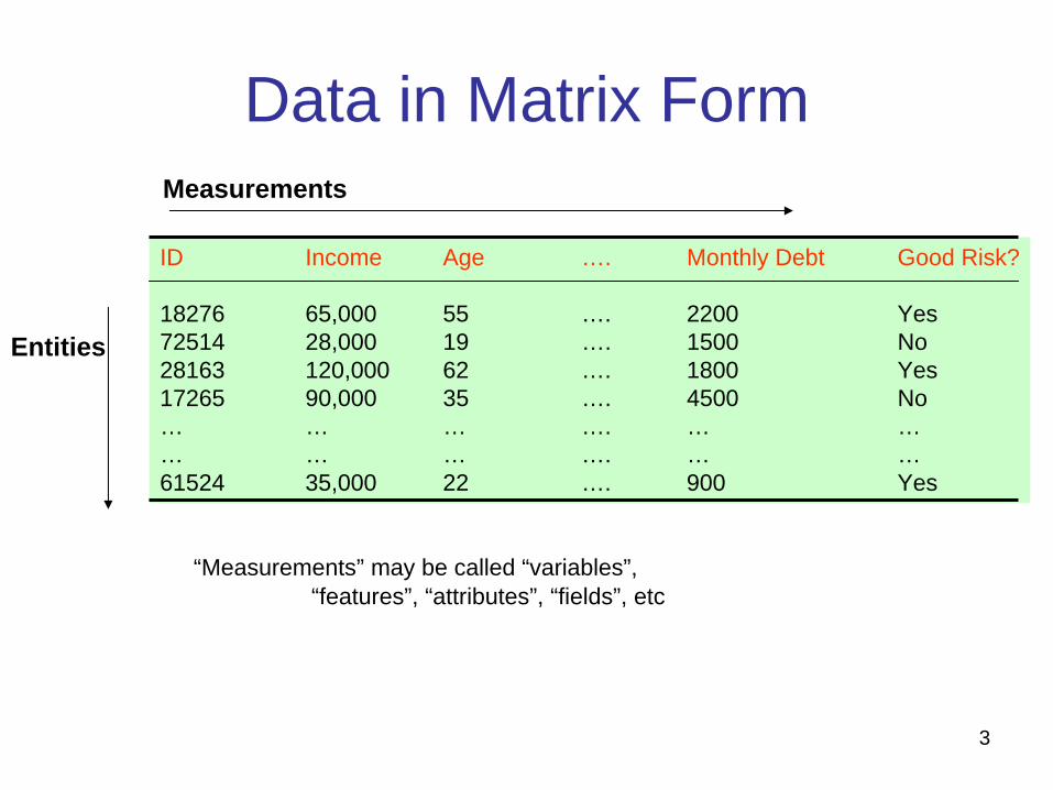
Data in Matrix Form

ID Income Age …. Monthly Debt Good Risk?

18276 65,000 55 …. 2200 Yes72514 28,000 19 …. 1500 No28163 120,000 62 …. 1800 Yes17265 90,000 35 …. 4500 No… … … …. … …… … … …. … …61524 35,000 22 …. 900 Yes

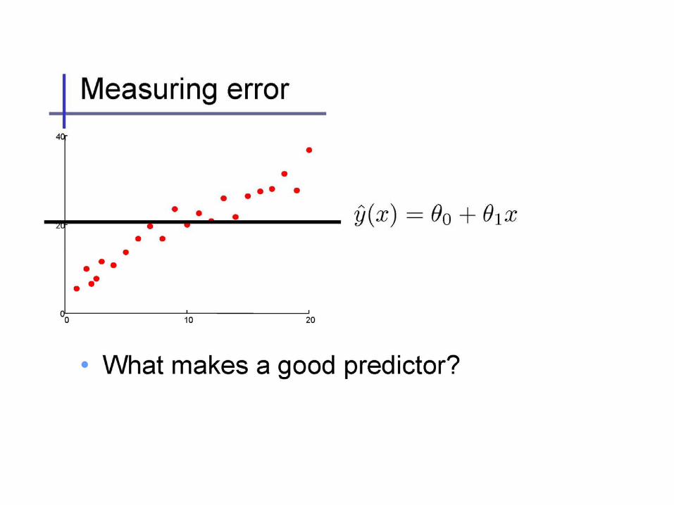
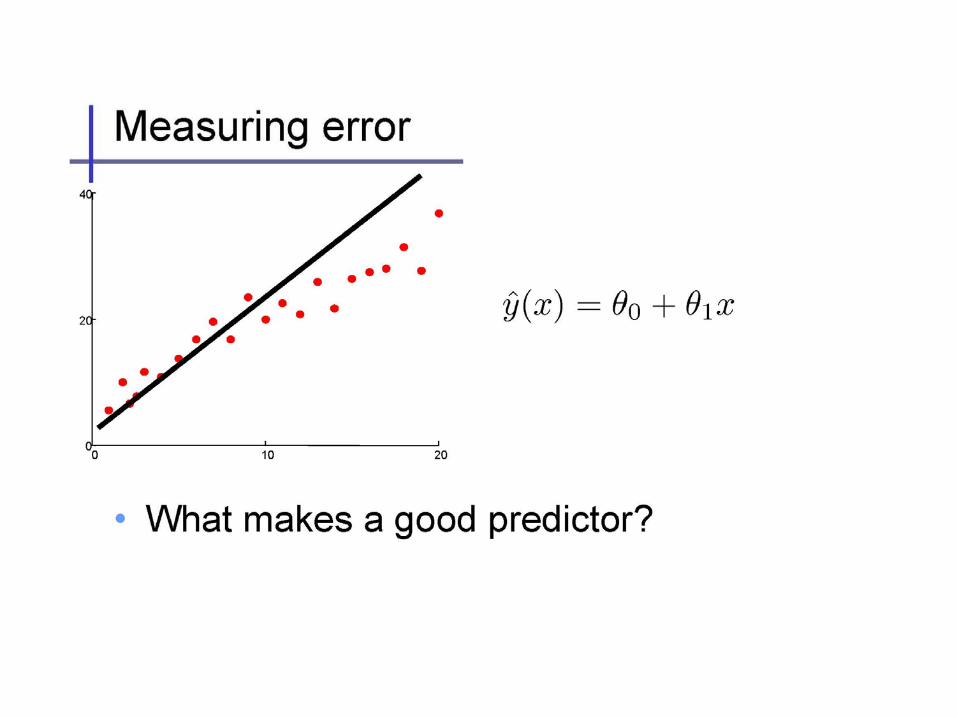
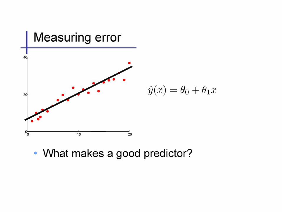
Measurements

Entities

“Measurements” may be called “variables”,“features”, “attributes”, “fields”, etc

4

5

6

7

8

9

10

11

12

13

14

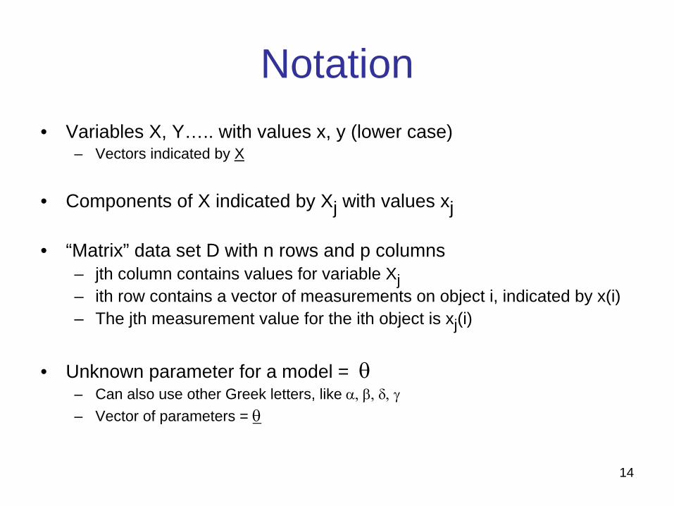
Notation• Variables X, Y….. with values x, y (lower case)

– Vectors indicated by X

• Components of X indicated by Xj with values xj

• “Matrix” data set D with n rows and p columns– jth column contains values for variable Xj– ith row contains a vector of measurements on object i, indicated by x(i)– The jth measurement value for the ith object is xj(i)

• Unknown parameter for a model = – Can also use other Greek letters, like – Vector of parameters =

15

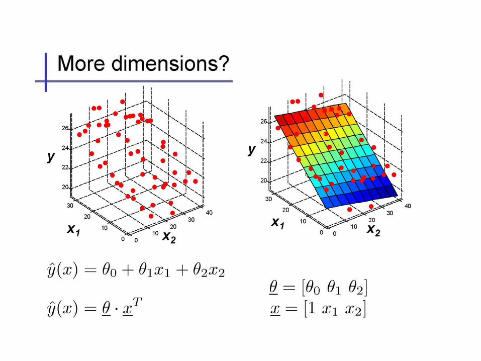
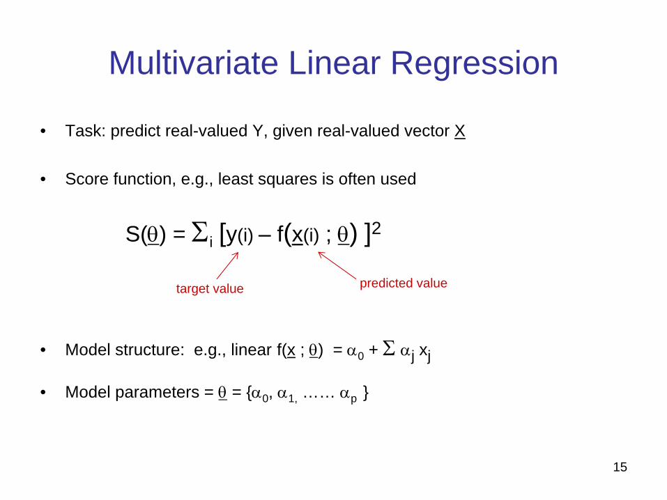
Multivariate Linear Regression

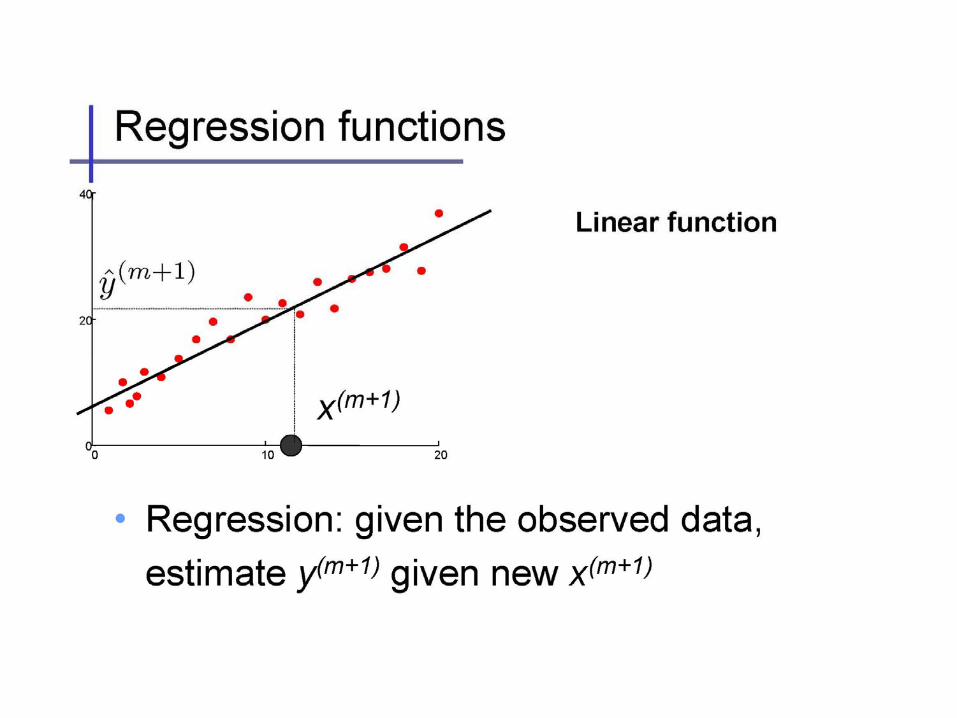
• Task: predict real-valued Y, given real-valued vector X

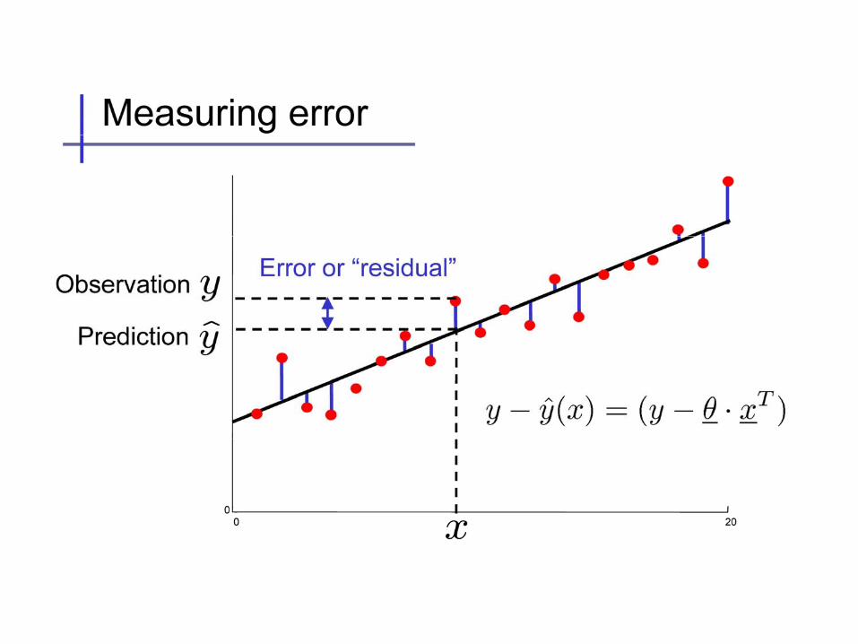
• Score function, e.g., least squares is often used

S() = i [y(i) – f(x(i) ; ) ]2

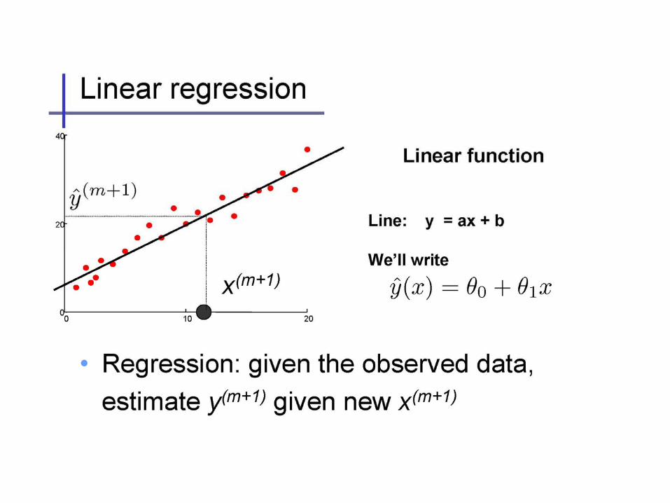
• Model structure: e.g., linear f(x ; ) = 0 +

j xj

• Model parameters =

= {0 , 1, …… p }

predicted valuetarget value

16

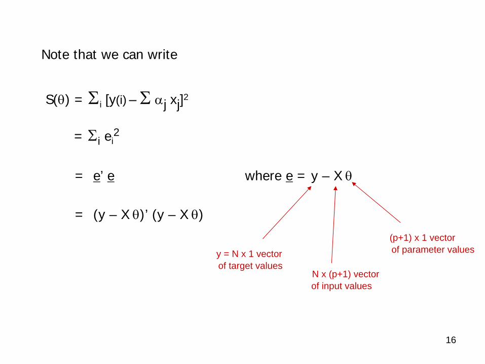
Note that we can write

S() = i [y(i) –

j xj]2

= i ei2

= e’ e where e = y – X

= (y – X )’ (y – X )

y = N x 1 vector of target values

N x (p+1) vector of input values

(p+1) x 1 vector of parameter values

17

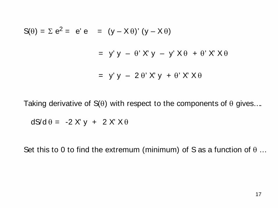
S() =

e2 = e’ e = (y – X )’ (y – X )

= y’ y – ’ X’ y – y’ X

+ ’ X’ X

= y’ y – 2 ’ X’ y + ’ X’ X

Taking derivative of S() with respect to the components of

gives….

dS/d

= -2 X’ y + 2 X’ X

Set this to 0 to find the extremum (minimum) of S as a function of …

18

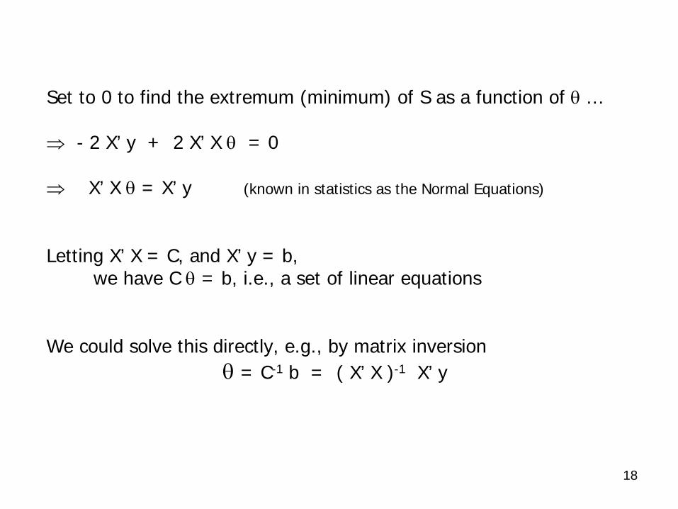
Set to 0 to find the extremum (minimum) of S as a function of …

- 2 X’ y + 2 X’ X

= 0

X’ X

= X’ y (known in statistics as the Normal Equations)

Letting X’ X = C, and X’ y = b, we have C

= b, i.e., a set of linear equations

We could solve this directly, e.g., by matrix inversion

= C-1 b = ( X’ X )-1 X’ y

19

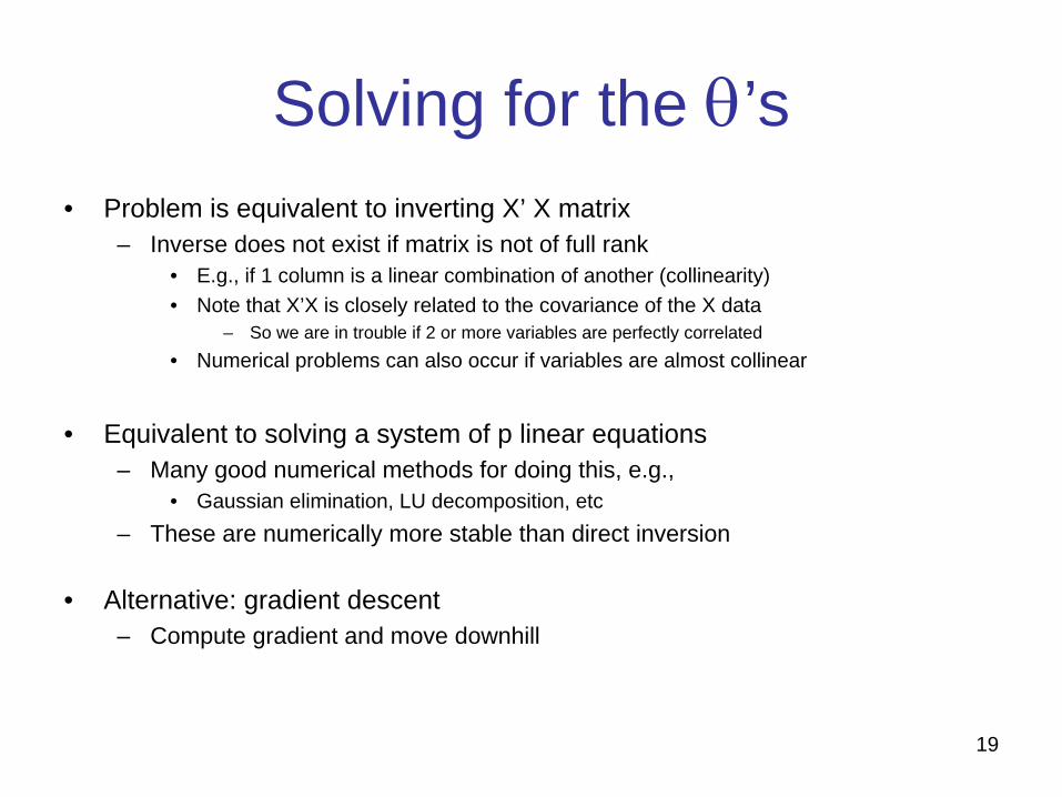
Solving for the ’s• Problem is equivalent to inverting X’ X matrix

– Inverse does not exist if matrix is not of full rank• E.g., if 1 column is a linear combination of another (collinearity)• Note that X’X is closely related to the covariance of the X data

– So we are in trouble if 2 or more variables are perfectly correlated• Numerical problems can also occur if variables are almost collinear

• Equivalent to solving a system of p linear equations– Many good numerical methods for doing this, e.g.,

• Gaussian elimination, LU decomposition, etc– These are numerically more stable than direct inversion

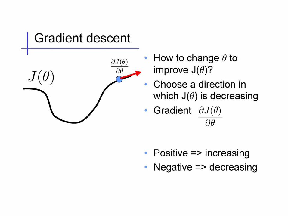
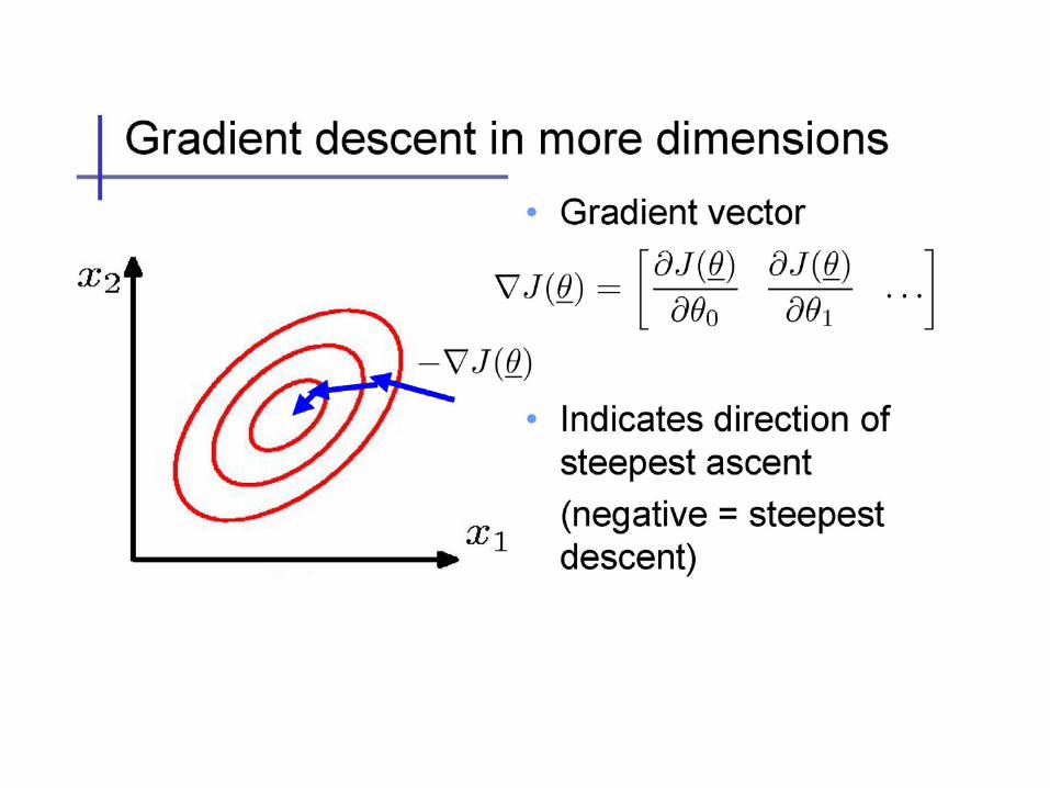
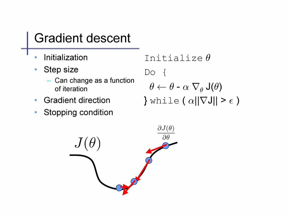
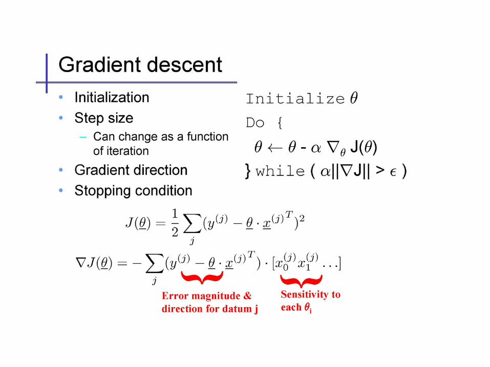
• Alternative: gradient descent– Compute gradient and move downhill

20

21

22

23

24

25

26

27

Comments on Multivariate Linear Regression

• Prediction model is a linear function of the parameters

• Score function: quadratic in predictions and parameters

Derivative of score is linear in the parameters

Leads to a linear algebra optimization problem, i.e., C

= b

• Model structure is simple….– p-1 dimensional hyperplane in p-dimensions– Linear weights => interpretability

• Often useful as a baseline model – e.g., to compare more complex models to

• Note: even if it’s the wrong model for the data (e.g., a poor fit) it can still be useful for prediction

28

Limitations of Linear Regression

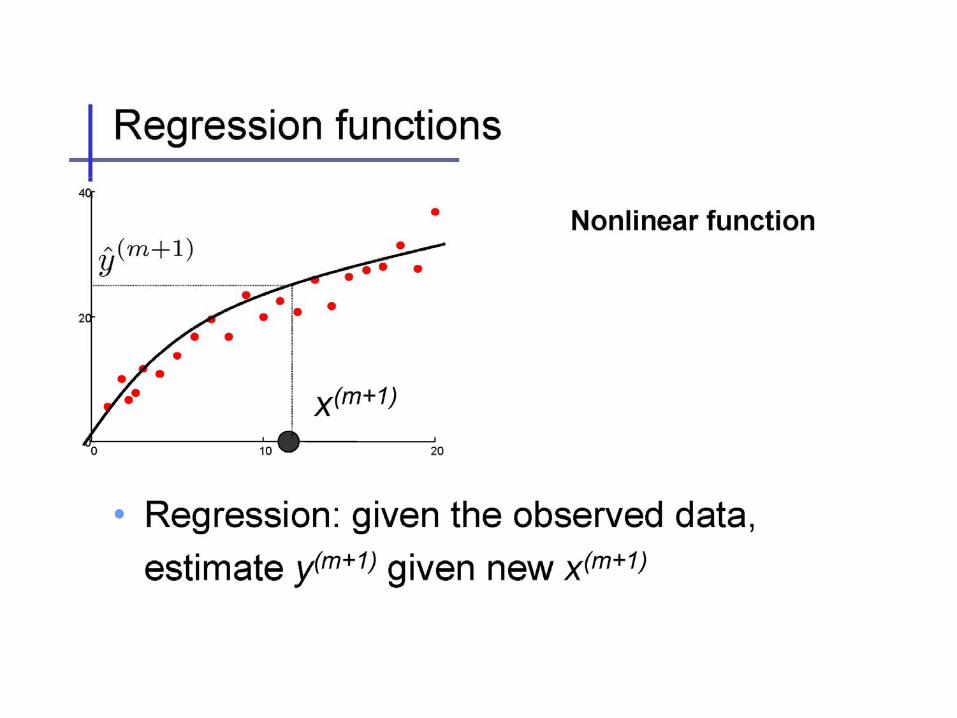
• True relationship of X and Y might be non-linear– Suggests generalizations to non-linear models

• Complexity:– O(N p2 + p3) - problematic for large p

• Correlation/Collinearity among the X variables– Can cause numerical instability (C may be ill-conditioned)– Problems in interpretability (identifiability)

• Includes all variables in the model…– But what if p=1000 and only 3 variables are actually related to Y?

29

Non-linear models, but linear in parameters

• We can add additional polynomial terms in our equations, e.g., all “2nd

order” terms f(x ; ) = 0 +

j xj +

ij xi xj

• Note that it is a non-linear functional form, but it is linear in the parameters (so still referred to as “linear regression”)– We can just treat the xi xj terms as additional fixed inputs– In fact we can add in any non-linear input functions!, e.g.

f(x ; ) = 0 +

j fj(x)

Comments:- Exact same linear algebra for optimization (same math)- Number of parameters has now exploded -> greater chance of

overfitting- Ideally would like to select only the useful quadratic terms- Can generalize this idea to higher-order interactions

30

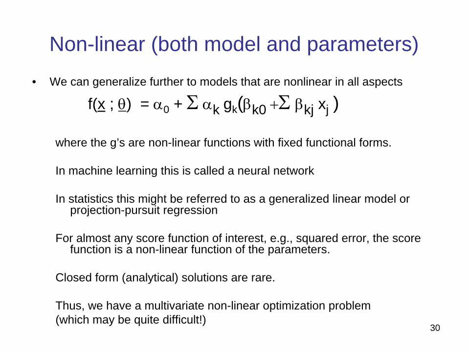
Non-linear (both model and parameters)• We can generalize further to models that are nonlinear in all aspects

f(x ; ) = 0 + k gk (k0

kj xj )

where the g’s are non-linear functions with fixed functional forms.

In machine learning this is called a neural network

In statistics this might be referred to as a generalized linear model or projection-pursuit regression

For almost any score function of interest, e.g., squared error, the score function is a non-linear function of the parameters.

Closed form (analytical) solutions are rare.

Thus, we have a multivariate non-linear optimization problem(which may be quite difficult!)

31

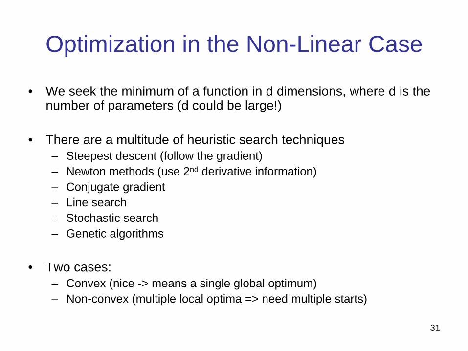
Optimization in the Non-Linear Case

• We seek the minimum of a function in d dimensions, where d is the number of parameters (d could be large!)

• There are a multitude of heuristic search techniques – Steepest descent (follow the gradient)– Newton methods (use 2nd derivative information)– Conjugate gradient– Line search– Stochastic search– Genetic algorithms

• Two cases:– Convex (nice -> means a single global optimum)– Non-convex (multiple local optima => need multiple starts)

32

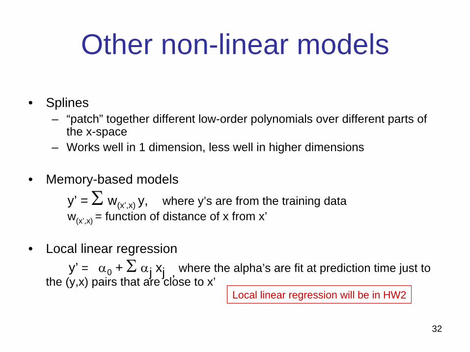
Other non-linear models

• Splines– “patch” together different low-order polynomials over different parts of

the x-space– Works well in 1 dimension, less well in higher dimensions

• Memory-based models y’ = w(x’,x) y, where y’s are from the training data w(x’,x) = function of distance of x from x’

• Local linear regression y’ = 0 +

j xj , where the alpha’s are fit at prediction time just to

the (y,x) pairs that are close to x’Local linear regression will be in HW2

33

Selecting the k best predictor variables

• Linear regression: find the best subset of k variables to put in model– This is a generic problem when p is large

(arises with all types of models, not just linear regression)

• Now we have models with different complexity..– E.g., p models with a single variable– p(p-1)/2 models with 2 variables, etc…– 2p possible models in total

• Can think of space of models as a lattice– Note that when we add or delete a variable, the optimal weights on the

other variables will change in general• k best is not the same as the best k individual variables

• Aside: what does “best” mean here? (will return to this shortly…)

34

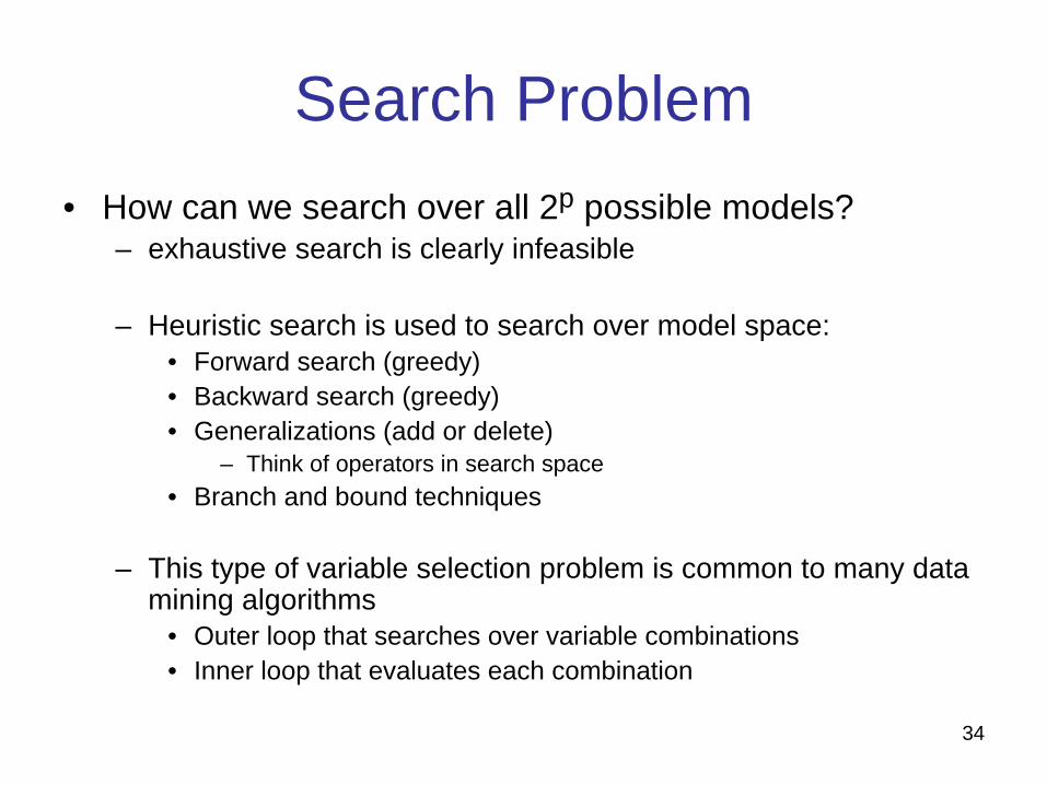
Search Problem• How can we search over all 2p possible models?

– exhaustive search is clearly infeasible

– Heuristic search is used to search over model space:• Forward search (greedy)• Backward search (greedy)• Generalizations (add or delete)

– Think of operators in search space• Branch and bound techniques

– This type of variable selection problem is common to many data mining algorithms

• Outer loop that searches over variable combinations• Inner loop that evaluates each combination

35

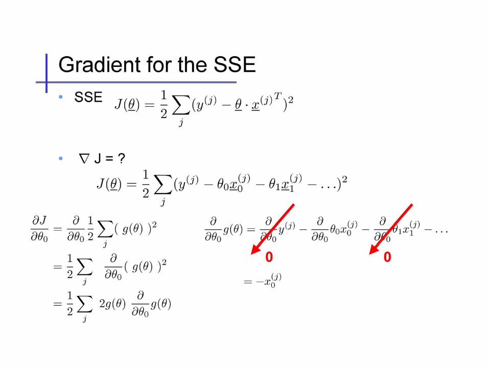
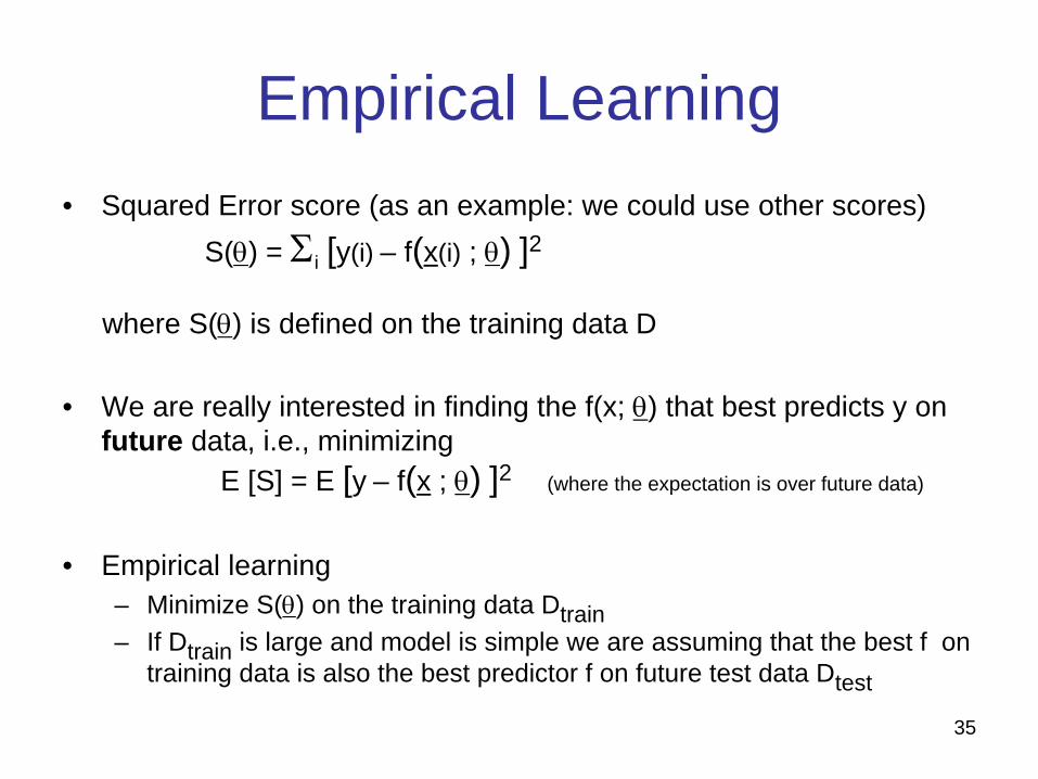
Empirical Learning• Squared Error score (as an example: we could use other scores)

S() = i [y(i) – f(x(i) ; ) ]2

where S() is defined on the training data D

• We are really interested in finding the f(x; ) that best predicts y on future data, i.e., minimizing

E [S] = E [y – f(x ; ) ]2 (where the expectation is over future data)

• Empirical learning– Minimize S() on the training data Dtrain– If Dtrain is large and model is simple we are assuming that the best f on

training data is also the best predictor f on future test data Dtest

36

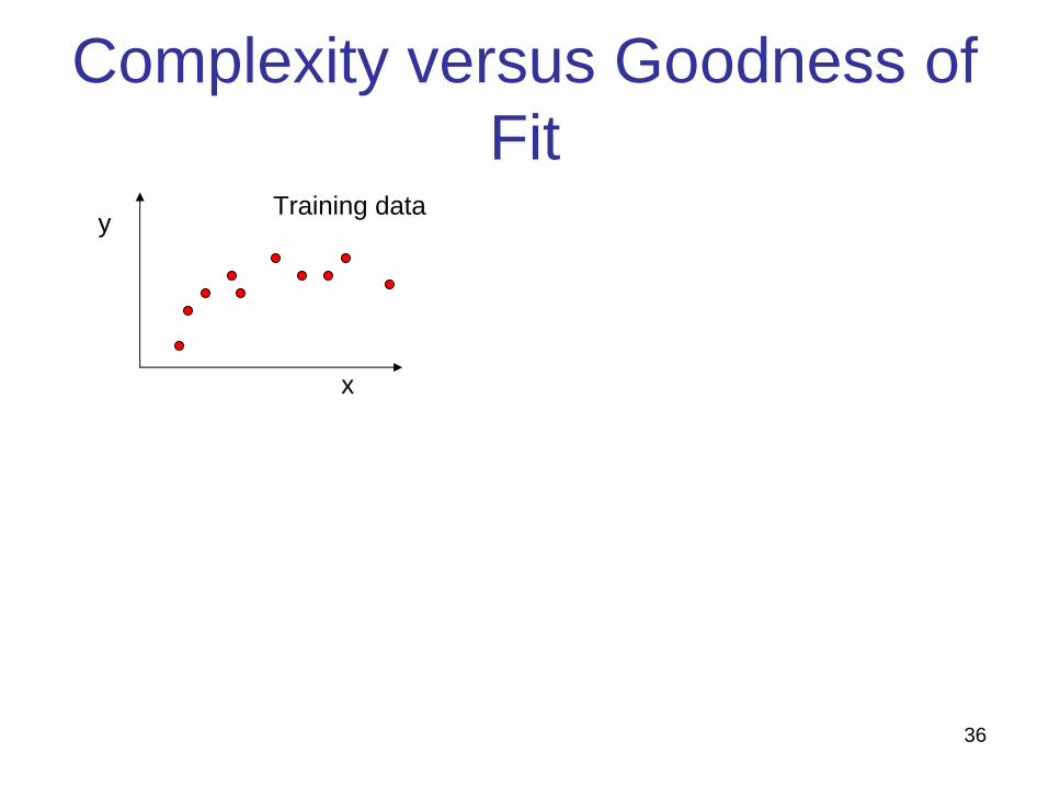
Complexity versus Goodness of Fit

x

yTraining data

37

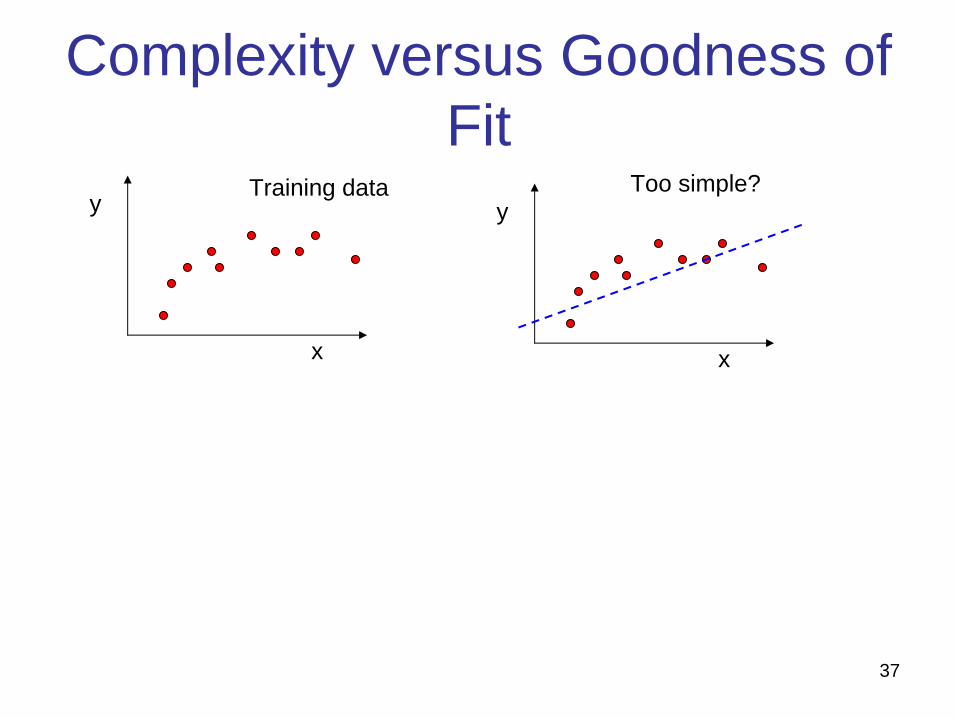
Complexity versus Goodness of Fit

x

y

x

yToo simple?Training data

38

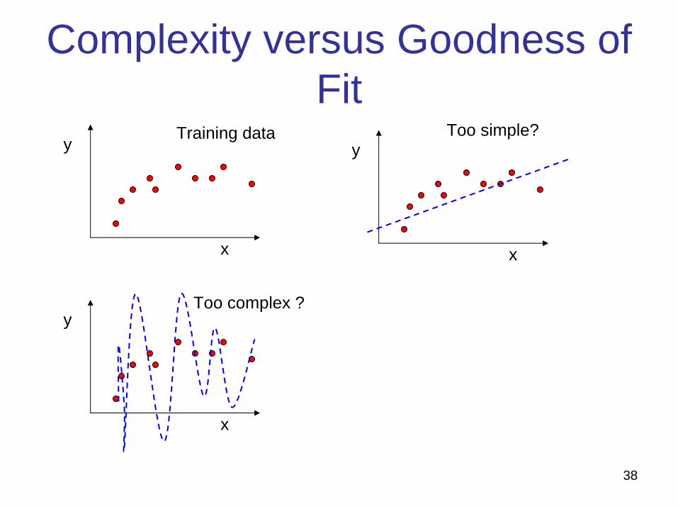
Complexity versus Goodness of Fit

x

y

x

y

x

y

Too simple?

Too complex ?

Training data

39

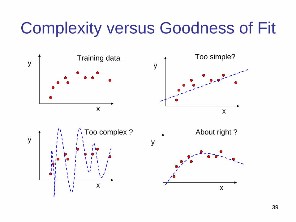
Complexity versus Goodness of Fit

x

y

x

y

x

y

x

y

Too simple?

Too complex ? About right ?

Training data

40

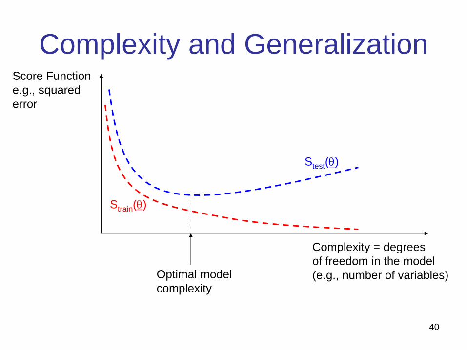
Complexity and Generalization

Strain ()

Stest ()

Complexity = degreesof freedom in the model(e.g., number of variables)

Score Functione.g., squarederror

Optimal modelcomplexity

41

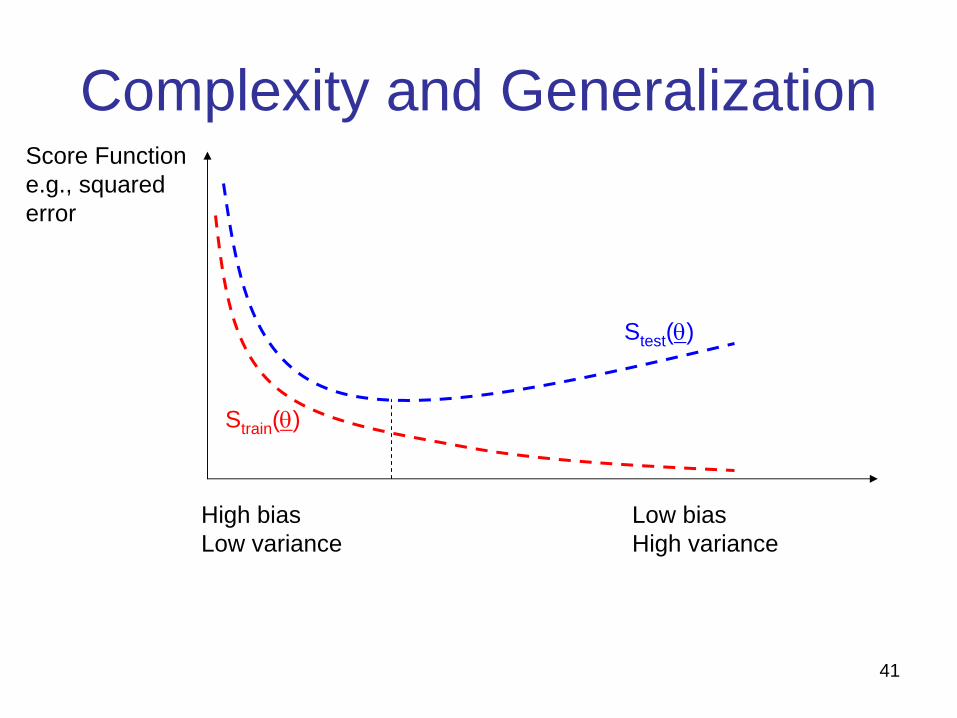
Complexity and Generalization

Strain ()

Stest ()

Score Functione.g., squarederror

High biasLow variance

Low biasHigh variance

42

Defining what “best” means• How do we measure “best”?

– Best performance on the training data?• K = p will be best (i.e., use all variables), e.g., p=10,000• So this is not useful in general

– Performance on the training data will in general be optimistic

• Practical Alternatives:– Measure performance on a single validation set

– Measure performance using multiple validation sets• Cross-validation

– Add a penalty term to the score function that “corrects” for optimism

• E.g., “regularized” regression: SSE +

sum of weights squared

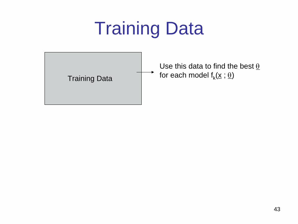
43

Training Data

Training DataUse this data to find the best

for each model fk (x ; )

44

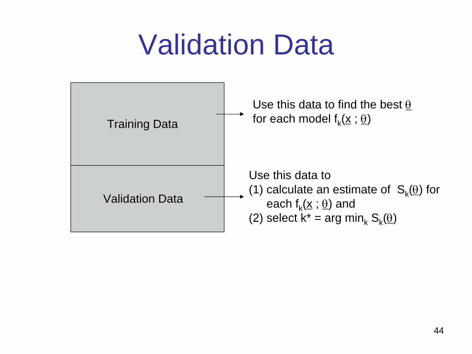
Validation Data

Training Data

Validation Data

Use this data to find the best

for each model fk (x ; )

Use this data to (1) calculate an estimate of Sk () for

each fk (x ; ) and (2) select k* = arg mink Sk ()

45

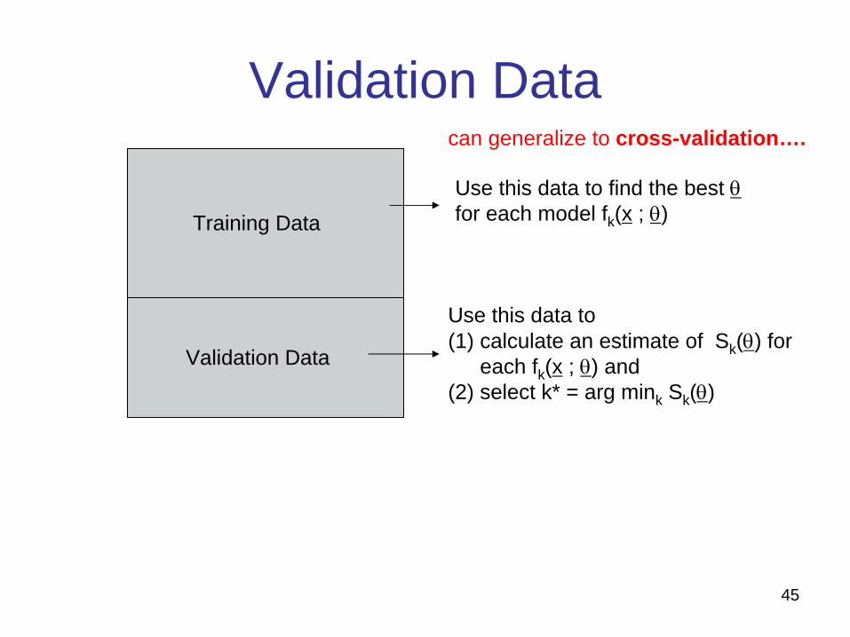
Validation Data

Training Data

Validation Data

Use this data to find the best

for each model fk (x ; )

Use this data to (1) calculate an estimate of Sk () for

each fk (x ; ) and (2) select k* = arg mink Sk ()

can generalize to cross-validation….

46

2 different (but related) issues here

1. Finding the function f that minimizes S() for future data

2. Getting a good estimate of S(), using the chosen function, on future data,– e.g., we might have selected the best function f, but our estimate

of its performance will be optimistically biased if our estimate of the score uses any of the same data used to fit and select the model.

47

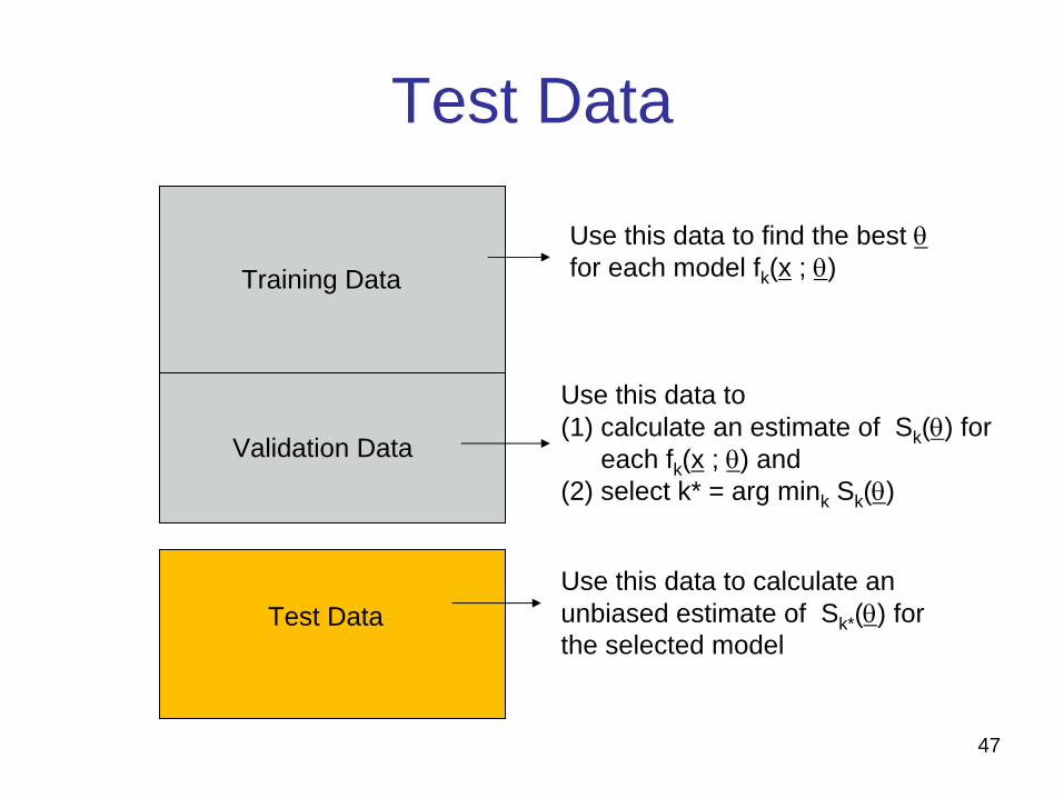
Test Data

Training Data

Validation Data

Test Data

Use this data to find the best

for each model fk (x ; )

Use this data to (1) calculate an estimate of Sk () for

each fk (x ; ) and (2) select k* = arg mink Sk ()

Use this data to calculate an unbiased estimate of Sk* () for the selected model

48

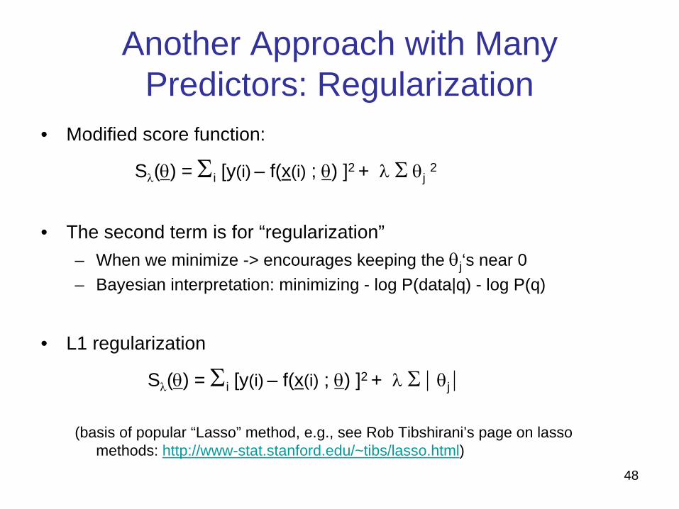
Another Approach with Many Predictors: Regularization

• Modified score function:

S

() = i [y(i) – f(x(i) ; ) ]2 +

j 2

• The second term is for “regularization”– When we minimize -> encourages keeping the j ‘s near 0– Bayesian interpretation: minimizing - log P(data|q) - log P(q)

• L1 regularization

S

() = i [y(i) – f(x(i) ; ) ]2 +

j

(basis of popular “Lasso” method, e.g., see Rob Tibshirani’s page on lasso methods: http://www-stat.stanford.edu/~tibs/lasso.html)

49

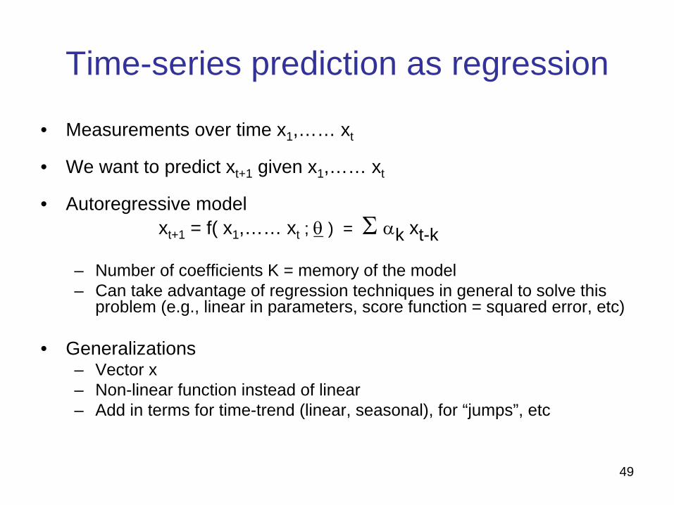
Time-series prediction as regression

• Measurements over time x1 ,…… xt

• We want to predict xt+1 given x1 ,…… xt

• Autoregressive model xt+1 = f( x1 ,…… xt ;

) =

k xt-k

– Number of coefficients K = memory of the model– Can take advantage of regression techniques in general to solve this

problem (e.g., linear in parameters, score function = squared error, etc)

• Generalizations– Vector x– Non-linear function instead of linear– Add in terms for time-trend (linear, seasonal), for “jumps”, etc

50

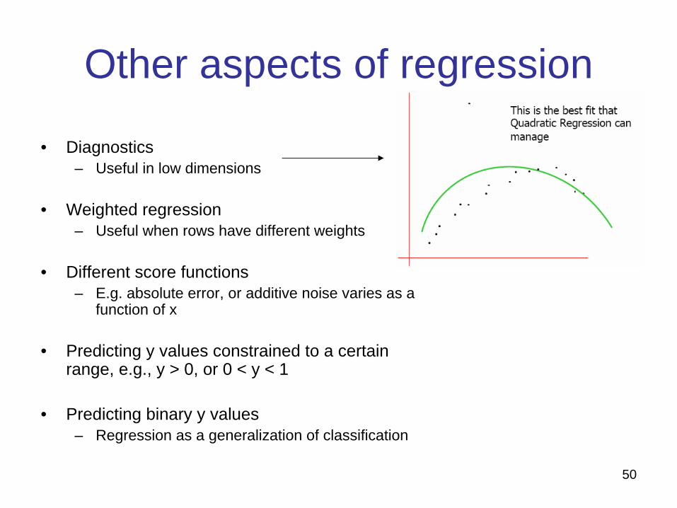
Other aspects of regression

• Diagnostics– Useful in low dimensions

• Weighted regression– Useful when rows have different weights

• Different score functions– E.g. absolute error, or additive noise varies as a

function of x

• Predicting y values constrained to a certain range, e.g., y > 0, or 0 < y < 1

• Predicting binary y values– Regression as a generalization of classification

51

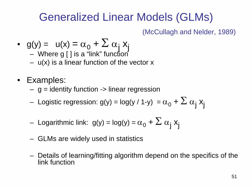
Generalized Linear Models (GLMs) (McCullagh and Nelder, 1989)

• g(y) = u(x) = 0 +

j xj– Where g [ ] is a “link” function– u(x) is a linear function of the vector x

• Examples:– g = identity function -> linear regression

– Logistic regression: g(y) = log(y / 1-y) = 0 +

j xj

– Logarithmic link: g(y) = log(y) = 0 +

j xj

– GLMs are widely used in statistics

– Details of learning/fitting algorithm depend on the specifics of the link function

52

Tree-Structured Regression• Functional form of model is a “regression tree”

– Univariate thresholds at internal nodes– Constant or linear surfaces at the leaf nodes– Yields piecewise constant (or linear) surface– (like classification tree, but for regression)

• Very crude functional form…. but– Can be very useful in high-dimensional problems– Can useful for interpretation– Can handle combinations of real and categorical variables

• Search problem– Finding the optimal tree is intractable– Practice: greedy algorithms

53

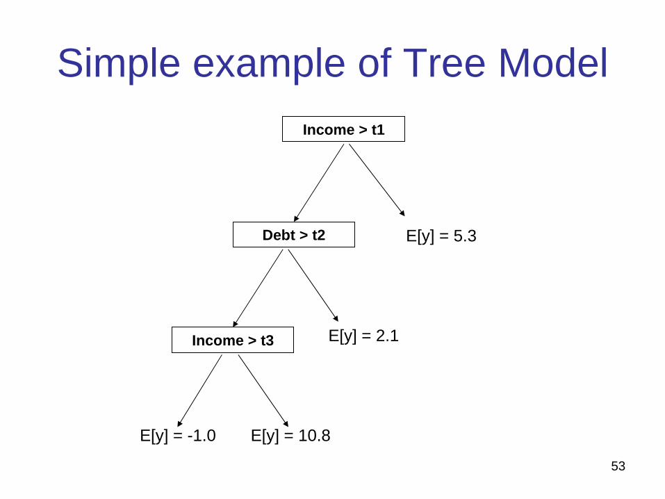
Simple example of Tree ModelIncome > t1

Debt > t2

Income > t3

E[y] = 5.3

E[y] = 2.1

E[y] = 10.8E[y] = -1.0

54

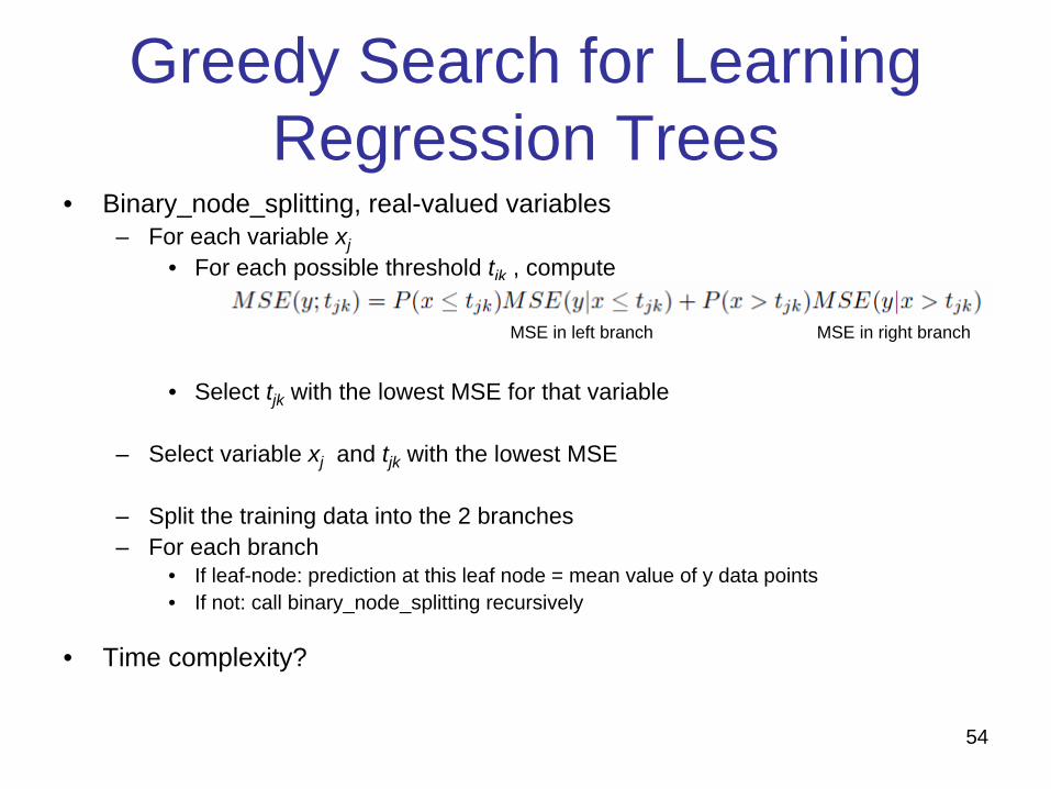
Greedy Search for Learning Regression Trees

• Binary_node_splitting, real-valued variables– For each variable xj

• For each possible threshold tjk , compute

• Select tjk with the lowest MSE for that variable

– Select variable xj and tjk with the lowest MSE

– Split the training data into the 2 branches– For each branch

• If leaf-node: prediction at this leaf node = mean value of y data points• If not: call binary_node_splitting recursively

• Time complexity?

MSE in left branch MSE in right branch

55

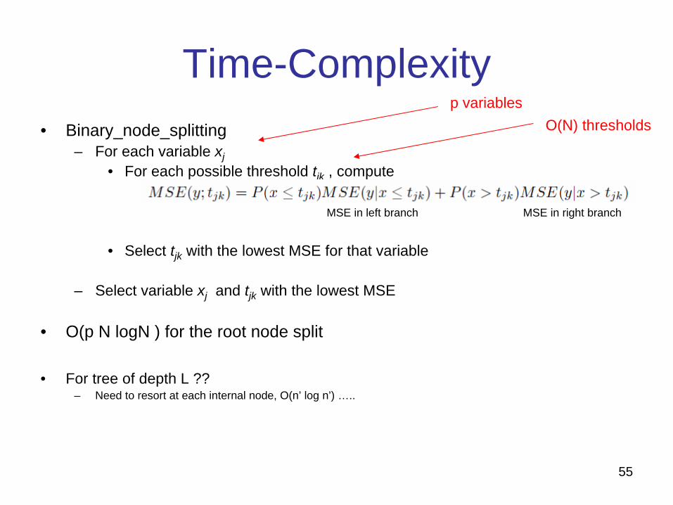
Time-Complexity • Binary_node_splitting

– For each variable xj• For each possible threshold tjk , compute

• Select tjk with the lowest MSE for that variable

– Select variable xj and tjk with the lowest MSE

• O(p N logN ) for the root node split

• For tree of depth L ??– Need to resort at each internal node, O(n’ log n’) …..

MSE in left branch MSE in right branch

p variablesO(N) thresholds

56

More on Regression Trees• Greedy search algorithm

– For each variable, find the best split point such the mean of Y either side of the split minimizes the mean-squared error

– Select the variable with the minimum average error• Partition the data using the threshold

– Recursively apply this selection procedure to each “branch”

• What size tree?– A full tree will likely overfit the data– Common methods for tree selection

• Grow a large tree and select an appropriate subtree by Xvalidation• Grow a number of small fixed-sized trees and average their predictions

• Will discuss trees further in lectures on classification: very similar ideas used for building classification trees and regression trees

57

Model Averaging• Can average over parameters and models

– E.g., weighted linear combination of predictions from multiple models

y =

wk yk

– Why? Any predictions from a point estimate of parameters or a single model has only a small chance of the being the best

– Averaging makes our predictions more stable and less sensitive to random variations in a particular data set (good for less stable models like trees)

58

Model Averaging• Model averaging flavors

– Fully Bayesian: average over uncertainty in parameters and models

– “empirical Bayesian”: learn weights over multiple models• E.g., stacking and bagging (widely used in Netflix competition)

– Build multiple simple models in a systematic way and combine them, e.g.,

• Boosting: will say more about this in later lectures

• Random forests (for trees): stochastically perturb the data, learn multiple trees, and then combine for prediction

59

Components of ML Algorithms

• Model Representation:– Determining the nature and structure of the representation to be used

• Score function– Measuring how well different representations fit the data

• Search/Optimization method– An algorithm to optimize the score function

• Data Management– Deciding what principles of data management are required to implement

the algorithms efficiently.

60

Software• MATLAB

– Many free “toolboxes” on the Web for regression and prediction– e.g., see http://lib.stat.cmu.edu/matlab/

and in particular the CompStats toolbox

• R– General purpose statistical computing environment (successor to S)– Free (!)– Widely used by statisticians, has a huge library of functions and

visualization tools

• Commercial tools– SAS, Salford Systems, other statistical packages– Various data mining packages– Often are not programmable: offer a fixed menu of items

61

Useful References

N. R. Draper and H. Smith, Applied Regression Analysis, 2nd edition,Wiley, 1981(the “bible” for classical regression methods in statistics)

T. Hastie, R. Tibshirani, and J. Friedman, Elements of Statistical Learning, 2nd edition,Springer Verlag, 2009(statistically-oriented overview of modern ideas in regression and classification, mixes machine learning and statistics)