CS-184: Computer Graphics Lecture #20: Fluid Simulation I

Rahul NarainUniversity of California, Berkeley!Nov. 18, 2013

Fluids

Kim, Thuerey, James, and Gross, 2008

Fluids

Losasso, Talton, Kwatra, and Fedkiw, 2008

Fluids

Feldman, O’Brien, and Arikan, 2003

Two ways of representing flow

Particles

Grid

“Lagrangian”

“Eulerian”J.-L. Lagrange

(dead now)L. Euler

(also dead)

Smoothed particle hydrodynamics (SPH)

• Each particle has mass, position, velocity

• Particles represent samples of continuous underlying scalar/vector fields (density, velocity, etc.)

v(x) = ?•x

x1v1

x2 v2 v3

x4 v4

x3

SPH interpolation

• Evaluate the field anywhere by weighted averaging

Value at point x

Value at particle i “Volume” of particle i

Smoothing kernel

A(x) =X

i

Aimi

⇢iW (x� xi)

††x - xi§§

W

⇢i := ⇢(xi) =X

j

mjW (xi � xj)Density:

Particle-based fluids

• Each particle has a velocity

• Each time step:

• Compute acceleration a of each particle

• Update velocities: v = v + a dt

• Update positions: x = x + v dtLeapfrog integration}

Forces?

External forces

• E.g. gravity

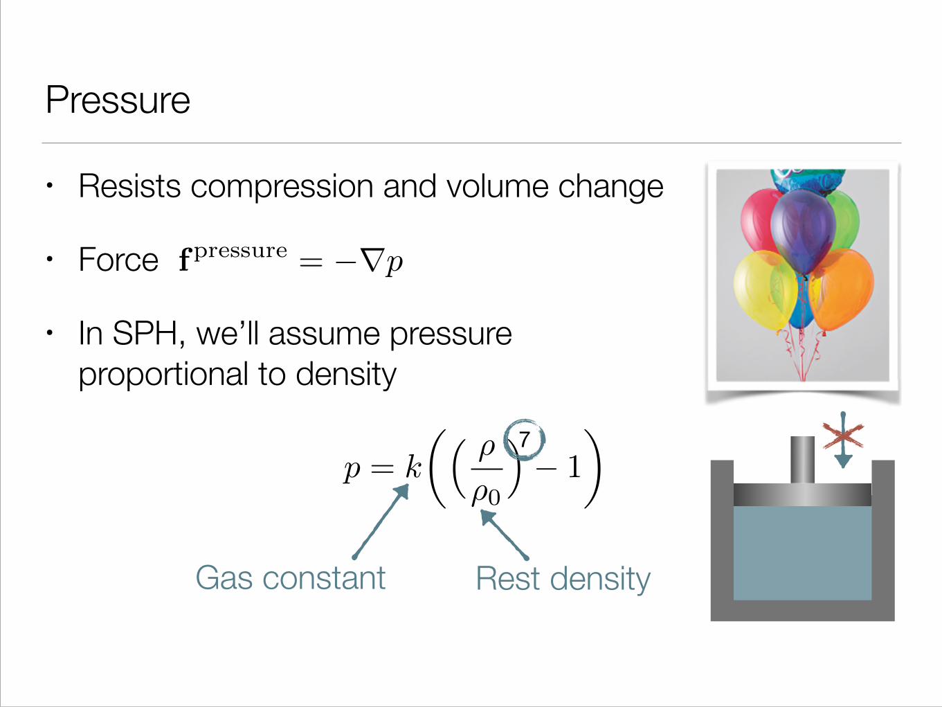
Pressure

• Resists compression and volume change

• Force

• In SPH, we’ll assume pressure proportional to density

p = k

✓⇣ ⇢

⇢0

⌘� 1

◆

Rest density

fpressure = �rp

7

Gas constant

Pressure

Becker and Teschner, 2007

Viscosity

• Resists relative motion within the fluid

fviscosity = µr2v

Coefficient of viscosity

Surface tension

• Tries to minimize surface area

• Only relevant at small scales

• Hard to do correctly

Forces in a fluid

• Forces (per unit volume)

!

!

• How to evaluate gradients of quantities?

f = ⇢g �rp+ µr2v

Gravity

Pressure

Viscosity

Evaluating gradients with SPH

!

• So

!

• We just have to differentiate the kernel!

• Same thing works for higher derivatives (for viscosity).

A(x) =X

i

Aimi

⇢iW (x� xi)

rA(x) =X

i

Aimi

⇢irW (x� xi)

Newton’s third law

• Forces between two particles should be equal & opposite

f

viscosity

i = µX

j

vjmj

⇢jr2W (xi � xj)

f

pressurei = �

X

j

pjmj

⇢jrW (xi � xj)

Newton’s third law

• Forces between two particles should be equal & opposite

f

pressurei = �

X

j

⇣pi + pj2

⌘mj

⇢jrW (xi � xj)

f

viscosity

i = µX

j

(vj � vi)mj

⇢jr2W (xi � xj)

Putting it all together

• For each particle:

• Compute ⍴i for each particle

• For each particle:

• Evaluate net force fi

• Compute acceleration

• Perform leapfrog integration

ai = fi/⇢i

Particles

Akinci, Ihmsen, Akinci, Solenthaler, and Teschner, 2010

Particles

Akinci, Ihmsen, Akinci, Solenthaler, and Teschner, 2010

Surface reconstruction

• Define a “color function” c(x) that is 1 inside the fluid and 0 outside

• e.g. do SPH interpolation as usual with ci = 1 always

!

• Extract isosurface at c = ½

c(x) =X

i

cimj

⇢jW (x� xj)

Surface reconstruction

• Surface can look “lumpy” due to particle distribution

• Solution: use anisotropic kernels along surface

Isotropic kernels Anisotropic kernelsYu and Turk, 2010

Smoothed particle hydrodynamics!

Akinci, Ihmsen, Akinci, Solenthaler, and Teschner, 2010

References

• Müller, Charypar, and Gross, “Particle-Based Fluid Simulation for Interactive Applications”, 2003

• Becker and Teschner, “Weakly compressible SPH for free surface flows”, 2007

• Yu and Turk, “Reconstructing Surfaces of Particle-Based Fluids Using Anisotropic Kernels”, 2010