1

CS 188: Artificial IntelligenceFall 2007

Lecture 22: Viterbi

11/13/2007

Dan Klein – UC Berkeley

Hidden Markov Models

� An HMM is� Initial distribution:

� Transitions:

� Emissions:

X5X2

E1

X1 X3 X4

E2 E3 E4 E5

2

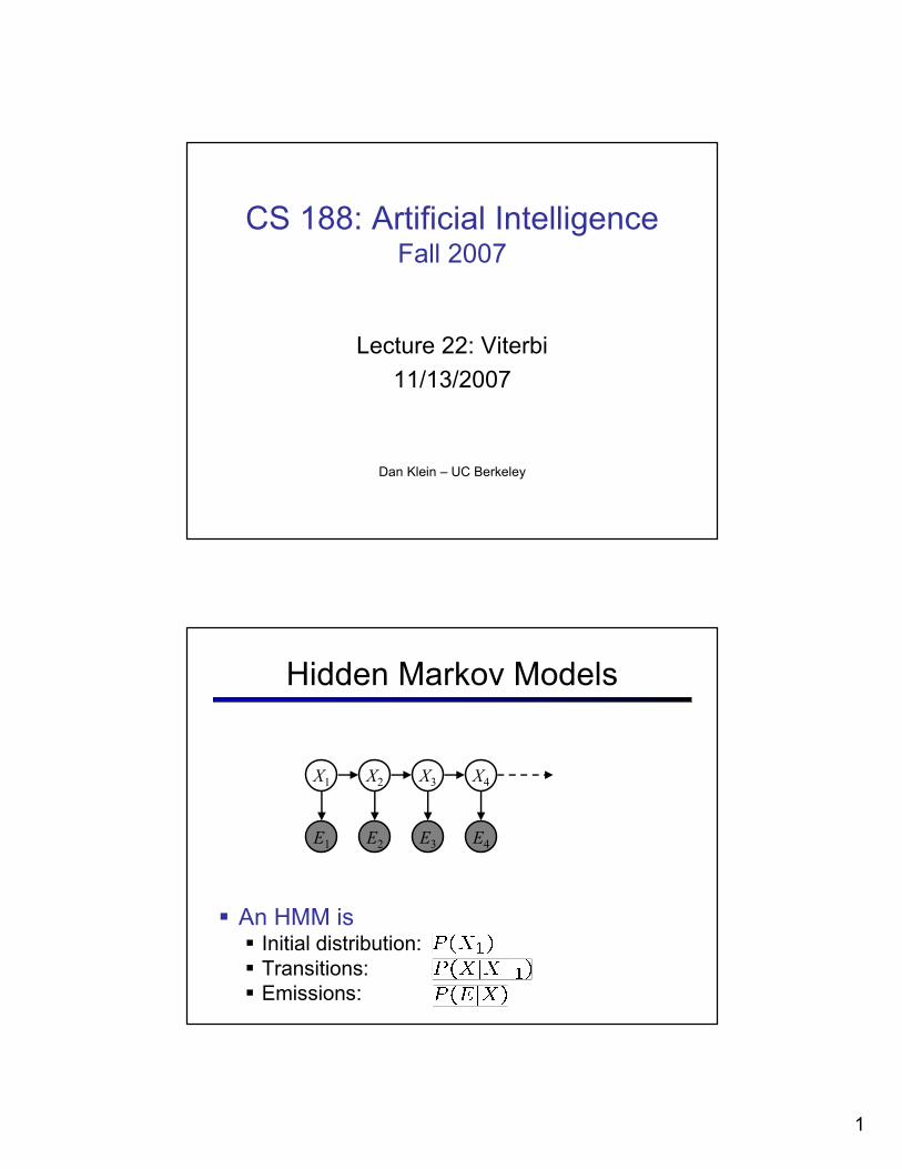
Most Likely Explanation

� Remember: weather Markov chain

� Tracking:

� Viterbi:

sun

rain

sun

rain

sun

rain

sun

rain

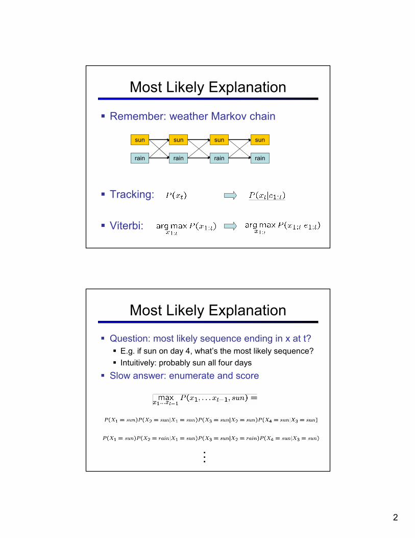
Most Likely Explanation

� Question: most likely sequence ending in x at t?

� E.g. if sun on day 4, what’s the most likely sequence?

� Intuitively: probably sun all four days

� Slow answer: enumerate and score

…

3

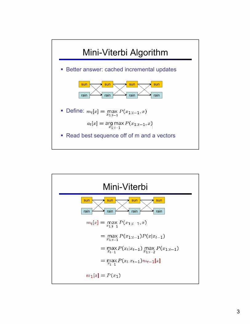
Mini-Viterbi Algorithm

� Better answer: cached incremental updates

� Define:

� Read best sequence off of m and a vectors

sun

rain

sun

rain

sun

rain

sun

rain

Mini-Viterbi

sun

rain

sun

rain

sun

rain

sun

rain

4

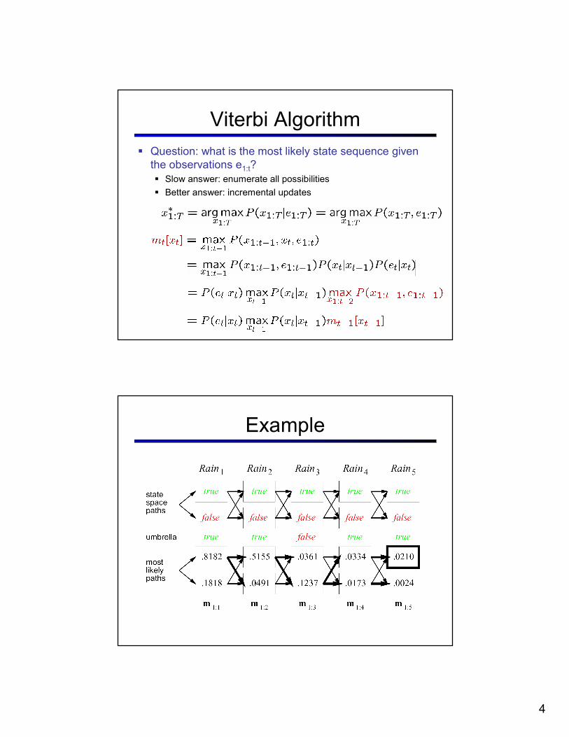
Viterbi Algorithm

� Question: what is the most likely state sequence given

the observations e1:t?

� Slow answer: enumerate all possibilities

� Better answer: incremental updates

Example

5

Digitizing Speech

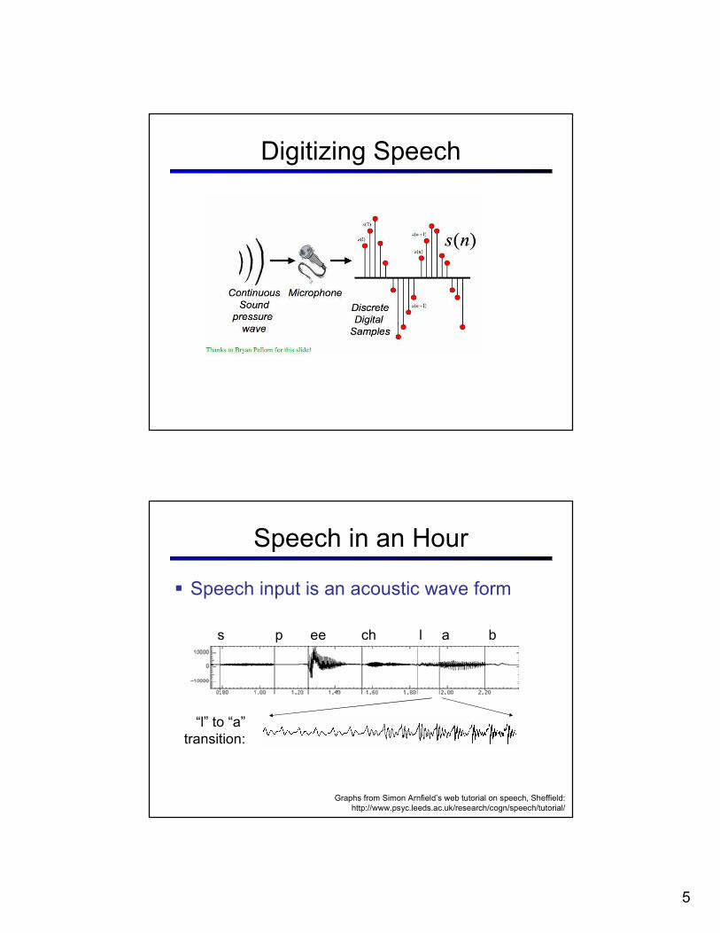
Speech in an Hour

� Speech input is an acoustic wave form

s p ee ch l a b

Graphs from Simon Arnfield’s web tutorial on speech, Sheffield:

http://www.psyc.leeds.ac.uk/research/cogn/speech/tutorial/

“l” to “a”

transition:

6

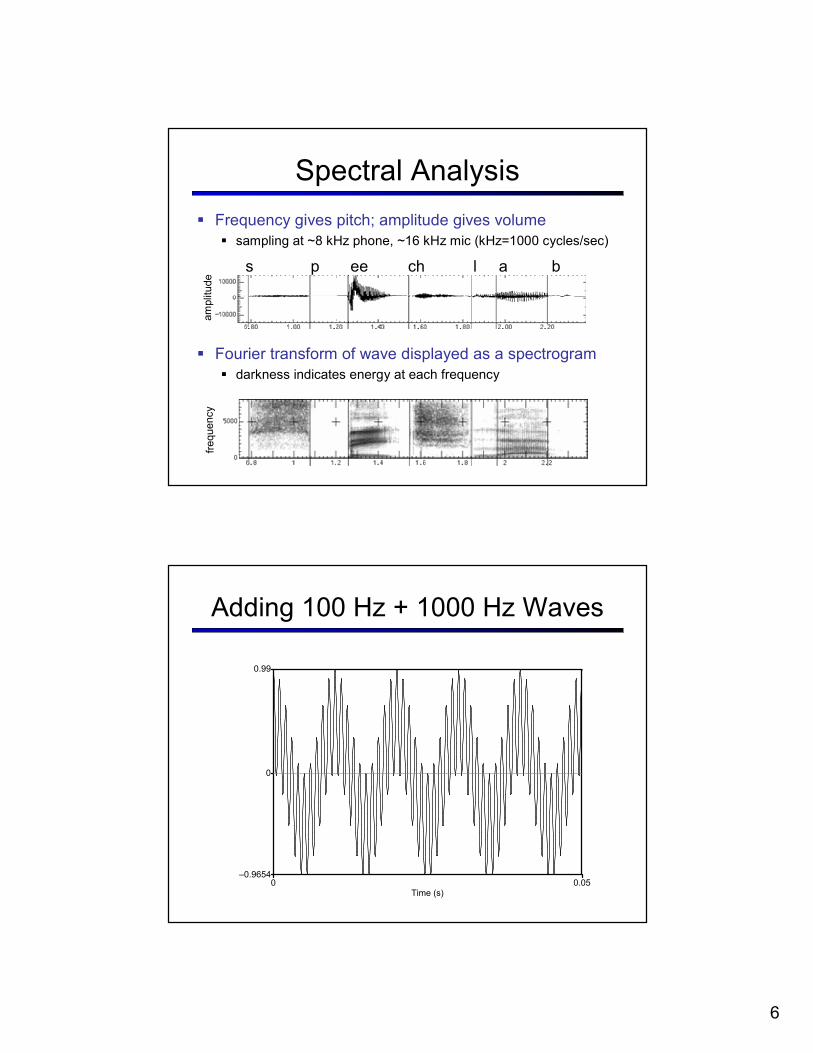
� Frequency gives pitch; amplitude gives volume

� sampling at ~8 kHz phone, ~16 kHz mic (kHz=1000 cycles/sec)

� Fourier transform of wave displayed as a spectrogram

� darkness indicates energy at each frequency

s p ee ch l a b

frequency

amplitude

Spectral Analysis

Adding 100 Hz + 1000 Hz Waves

Time (s)0 0.05

–0.9654

0.99

0

7

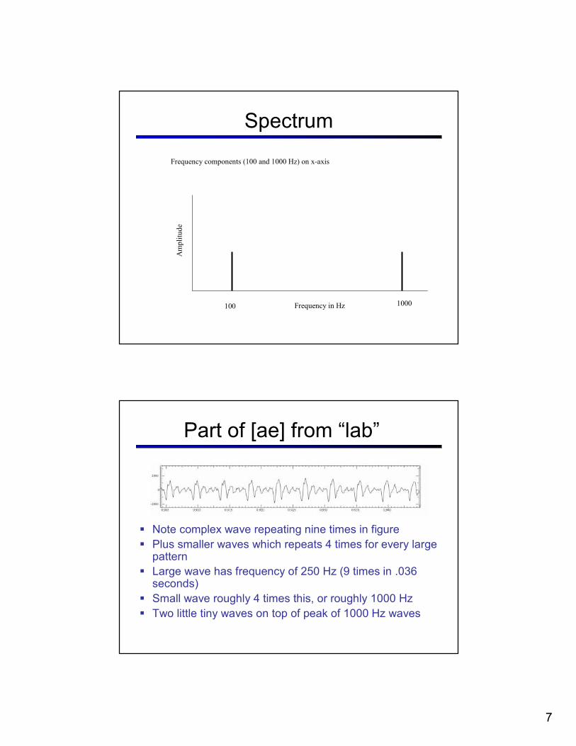
Spectrum

100 1000Frequency in Hz

Amplitude

Frequency components (100 and 1000 Hz) on x-axis

Part of [ae] from “lab”

� Note complex wave repeating nine times in figure

� Plus smaller waves which repeats 4 times for every large pattern

� Large wave has frequency of 250 Hz (9 times in .036 seconds)

� Small wave roughly 4 times this, or roughly 1000 Hz

� Two little tiny waves on top of peak of 1000 Hz waves

8

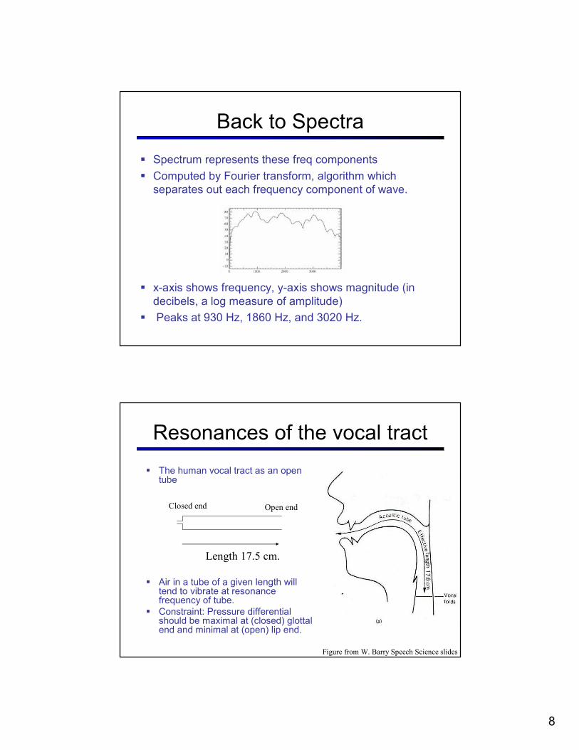
Back to Spectra

� Spectrum represents these freq components

� Computed by Fourier transform, algorithm which

separates out each frequency component of wave.

� x-axis shows frequency, y-axis shows magnitude (in

decibels, a log measure of amplitude)

� Peaks at 930 Hz, 1860 Hz, and 3020 Hz.

Resonances of the vocal tract

� The human vocal tract as an open tube

� Air in a tube of a given length will tend to vibrate at resonance frequency of tube.

� Constraint: Pressure differential should be maximal at (closed) glottal end and minimal at (open) lip end.

Closed end Open end

Length 17.5 cm.

Figure from W. Barry Speech Science slides

9

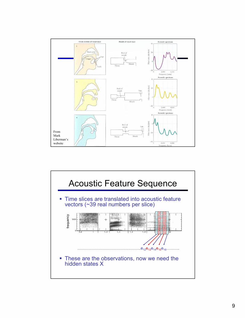
From

Mark

Liberman’s

website

Acoustic Feature Sequence

� Time slices are translated into acoustic feature vectors (~39 real numbers per slice)

� These are the observations, now we need the hidden states X

frequency

……………………………………………..e12e13e14e15e16………..

10

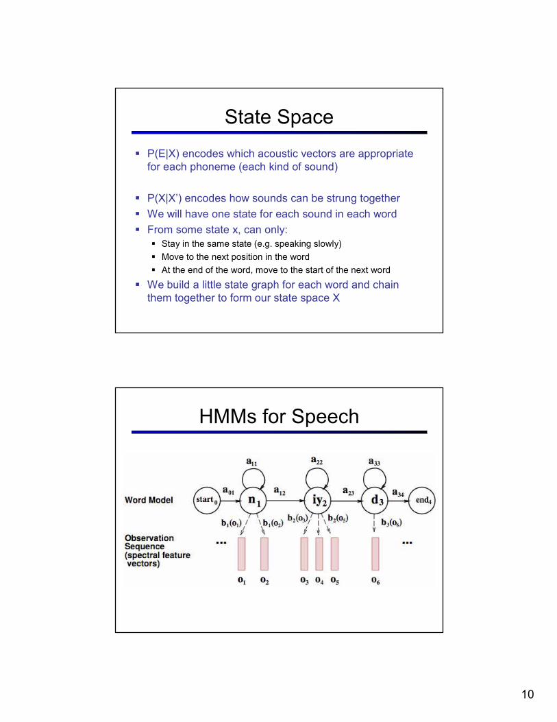
State Space

� P(E|X) encodes which acoustic vectors are appropriate

for each phoneme (each kind of sound)

� P(X|X’) encodes how sounds can be strung together

� We will have one state for each sound in each word

� From some state x, can only:

� Stay in the same state (e.g. speaking slowly)

� Move to the next position in the word

� At the end of the word, move to the start of the next word

� We build a little state graph for each word and chain

them together to form our state space X

HMMs for Speech

11

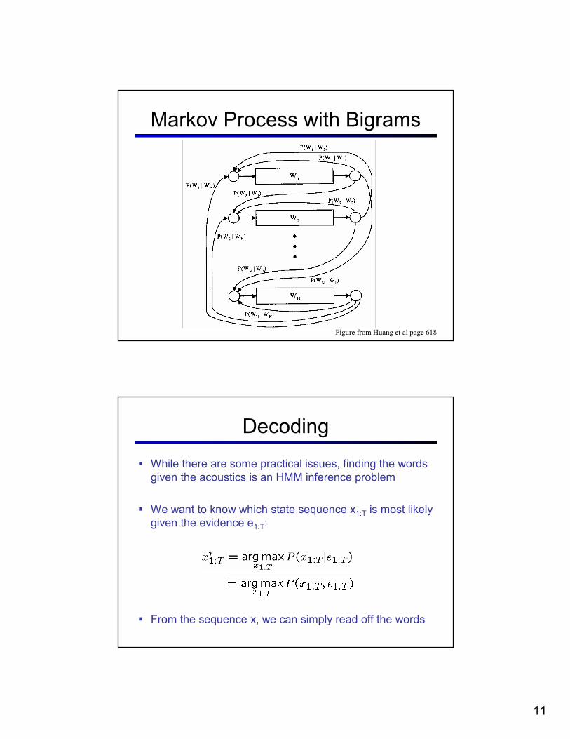
Markov Process with Bigrams

Figure from Huang et al page 618

Decoding

� While there are some practical issues, finding the words

given the acoustics is an HMM inference problem

� We want to know which state sequence x1:T is most likely

given the evidence e1:T:

� From the sequence x, we can simply read off the words

12

POMDPs

� Up until now:� MDPs: decision making when the world is fully observable (even if the actions are non-deterministic

� Probabilistic reasoning: computing beliefs in a static world

� What about acting under uncertainty?� In general, the formalization of the problem is the partially observable Markov decision process (POMDP)

� A simple case: value of information

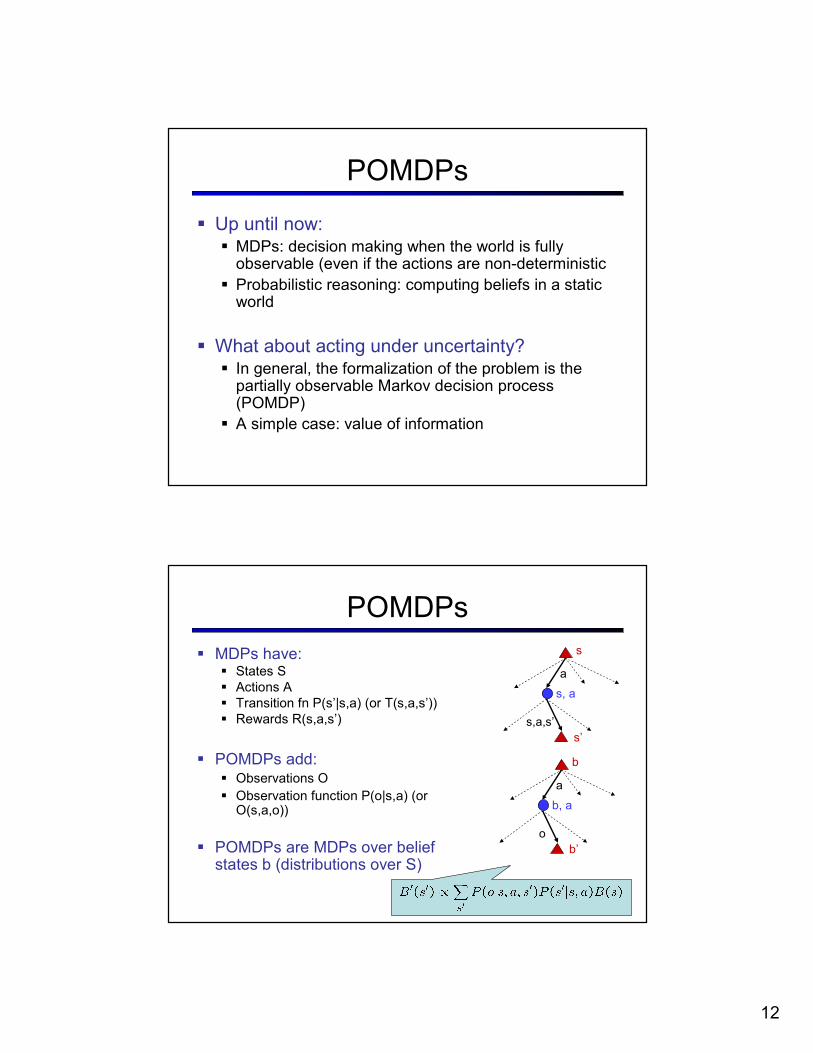
POMDPs

� MDPs have:� States S

� Actions A

� Transition fn P(s’|s,a) (or T(s,a,s’))

� Rewards R(s,a,s’)

� POMDPs add:� Observations O

� Observation function P(o|s,a) (or O(s,a,o))

� POMDPs are MDPs over belief states b (distributions over S)

a

s

s, a

s,a,s’

s’

a

b

b, a

o

b’

13

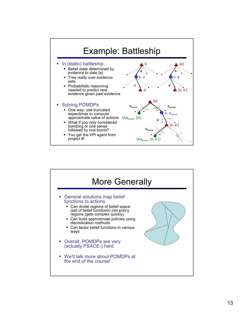
Example: Battleship

� In (static) battleship:� Belief state determined by evidence to date {e}

� Tree really over evidence sets

� Probabilistic reasoning needed to predict new evidence given past evidence

� Solving POMDPs� One way: use truncated expectimax to compute approximate value of actions

� What if you only considered bombing or one sense followed by one bomb?

� You get the VPI agent from project 4!

a

{e}

e, a

e’

{e, e’}

a

b

b, a

o

b’

abomb

{e}

e, asense

e’

{e, e’}

asense

U(abomb, {e})

abomb

U(abomb, {e, e’})

More Generally

� General solutions map belief functions to actions� Can divide regions of belief space (set of belief functions) into policy regions (gets complex quickly)

� Can build approximate policies using discretization methods

� Can factor belief functions in various ways

� Overall, POMDPs are very (actually PSACE-) hard

� We’ll talk more about POMDPs at the end of the course!