Embed Size (px)
Citation preview
CS 252 Graduate Computer Architecture
Lecture 2 - Metrics and Pipelining
Krste AsanovicElectrical Engineering and Computer Sciences
University of California at Berkeley
http://www.eecs.berkeley.edu/~krste
http://inst.eecs.berkeley.edu/~cs252
8/30 CS252-Fall!07 2
Review from Last Time
• Computer Architecture >> instruction sets
• Computer Architecture skill sets are different– 5 Quantitative principles of design
– Quantitative approach to design
– Solid interfaces that really work
– Technology tracking and anticipation
• CS 252 to learn new skills, transition to research
• Computer Science at the crossroads from sequentialto parallel computing
– Salvation requires innovation in many fields, including computerarchitecture
• Opportunity for interesting and timely CS 252projects exploring CS at the crossroads
– RAMP as experimental platform
8/30 CS252-Fall!07 3
Review (continued)
• Other fields often borrow ideas from architecture
• Quantitative Principles of Design1. Take Advantage of Parallelism
2. Principle of Locality
3. Focus on the Common Case
4. Amdahl’s Law
5. The Processor Performance Equation
• Careful, quantitative comparisons– Define, quantity, and summarize relative performance
– Define and quantity relative cost
– Define and quantity dependability
– Define and quantity power
• Culture of anticipating and exploiting advances intechnology
• Culture of well-defined interfaces that are carefullyimplemented and thoroughly checked
8/30 CS252-Fall!07 4
Metrics used to Compare Designs
• Cost– Die cost and system cost
• Execution Time– average and worst-case
– Latency vs. Throughput
• Energy and Power– Also peak power and peak switching current
• Reliability– Resiliency to electrical noise, part failure
– Robustness to bad software, operator error
• Maintainability– System administration costs
• Compatibility– Software costs dominate
8/30 CS252-Fall!07 5
Cost of Processor
• Design cost (Non-recurring Engineering Costs, NRE)– dominated by engineer-years (~$200K per engineer year)
– also mask costs (exceeding $1M per spin)
• Cost of die– die area
– die yield (maturity of manufacturing process, redundancy features)
– cost/size of wafers
– die cost ~= f(die area^4) with no redundancy
• Cost of packaging– number of pins (signal + power/ground pins)
– power dissipation
• Cost of testing– built-in test features?
– logical complexity of design
– choice of circuits (minimum clock rates, leakage currents, I/O drivers)
Architect affects all of these
8/30 CS252-Fall!07 6
System-Level Cost Impacts
• Power supply and cooling
• Support chipset
• Off-chip SRAM/DRAM/ROM
• Off-chip peripherals
8/30 CS252-Fall!07 7
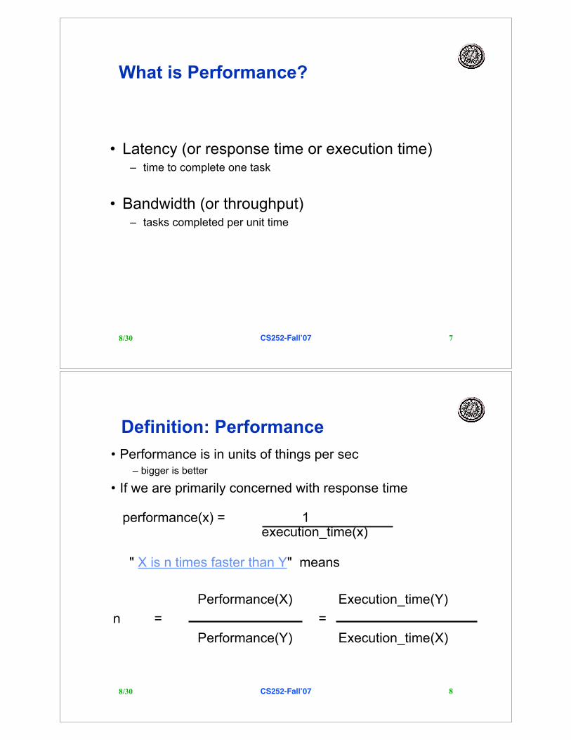
What is Performance?
• Latency (or response time or execution time)– time to complete one task
• Bandwidth (or throughput)– tasks completed per unit time
8/30 CS252-Fall!07 8
Performance(X) Execution_time(Y)
n = =
Performance(Y) Execution_time(X)
Definition: Performance
• Performance is in units of things per sec– bigger is better
• If we are primarily concerned with response time
performance(x) = 1 execution_time(x)
" X is n times faster than Y" means
8/30 CS252-Fall!07 9
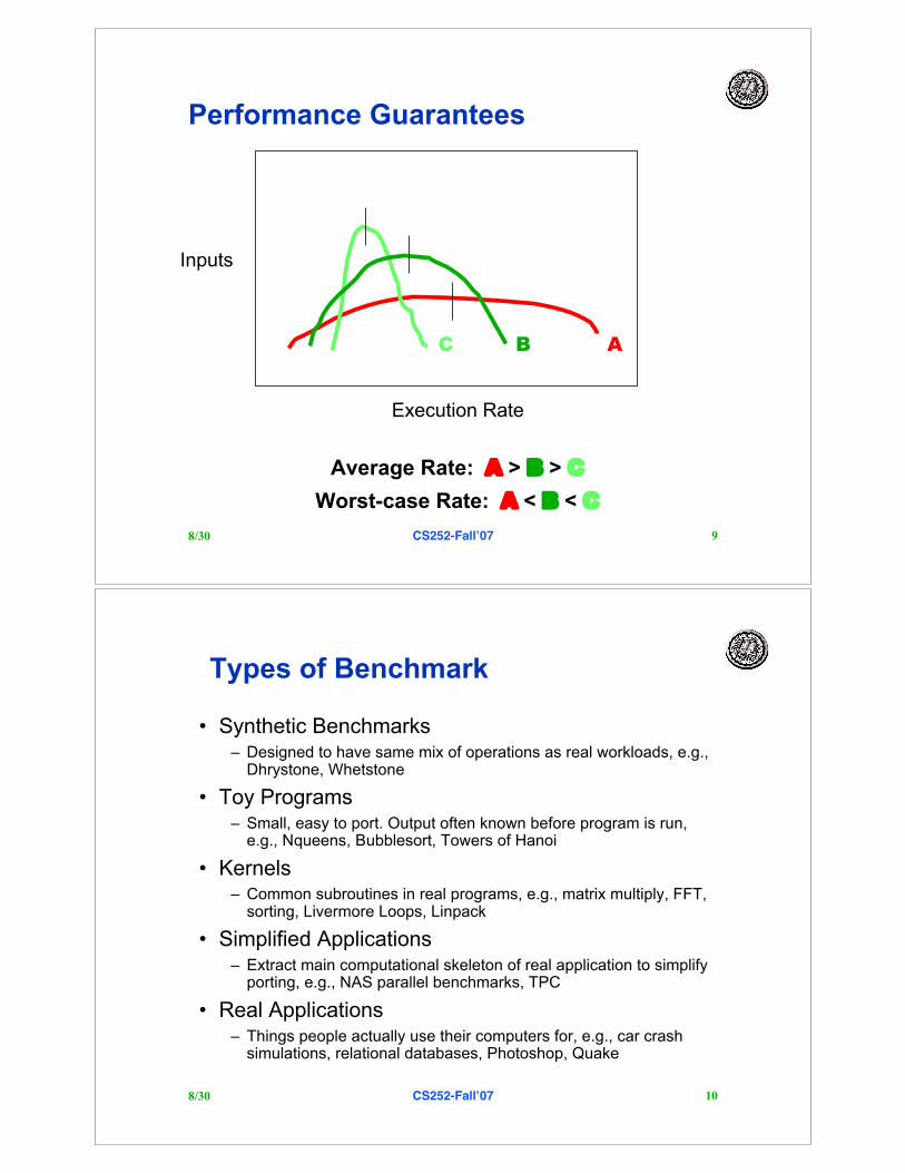
Performance Guarantees
A
Average Rate: A > B > C
Worst-case Rate: A < B < C
BC
Execution Rate
Inputs
8/30 CS252-Fall!07 10
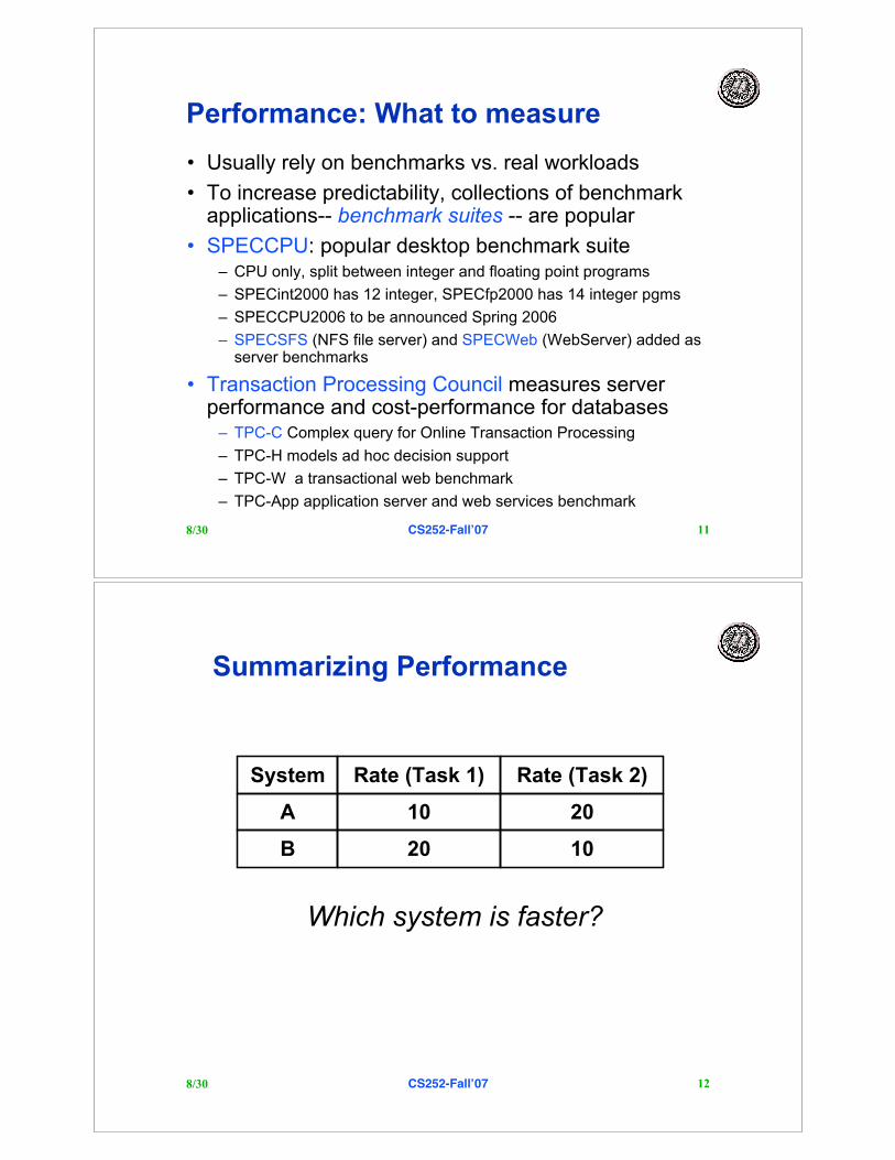
Types of Benchmark
• Synthetic Benchmarks– Designed to have same mix of operations as real workloads, e.g.,
Dhrystone, Whetstone
• Toy Programs– Small, easy to port. Output often known before program is run,
e.g., Nqueens, Bubblesort, Towers of Hanoi
• Kernels– Common subroutines in real programs, e.g., matrix multiply, FFT,
sorting, Livermore Loops, Linpack
• Simplified Applications– Extract main computational skeleton of real application to simplify
porting, e.g., NAS parallel benchmarks, TPC
• Real Applications– Things people actually use their computers for, e.g., car crash
simulations, relational databases, Photoshop, Quake
8/30 CS252-Fall!07 11
Performance: What to measure
• Usually rely on benchmarks vs. real workloads
• To increase predictability, collections of benchmarkapplications-- benchmark suites -- are popular
• SPECCPU: popular desktop benchmark suite– CPU only, split between integer and floating point programs
– SPECint2000 has 12 integer, SPECfp2000 has 14 integer pgms
– SPECCPU2006 to be announced Spring 2006
– SPECSFS (NFS file server) and SPECWeb (WebServer) added asserver benchmarks
• Transaction Processing Council measures serverperformance and cost-performance for databases
– TPC-C Complex query for Online Transaction Processing
– TPC-H models ad hoc decision support
– TPC-W a transactional web benchmark
– TPC-App application server and web services benchmark
8/30 CS252-Fall!07 12
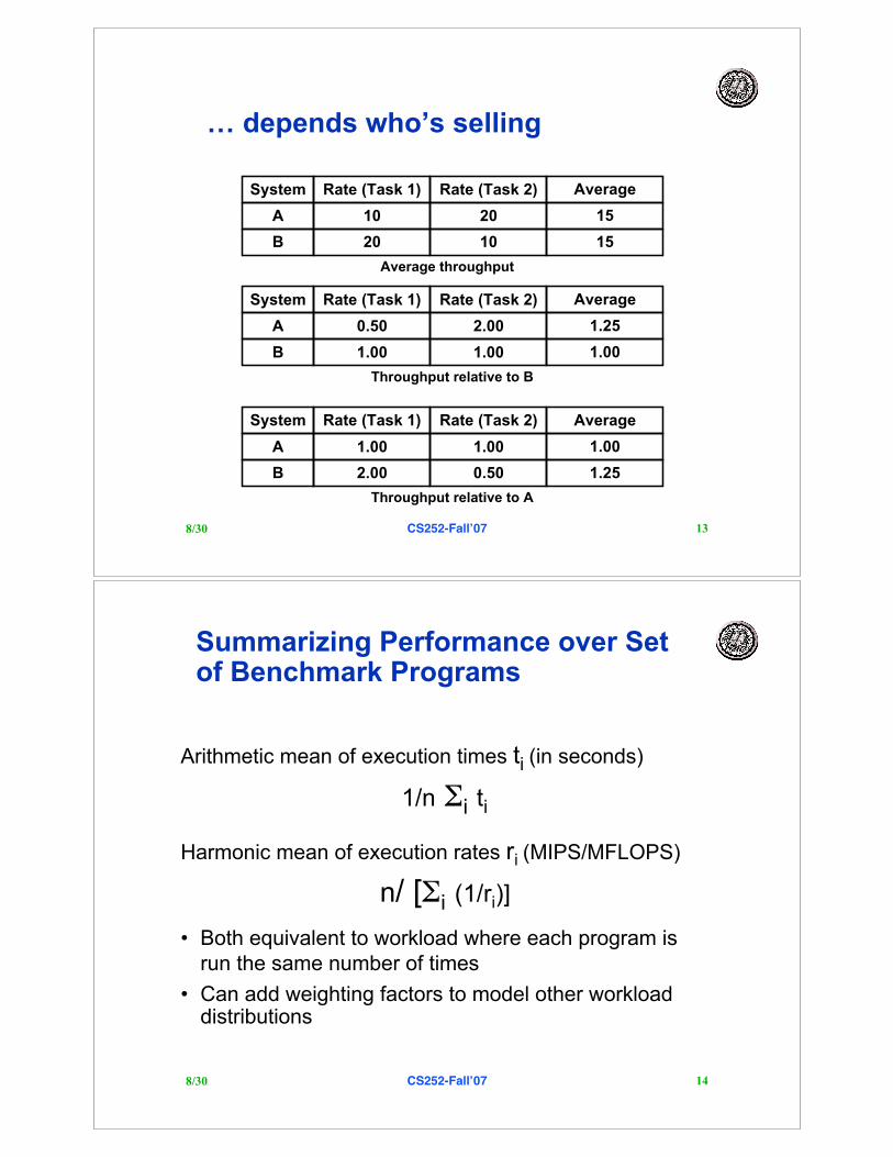
Summarizing Performance
Which system is faster?
System Rate (Task 1) Rate (Task 2)
A 10 20
B 20 10
8/30 CS252-Fall!07 13
… depends who’s selling
System Rate (Task 1) Rate (Task 2)
A 10 20
B 20 10
Average
15
15
Average throughput
System Rate (Task 1) Rate (Task 2)
A 0.50 2.00
B 1.00 1.00
Average
1.25
1.00
Throughput relative to B
System Rate (Task 1) Rate (Task 2)
A 1.00 1.00
B 2.00 0.50
Average
1.00
1.25
Throughput relative to A
8/30 CS252-Fall!07 14
Summarizing Performance over Setof Benchmark Programs
Arithmetic mean of execution times ti (in seconds)
1/n !i ti
Harmonic mean of execution rates ri (MIPS/MFLOPS)
n/ [!i (1/ri)]
• Both equivalent to workload where each program isrun the same number of times
• Can add weighting factors to model other workloaddistributions
8/30 CS252-Fall!07 15
Normalized Execution Timeand Geometric Mean
• Measure speedup up relative to reference machine
ratio = tRef/tA• Average time ratios using geometric mean
n"(#I ratioi )
• Insensitive to machine chosen as reference
• Insensitive to run time of individual benchmarks
• Used by SPEC89, SPEC92, SPEC95, …, SPEC2006
….. But beware that choice of reference machine cansuggest what is “normal” performance profile:
8/30 CS252-Fall!07 16
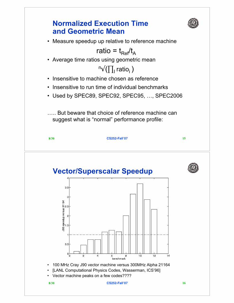
Vector/Superscalar Speedup
• 100 MHz Cray J90 vector machine versus 300MHz Alpha 21164
• [LANL Computational Physics Codes, Wasserman, ICS’96]
• Vector machine peaks on a few codes????
8/30 CS252-Fall!07 17
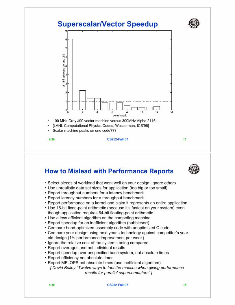
Superscalar/Vector Speedup
• 100 MHz Cray J90 vector machine versus 300MHz Alpha 21164
• [LANL Computational Physics Codes, Wasserman, ICS’96]
• Scalar machine peaks on one code???
8/30 CS252-Fall!07 18
How to Mislead with Performance Reports
• Select pieces of workload that work well on your design, ignore others• Use unrealistic data set sizes for application (too big or too small)• Report throughput numbers for a latency benchmark• Report latency numbers for a throughput benchmark• Report performance on a kernel and claim it represents an entire application• Use 16-bit fixed-point arithmetic (because it’s fastest on your system) even
though application requires 64-bit floating-point arithmetic• Use a less efficient algorithm on the competing machine• Report speedup for an inefficient algorithm (bubblesort)• Compare hand-optimized assembly code with unoptimized C code• Compare your design using next year’s technology against competitor’s year
old design (1% performance improvement per week)• Ignore the relative cost of the systems being compared• Report averages and not individual results• Report speedup over unspecified base system, not absolute times• Report efficiency not absolute times• Report MFLOPS not absolute times (use inefficient algorithm)
[ David Bailey “Twelve ways to fool the masses when giving performance
results for parallel supercomputers” ]
8/30 CS252-Fall!07 19
Benchmarking for Future Machines
• Variance in performance for parallel architectures isgoing to be much worse than for serial processors
– SPECcpu means only really work across very similar machineconfigurations
• What is a good benchmarking methodology?
• Possible CS252 project– Berkeley View Techreport has “Dwarves” as major types of code
that must run well (http://view.eecs.berkeley.edu)
– Can you construct a parallel benchmark methodology fromDwarves?
8/30 CS252-Fall!07 20
Power and Energy
• Energy to complete operation (Joules)– Corresponds approximately to battery life
– (Battery energy capacity actually depends on rate of discharge)
• Peak power dissipation (Watts = Joules/second)– Affects packaging (power and ground pins, thermal design)
• di/dt, peak change in supply current (Amps/second)– Affects power supply noise (power and ground pins, decoupling
capacitors)
8/30 CS252-Fall!07 21
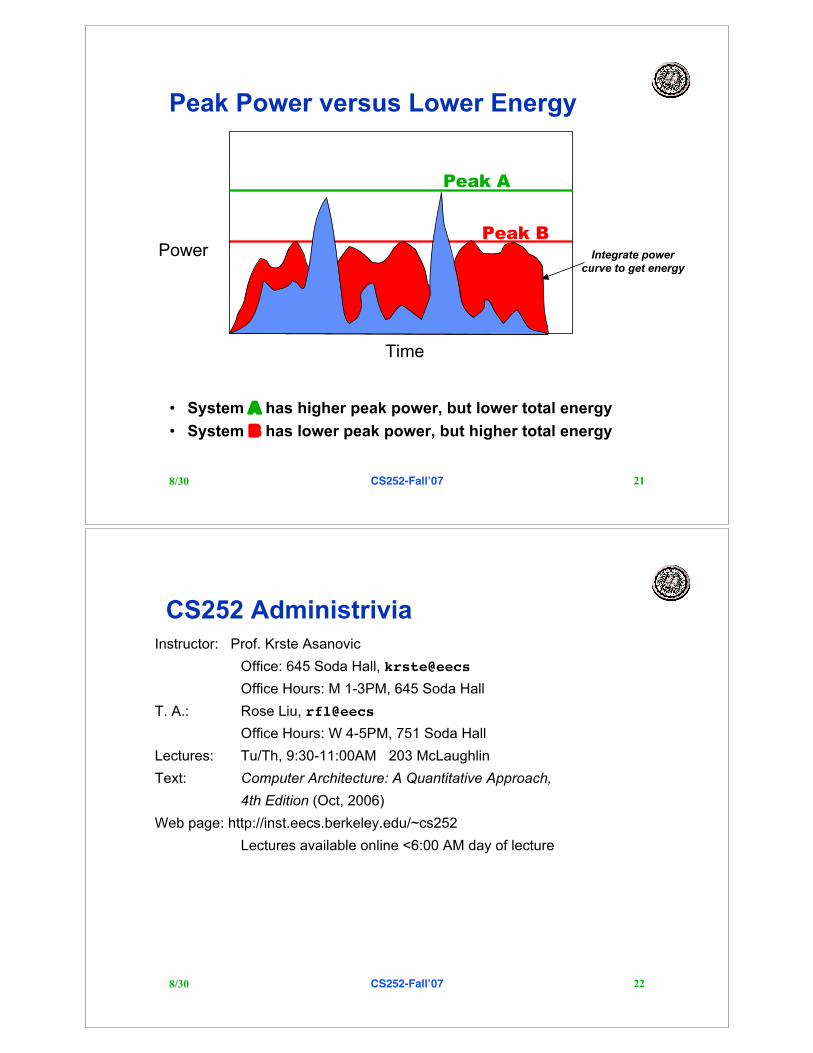
Peak Power versus Lower Energy
• System A has higher peak power, but lower total energy
• System B has lower peak power, but higher total energy
Power
Time
Peak A
Peak B
Integrate power
curve to get energy
8/30 CS252-Fall!07 22
CS252 Administrivia
Instructor: Prof. Krste Asanovic
Office: 645 Soda Hall, krste@eecs
Office Hours: M 1-3PM, 645 Soda Hall
T. A.: Rose Liu, rfl@eecs
Office Hours: W 4-5PM, 751 Soda Hall
Lectures: Tu/Th, 9:30-11:00AM 203 McLaughlin
Text: Computer Architecture: A Quantitative Approach,
4th Edition (Oct, 2006)
Web page: http://inst.eecs.berkeley.edu/~cs252
Lectures available online <6:00 AM day of lecture
8/30 CS252-Fall!07 23
CS252 Updates
• Prereq quiz will cover:– Finite state machines
– ISA designs & MIPS assembly code programming (today’s lecture)
– Simple pipelining (single-issue, in-order, today’s lecture)
– Simple caches (Tuesday’s lecture)
• Will try using Bspace this term to manage courseprivate material (readings, assignments)– https://bspace.berkeley.edu/portal
• Book order late at book store, will try and get youtemporary copies of text
8/30 CS252-Fall!07 24
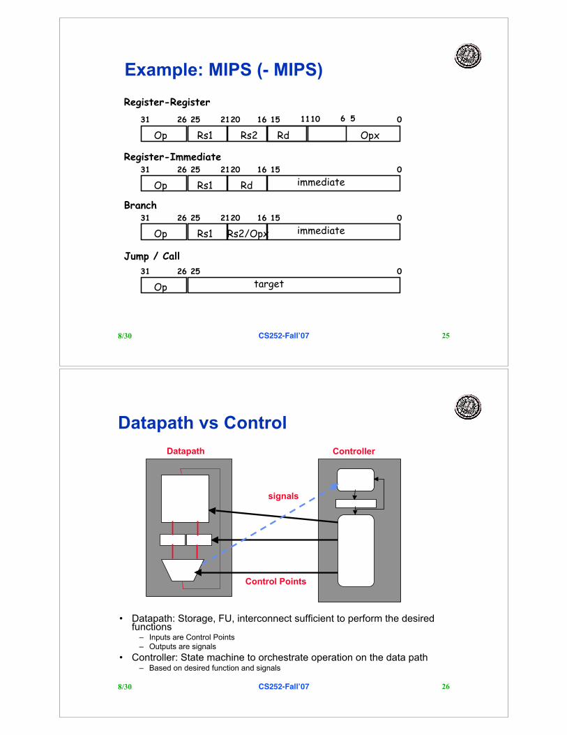
A "Typical" RISC ISA
• 32-bit fixed format instruction (3 formats)
• 32 32-bit GPR (R0 contains zero, DP take pair)
• 3-address, reg-reg arithmetic instruction
• Single address mode for load/store:base + displacement
– no indirection
• Simple branch conditions
• Delayed branch
see: SPARC, MIPS, HP PA-Risc, DEC Alpha, IBM PowerPC, CDC 6600, CDC 7600, Cray-1, Cray-2, Cray-3
8/30 CS252-Fall!07 25
Example: MIPS (- MIPS)
Op
31 26 01516202125
Rs1 Rd immediate
Op
31 26 025
Op
31 26 01516202125
Rs1 Rs2
target
Rd Opx
Register-Register
561011
Register-Immediate
Op
31 26 01516202125
Rs1 Rs2/Opx immediate
Branch
Jump / Call
8/30 CS252-Fall!07 26
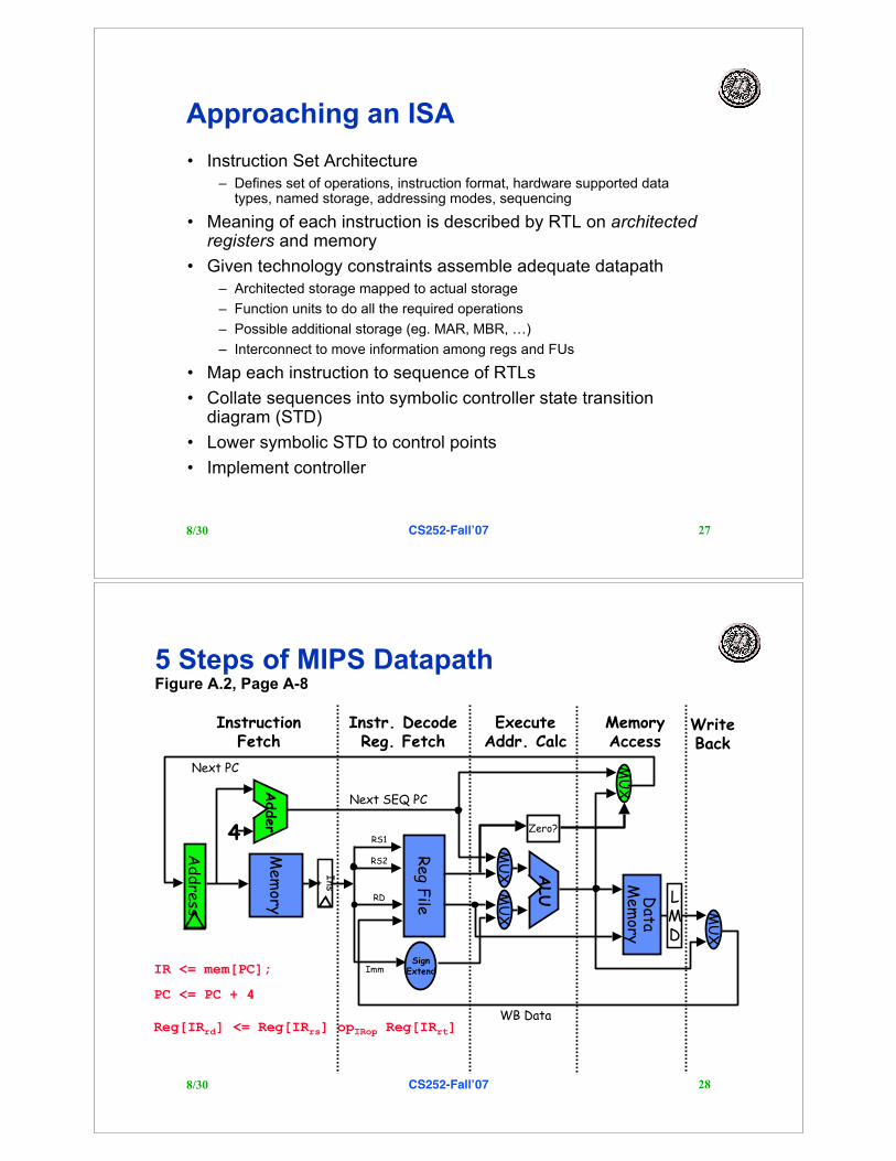
Datapath vs Control
• Datapath: Storage, FU, interconnect sufficient to perform the desiredfunctions
– Inputs are Control Points– Outputs are signals
• Controller: State machine to orchestrate operation on the data path– Based on desired function and signals
Datapath Controller
Control Points
signals
8/30 CS252-Fall!07 27
Approaching an ISA
• Instruction Set Architecture– Defines set of operations, instruction format, hardware supported data
types, named storage, addressing modes, sequencing
• Meaning of each instruction is described by RTL on architectedregisters and memory
• Given technology constraints assemble adequate datapath– Architected storage mapped to actual storage
– Function units to do all the required operations
– Possible additional storage (eg. MAR, MBR, …)
– Interconnect to move information among regs and FUs
• Map each instruction to sequence of RTLs
• Collate sequences into symbolic controller state transitiondiagram (STD)
• Lower symbolic STD to control points
• Implement controller
8/30 CS252-Fall!07 28
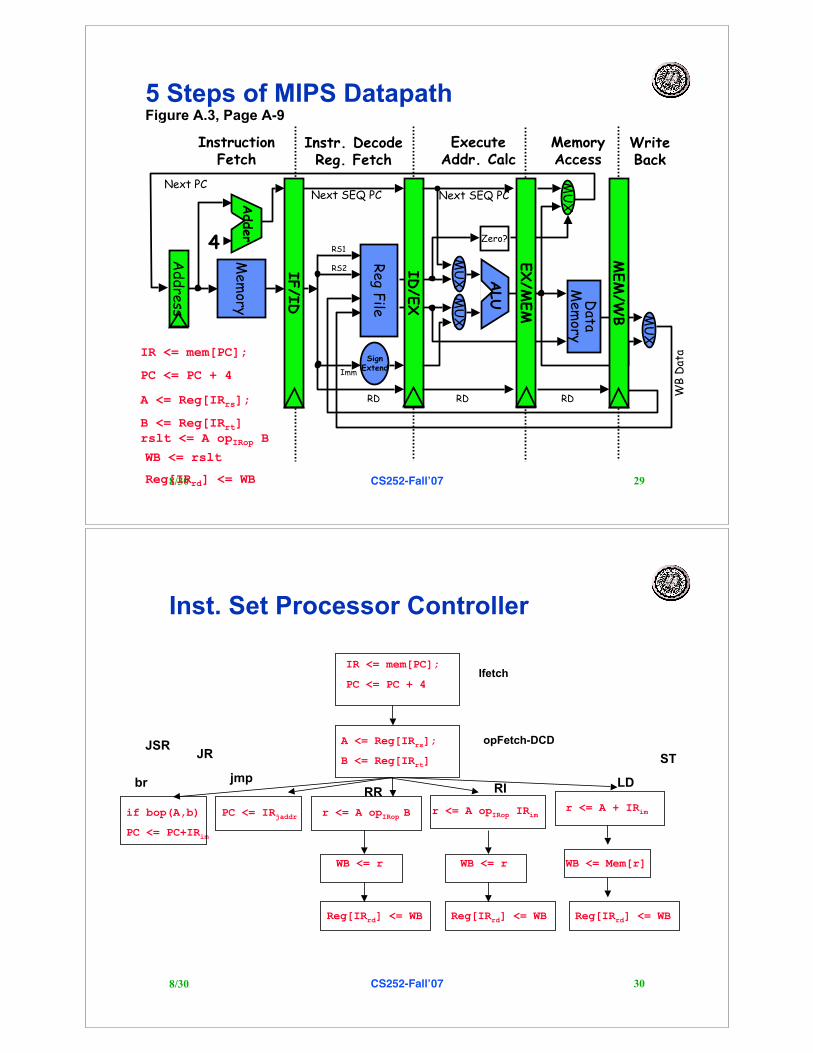
5 Steps of MIPS DatapathFigure A.2, Page A-8
MemoryAccess
WriteBack
InstructionFetch
Instr. DecodeReg. Fetch
ExecuteAddr. Calc
LMD
ALU
MU
X
Mem
ory
Reg F
ile
MU
XM
UX
Data
Mem
ory
MU
X
SignExtend
4
Adder Zero?
Next SEQ PC
Addre
ss
Next PC
WB Data
Inst
RD
RS1
RS2
ImmIR <= mem[PC];
PC <= PC + 4
Reg[IRrd] <= Reg[IRrs] opIRop Reg[IRrt]
8/30 CS252-Fall!07 29
5 Steps of MIPS DatapathFigure A.3, Page A-9
MemoryAccess
WriteBack
InstructionFetch
Instr. DecodeReg. Fetch
ExecuteAddr. Calc
ALU
Mem
ory
Reg F
ile
MU
XM
UX
Data
Mem
ory
MU
X
SignExtend
Zero?
IF/I
D
ID/E
X
MEM
/WB
EX/M
EM
4
Adder
Next SEQ PC Next SEQ PC
RD RD RD
WB
Dat
a
Next PC
Addre
ss
RS1
RS2
Imm
MU
X
IR <= mem[PC];
PC <= PC + 4
A <= Reg[IRrs];
B <= Reg[IRrt]
rslt <= A opIRop B
Reg[IRrd] <= WB
WB <= rslt
8/30 CS252-Fall!07 30
Inst. Set Processor Controller
IR <= mem[PC];
PC <= PC + 4
A <= Reg[IRrs];
B <= Reg[IRrt]
r <= A opIRop
B
Reg[IRrd] <= WB
WB <= r
Ifetch
opFetch-DCD
PC <= IRjaddr
if bop(A,b)
PC <= PC+IRim
br jmpRR
r <= A opIRop
IRim
Reg[IRrd] <= WB
WB <= r
RI
r <= A + IRim
WB <= Mem[r]
Reg[IRrd] <= WB
LD
STJSR
JR
8/30 CS252-Fall!07 31
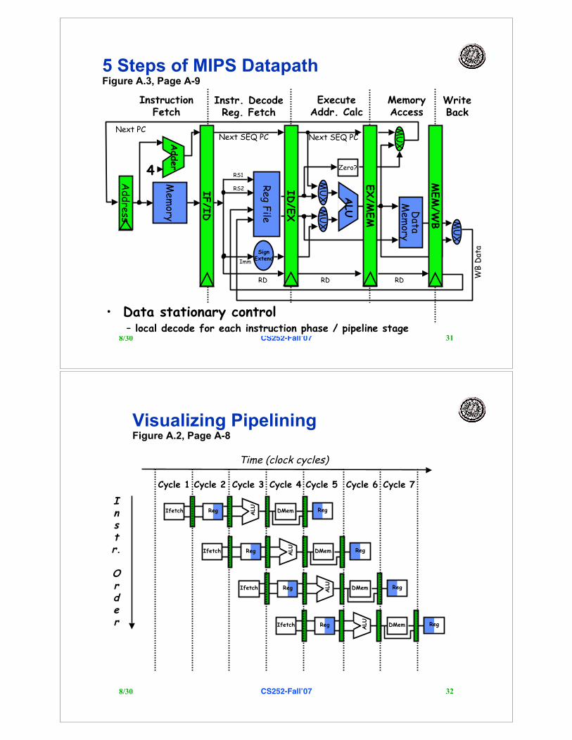
5 Steps of MIPS DatapathFigure A.3, Page A-9
MemoryAccess
WriteBack
InstructionFetch
Instr. DecodeReg. Fetch
ExecuteAddr. Calc
ALU
Mem
ory
Reg F
ile
MU
XM
UX
Data
Mem
ory
MU
X
SignExtend
Zero?
IF/I
D
ID/E
X
MEM
/WB
EX/M
EM
4
Adder
Next SEQ PC Next SEQ PC
RD RD RD
WB
Dat
a
• Data stationary control– local decode for each instruction phase / pipeline stage
Next PC
Addre
ss
RS1
RS2
Imm
MU
X
8/30 CS252-Fall!07 32
Visualizing PipeliningFigure A.2, Page A-8
Instr.
Order
Time (clock cycles)
Reg
ALU
DMemIfetch Reg
Reg ALU
DMemIfetch Reg
Reg ALU
DMemIfetch Reg
Reg
ALU
DMemIfetch Reg
Cycle 1 Cycle 2 Cycle 3 Cycle 4 Cycle 6 Cycle 7Cycle 5
8/30 CS252-Fall!07 33
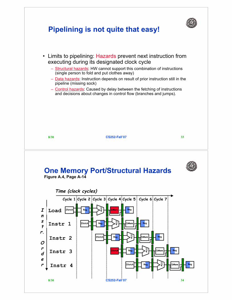
Pipelining is not quite that easy!
• Limits to pipelining: Hazards prevent next instruction fromexecuting during its designated clock cycle
– Structural hazards: HW cannot support this combination of instructions(single person to fold and put clothes away)
– Data hazards: Instruction depends on result of prior instruction still in thepipeline (missing sock)
– Control hazards: Caused by delay between the fetching of instructionsand decisions about changes in control flow (branches and jumps).
8/30 CS252-Fall!07 34
One Memory Port/Structural HazardsFigure A.4, Page A-14
Instr.
Order
Time (clock cycles)
Load
Instr 1
Instr 2
Instr 3
Instr 4
Reg
ALU
DMemIfetch Reg
Reg ALU
DMemIfetch Reg
Reg ALU
DMemIfetch Reg
Reg
ALU
DMemIfetch Reg
Cycle 1 Cycle 2 Cycle 3 Cycle 4 Cycle 6 Cycle 7Cycle 5
Reg
ALU
DMemIfetch Reg
8/30 CS252-Fall!07 35
One Memory Port/Structural Hazards(Similar to Figure A.5, Page A-15)
Instr.
Order
Time (clock cycles)
Load
Instr 1
Instr 2
Stall
Instr 3
Reg
ALU
DMemIfetch Reg
Reg
ALU
DMemIfetch Reg
Reg
ALU
DMemIfetch Reg
Cycle 1 Cycle 2 Cycle 3 Cycle 4 Cycle 6 Cycle 7Cycle 5
Reg
ALU
DMemIfetch Reg
Bubble Bubble Bubble BubbleBubble
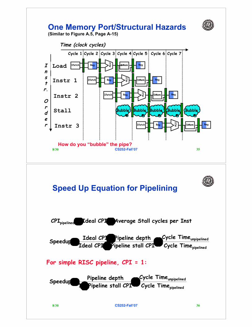
How do you “bubble” the pipe?
8/30 CS252-Fall!07 36
Speed Up Equation for Pipelining
pipelined
dunpipeline
TimeCycle
TimeCycle
CPI stall Pipeline CPI Ideal
depth Pipeline CPI Ideal Speedup !
+
!=
pipelined
dunpipeline
TimeCycle
TimeCycle
CPI stall Pipeline 1
depth Pipeline Speedup !
+=
Instper cycles Stall Average CPI Ideal CPIpipelined +=
For simple RISC pipeline, CPI = 1:
8/30 CS252-Fall!07 37
Example: Dual-port vs. Single-port
• Machine A: Dual ported memory (“Harvard Architecture”)
• Machine B: Single ported memory, but its pipelined implementation has a1.05 times faster clock rate
• Ideal CPI = 1 for both
• Loads are 40% of instructions executed
SpeedUpA = Pipeline Depth/(1 + 0) x (clockunpipe/clockpipe)
= Pipeline Depth
SpeedUpB = Pipeline Depth/(1 + 0.4 x 1) x (clockunpipe/(clockunpipe / 1.05)
= (Pipeline Depth/1.4) x 1.05
= 0.75 x Pipeline Depth
SpeedUpA / SpeedUpB = Pipeline Depth/(0.75 x Pipeline Depth) = 1.33
• Machine A is 1.33 times faster
8/30 CS252-Fall!07 38
Instr.
Order
add r1,r2,r3
sub r4,r1,r3
and r6,r1,r7
or r8,r1,r9
xor r10,r1,r11
Reg
ALU
DMemIfetch Reg
Reg
ALU
DMemIfetch Reg
Reg
ALU
DMemIfetch Reg
Reg
ALU
DMemIfetch Reg
Reg
ALU
DMemIfetch Reg
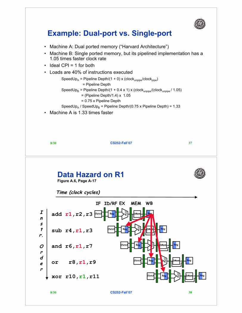
Data Hazard on R1Figure A.6, Page A-17
Time (clock cycles)
IF ID/RF EX MEM WB
8/30 CS252-Fall!07 39
• Read After Write (RAW)InstrJ tries to read operand before InstrI writes it
• Caused by a “Dependence” (in compiler nomenclature).This hazard results from an actual need for communication.
Three Generic Data Hazards
I: add r1,r2,r3
J: sub r4,r1,r3
8/30 CS252-Fall!07 40
• Write After Read (WAR)InstrJ writes operand before InstrI reads it
• Called an “anti-dependence” by compiler writers.This results from reuse of the name “r1”.
• Can’t happen in MIPS 5 stage pipeline because:
– All instructions take 5 stages, and
– Reads are always in stage 2, and
– Writes are always in stage 5
I: sub r4,r1,r3
J: add r1,r2,r3
K: mul r6,r1,r7
Three Generic Data Hazards
8/30 CS252-Fall!07 41
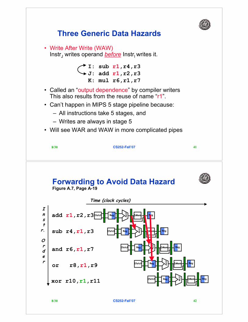
Three Generic Data Hazards
• Write After Write (WAW)InstrJ writes operand before InstrI writes it.
• Called an “output dependence” by compiler writersThis also results from the reuse of name “r1”.
• Can’t happen in MIPS 5 stage pipeline because:
– All instructions take 5 stages, and
– Writes are always in stage 5
• Will see WAR and WAW in more complicated pipes
I: sub r1,r4,r3
J: add r1,r2,r3
K: mul r6,r1,r7
8/30 CS252-Fall!07 42
Time (clock cycles)
Forwarding to Avoid Data HazardFigure A.7, Page A-19
Instr.
Order
add r1,r2,r3
sub r4,r1,r3
and r6,r1,r7
or r8,r1,r9
xor r10,r1,r11
Reg
ALU
DMemIfetch Reg
Reg
ALU
DMemIfetch Reg
Reg
ALU
DMemIfetch Reg
Reg
ALU
DMemIfetch Reg
Reg
ALU
DMemIfetch Reg
8/30 CS252-Fall!07 43
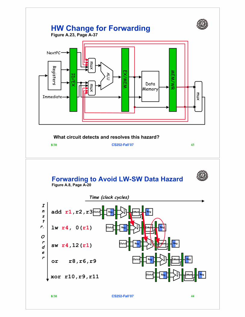
HW Change for ForwardingFigure A.23, Page A-37
ME
M/W
R
ID
/EX
EX
/ME
M
DataMemory
ALU
mux
mux
Registe
rs
NextPC
Immediate
mux
What circuit detects and resolves this hazard?
8/30 CS252-Fall!07 44
Time (clock cycles)
Forwarding to Avoid LW-SW Data HazardFigure A.8, Page A-20
Instr.
Order
add r1,r2,r3
lw r4, 0(r1)
sw r4,12(r1)
or r8,r6,r9
xor r10,r9,r11
Reg
ALU
DMemIfetch Reg
Reg
ALU
DMemIfetch Reg
Reg
ALU
DMemIfetch Reg
Reg
ALU
DMemIfetch Reg
Reg
ALU
DMemIfetch Reg
8/30 CS252-Fall!07 45
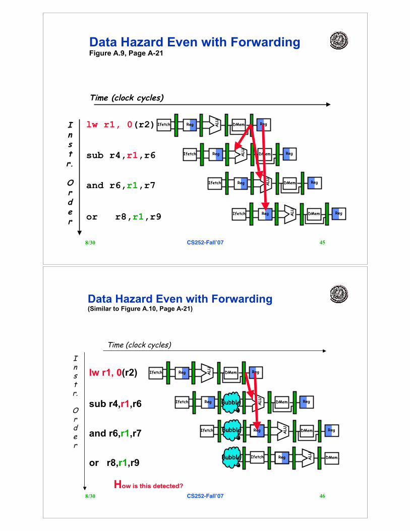
Time (clock cycles)
Instr.
Order
lw r1, 0(r2)
sub r4,r1,r6
and r6,r1,r7
or r8,r1,r9
Data Hazard Even with ForwardingFigure A.9, Page A-21
Reg ALU
DMemIfetch Reg
Reg ALU
DMemIfetch Reg
Reg ALU
DMemIfetch Reg
Reg ALU
DMemIfetch Reg
8/30 CS252-Fall!07 46
Data Hazard Even with Forwarding(Similar to Figure A.10, Page A-21)
Time (clock cycles)
or r8,r1,r9
Instr.
Order
lw r1, 0(r2)
sub r4,r1,r6
and r6,r1,r7
Reg ALU
DMemIfetch Reg
RegIfetch
ALU
DMem RegBubble
Ifetch
ALU
DMem RegBubble Reg
Ifetch ALU
DMemBubble Reg
How is this detected?
8/30 CS252-Fall!07 47
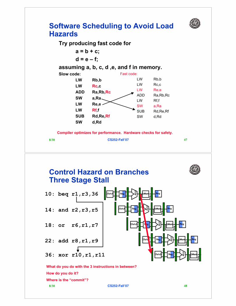
Try producing fast code for
a = b + c;
d = e – f;
assuming a, b, c, d ,e, and f in memory.Slow code:
LW Rb,b
LW Rc,c
ADD Ra,Rb,Rc
SW a,Ra
LW Re,e
LW Rf,f
SUB Rd,Re,Rf
SW d,Rd
Software Scheduling to Avoid LoadHazards
Fast code:
LW Rb,b
LW Rc,c
LW Re,e
ADD Ra,Rb,Rc
LW Rf,f
SW a,Ra
SUB Rd,Re,Rf
SW d,Rd
Compiler optimizes for performance. Hardware checks for safety.
8/30 CS252-Fall!07 48
Control Hazard on BranchesThree Stage Stall
10: beq r1,r3,36
14: and r2,r3,r5
18: or r6,r1,r7
22: add r8,r1,r9
36: xor r10,r1,r11
Reg ALU
DMemIfetch Reg
Reg ALU
DMemIfetch Reg
Reg ALU
DMemIfetch Reg
Reg
ALU
DMemIfetch Reg
Reg
ALU
DMemIfetch Reg
What do you do with the 3 instructions in between?
How do you do it?
Where is the “commit”?
8/30 CS252-Fall!07 49
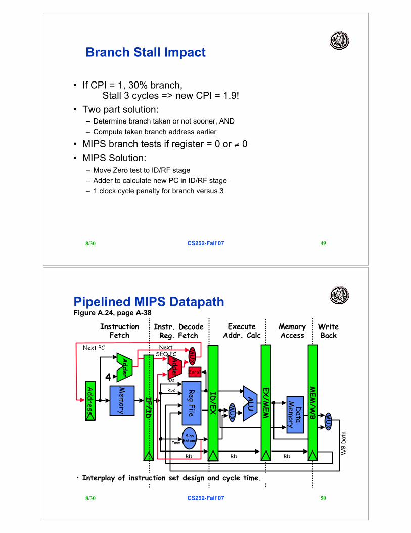
Branch Stall Impact
• If CPI = 1, 30% branch,Stall 3 cycles => new CPI = 1.9!
• Two part solution:– Determine branch taken or not sooner, AND
– Compute taken branch address earlier
• MIPS branch tests if register = 0 or $ 0
• MIPS Solution:– Move Zero test to ID/RF stage
– Adder to calculate new PC in ID/RF stage
– 1 clock cycle penalty for branch versus 3
8/30 CS252-Fall!07 50
Adder
IF/I
D
Pipelined MIPS DatapathFigure A.24, page A-38
MemoryAccess
WriteBack
InstructionFetch
Instr. DecodeReg. Fetch
ExecuteAddr. Calc
ALU
Mem
ory
Reg F
ile
MU
X
Data
Mem
ory
MU
X
SignExtend
Zero?
MEM
/WB
EX/M
EM
4
Adder
NextSEQ PC
RD RD RD
WB
Dat
a
• Interplay of instruction set design and cycle time.
Next PC
Addre
ss
RS1
RS2
Imm
MU
X
ID/E
X
8/30 CS252-Fall!07 51
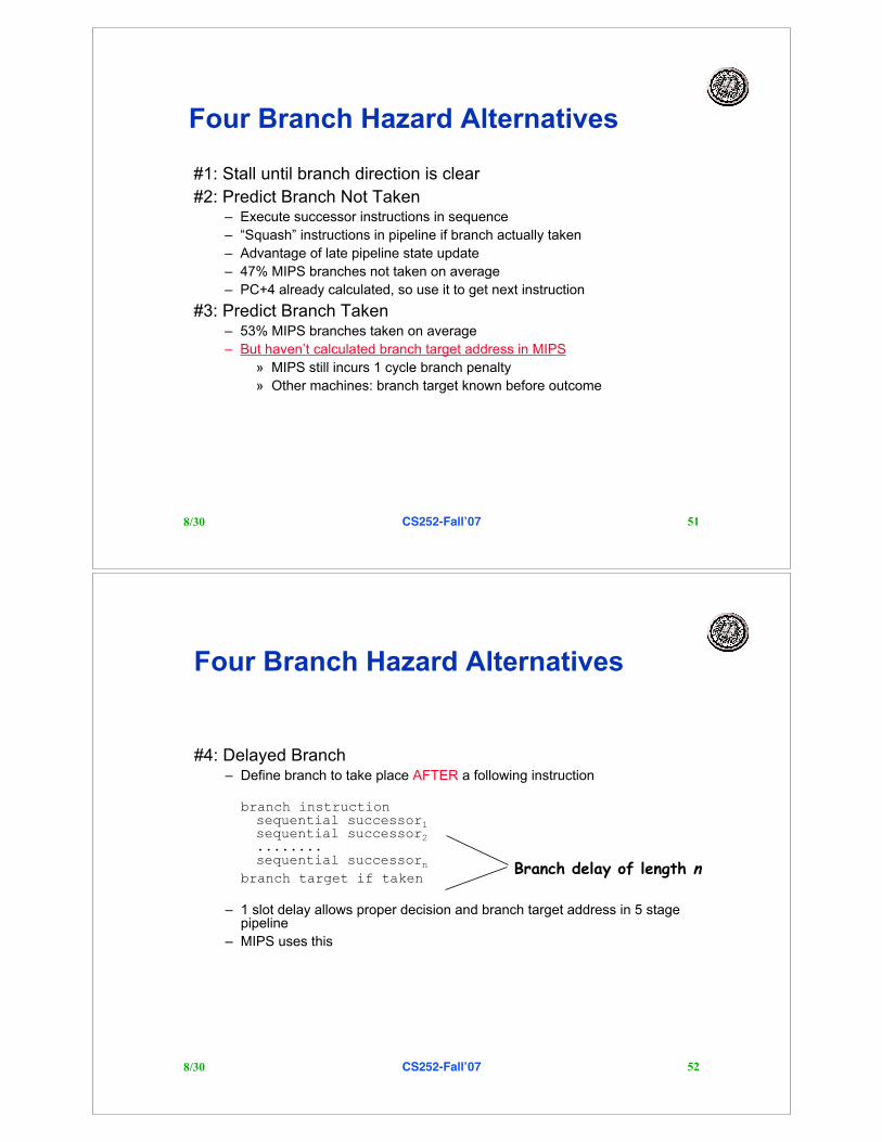
Four Branch Hazard Alternatives
#1: Stall until branch direction is clear
#2: Predict Branch Not Taken– Execute successor instructions in sequence
– “Squash” instructions in pipeline if branch actually taken
– Advantage of late pipeline state update
– 47% MIPS branches not taken on average
– PC+4 already calculated, so use it to get next instruction
#3: Predict Branch Taken– 53% MIPS branches taken on average
– But haven’t calculated branch target address in MIPS
» MIPS still incurs 1 cycle branch penalty
» Other machines: branch target known before outcome
8/30 CS252-Fall!07 52
Four Branch Hazard Alternatives
#4: Delayed Branch– Define branch to take place AFTER a following instruction
branch instructionsequential successor1sequential successor2........sequential successorn
branch target if taken
– 1 slot delay allows proper decision and branch target address in 5 stagepipeline
– MIPS uses this
Branch delay of length n
8/30 CS252-Fall!07 53
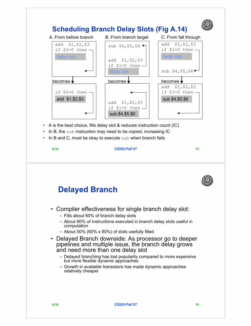
Scheduling Branch Delay Slots (Fig A.14)
• A is the best choice, fills delay slot & reduces instruction count (IC)
• In B, the sub instruction may need to be copied, increasing IC
• In B and C, must be okay to execute sub when branch fails
add $1,$2,$3
if $2=0 then
delay slot
A. From before branch B. From branch target C. From fall through
add $1,$2,$3
if $1=0 then
delay slot
add $1,$2,$3
if $1=0 then
delay slot
sub $4,$5,$6
sub $4,$5,$6
becomes becomes becomes
if $2=0 then
add $1,$2,$3add $1,$2,$3
if $1=0 then
sub $4,$5,$6
add $1,$2,$3
if $1=0 then
sub $4,$5,$6
8/30 CS252-Fall!07 54
Delayed Branch
• Compiler effectiveness for single branch delay slot:– Fills about 60% of branch delay slots
– About 80% of instructions executed in branch delay slots useful incomputation
– About 50% (60% x 80%) of slots usefully filled
• Delayed Branch downside: As processor go to deeperpipelines and multiple issue, the branch delay growsand need more than one delay slot
– Delayed branching has lost popularity compared to more expensivebut more flexible dynamic approaches
– Growth in available transistors has made dynamic approachesrelatively cheaper
8/30 CS252-Fall!07 55
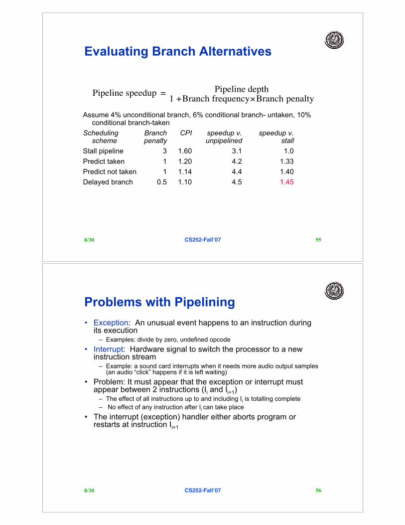
Evaluating Branch Alternatives
Assume 4% unconditional branch, 6% conditional branch- untaken, 10%conditional branch-taken
Scheduling Branch CPI speedup v. speedup v.scheme penalty unpipelined stall
Stall pipeline 3 1.60 3.1 1.0
Predict taken 1 1.20 4.2 1.33
Predict not taken 1 1.14 4.4 1.40
Delayed branch 0.5 1.10 4.5 1.45
Pipeline speedup = Pipeline depth1 +Branch frequency!Branch penalty
8/30 CS252-Fall!07 56
Problems with Pipelining
• Exception: An unusual event happens to an instruction duringits execution
– Examples: divide by zero, undefined opcode
• Interrupt: Hardware signal to switch the processor to a newinstruction stream
– Example: a sound card interrupts when it needs more audio output samples(an audio “click” happens if it is left waiting)
• Problem: It must appear that the exception or interrupt mustappear between 2 instructions (Ii and Ii+1)
– The effect of all instructions up to and including Ii is totalling complete
– No effect of any instruction after Ii can take place
• The interrupt (exception) handler either aborts program orrestarts at instruction Ii+1
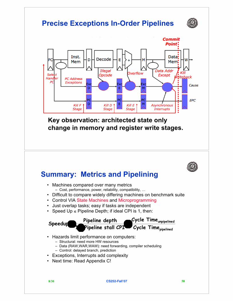
Precise Exceptions In-Order Pipelines
Key observation: architected state only
change in memory and register write stages.
8/30 CS252-Fall!07 58
Summary: Metrics and Pipelining
• Machines compared over many metrics– Cost, performance, power, reliability, compatibility, …
• Difficult to compare widely differing machines on benchmark suite• Control VIA State Machines and Microprogramming• Just overlap tasks; easy if tasks are independent• Speed Up % Pipeline Depth; if ideal CPI is 1, then:
• Hazards limit performance on computers:– Structural: need more HW resources– Data (RAW,WAR,WAW): need forwarding, compiler scheduling– Control: delayed branch, prediction
• Exceptions, Interrupts add complexity• Next time: Read Appendix C!
pipelined
dunpipeline
TimeCycle
TimeCycle
CPI stall Pipeline 1
depth Pipeline Speedup !
+=


![[Architecture ebook] buddhist architecture](https://img.pdfslide.net/doc/110x75/54966961b47959ec108b48c6/architecture-ebook-buddhist-architecture.jpg)