CS 361 – Chapter 4

• Improvements to BST– Why?– AVL tree (today)

• Skills: insert & delete

– Red-black tree– Splay tree

• Non-binary tree implementation• Non-tree implementation

AVL trees

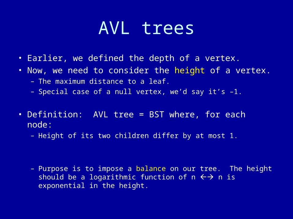
• Earlier, we defined the depth of a vertex.• Now, we need to consider the height of a vertex.

– The maximum distance to a leaf.– Special case of a null vertex, we’d say it’s –1.

• Definition: AVL tree = BST where, for each node:– Height of its two children differ by at most 1.

– Purpose is to impose a balance on our tree. The height should be a logarithmic function of n n is exponential in the height.

Height vs. size

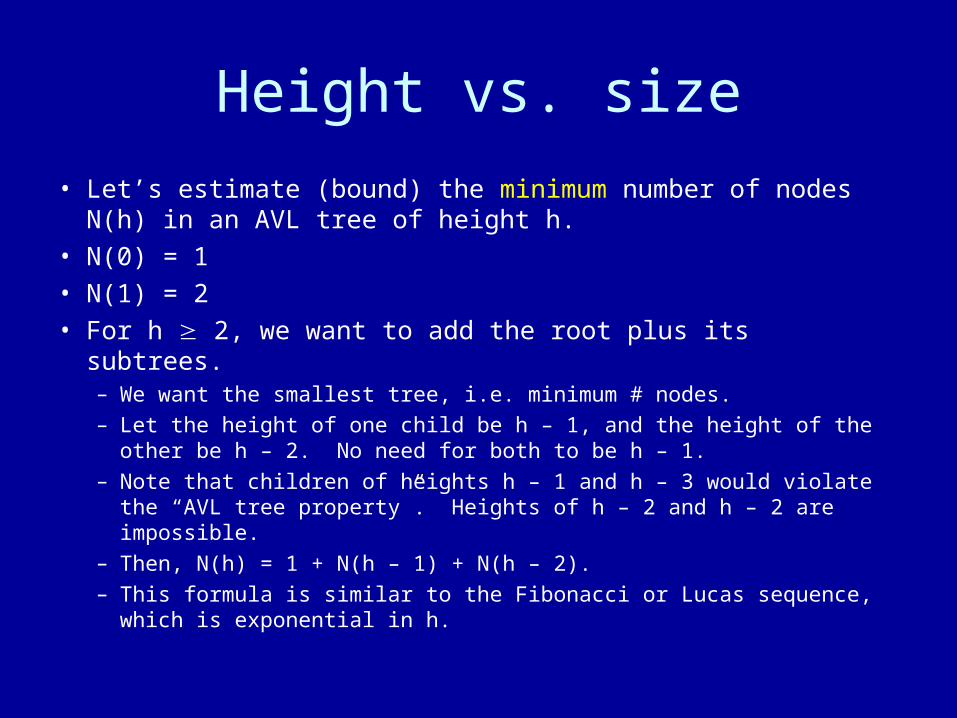
• Let’s estimate (bound) the minimum number of nodes N(h) in an AVL tree of height h.

• N(0) = 1• N(1) = 2• For h 2, we want to add the root plus its subtrees.

– We want the smallest tree, i.e. minimum # nodes.

– Let the height of one child be h – 1, and the height of the other be h – 2. No need for both to be h – 1.

– Note that children of heights h – 1 and h – 3 would violate the “AVL tree property”. Heights of h – 2 and h – 2 are impossible.

– Then, N(h) = 1 + N(h – 1) + N(h – 2).

– This formula is similar to the Fibonacci or Lucas sequence, which is exponential in h.

AVL Insertion

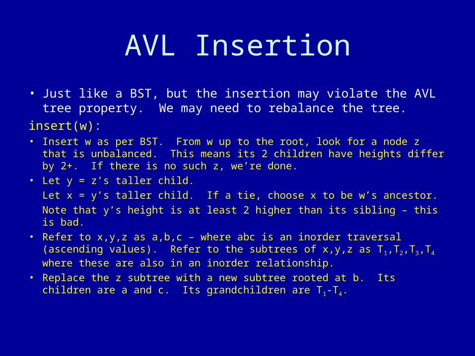
• Just like a BST, but the insertion may violate the AVL tree property. We may need to rebalance the tree.

insert(w):• Insert w as per BST. From w up to the root, look for a node z that is

unbalanced. This means its 2 children have heights differ by 2+. If there is no such z, we’re done.

• Let y = z’s taller child.

Let x = y’s taller child. If a tie, choose x to be w’s ancestor.

Note that y’s height is at least 2 higher than its sibling – this is bad.• Refer to x,y,z as a,b,c – where abc is an inorder traversal (ascending

values). Refer to the subtrees of x,y,z as T1,T2,T3,T4 where these are also in an inorder relationship.

• Replace the z subtree with a new subtree rooted at b. Its children are a and c. Its grandchildren are T1-T4.

Insert examples

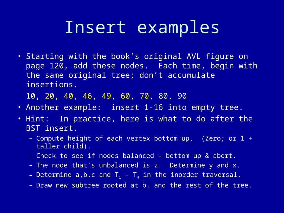
• Starting with the book’s original AVL figure on page 120, add these nodes. Each time, begin with the same original tree; don’t accumulate insertions.

10, 20, 40, 46, 49, 60, 70, 80, 90• Another example: insert 1-16 into empty tree.• Hint: In practice, here is what to do after the BST insert.

– Compute height of each vertex bottom up. (Zero; or 1 + taller child).

– Check to see if nodes balanced – bottom up & abort.– The node that’s unbalanced is z. Determine y and x.

– Determine a,b,c and T1 – T4 in the inorder traversal.

– Draw new subtree rooted at b, and the rest of the tree.

Deletion

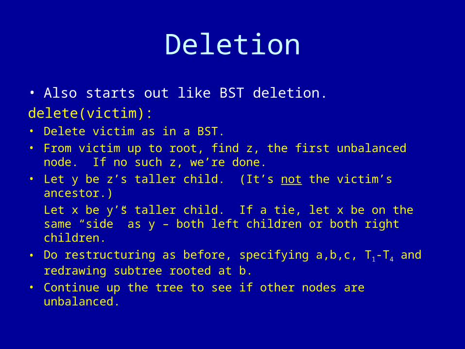
• Also starts out like BST deletion.

delete(victim):• Delete victim as in a BST.• From victim up to root, find z, the first unbalanced node. If no such

z, we’re done.• Let y be z’s taller child. (It’s not the victim’s ancestor.)

Let x be y’s taller child. If a tie, let x be on the same “side” as y – both left children or both right children.

• Do restructuring as before, specifying a,b,c, T1-T4 and redrawing subtree rooted at b.

• Continue up the tree to see if other nodes are unbalanced.

Deletion examples

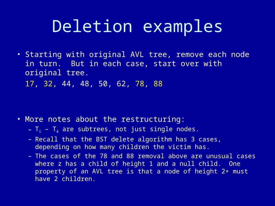
• Starting with original AVL tree, remove each node in turn. But in each case, start over with original tree.

17, 32, 44, 48, 50, 62, 78, 88

• More notes about the restructuring:– T1 – T4 are subtrees, not just single nodes.

– Recall that the BST delete algorithm has 3 cases, depending on how many children the victim has.

– The cases of the 78 and 88 removal above are unusual cases where z has a child of height 1 and a null child. One property of an AVL tree is that a node of height 2+ must have 2 children.

B trees

• Also called: Multi-way search tree– properties– insert– delete

B trees

• Let’s generalize the binary search tree.• Instead of “binary”: “multi-way”

– Nodes may have > 2 children.

• They come in many sizes. Let’s look at the case of the (2,4) tree, which is a “B tree”.– B tree is a multi-way search tree where all nodes except the root

must have t to 2t children. The root needs 2+ children.

• Purpose: wider, shorter tree than the BST. Good for a huge amount of data where we want to reduce # of disk accesses (page faults).

Properties

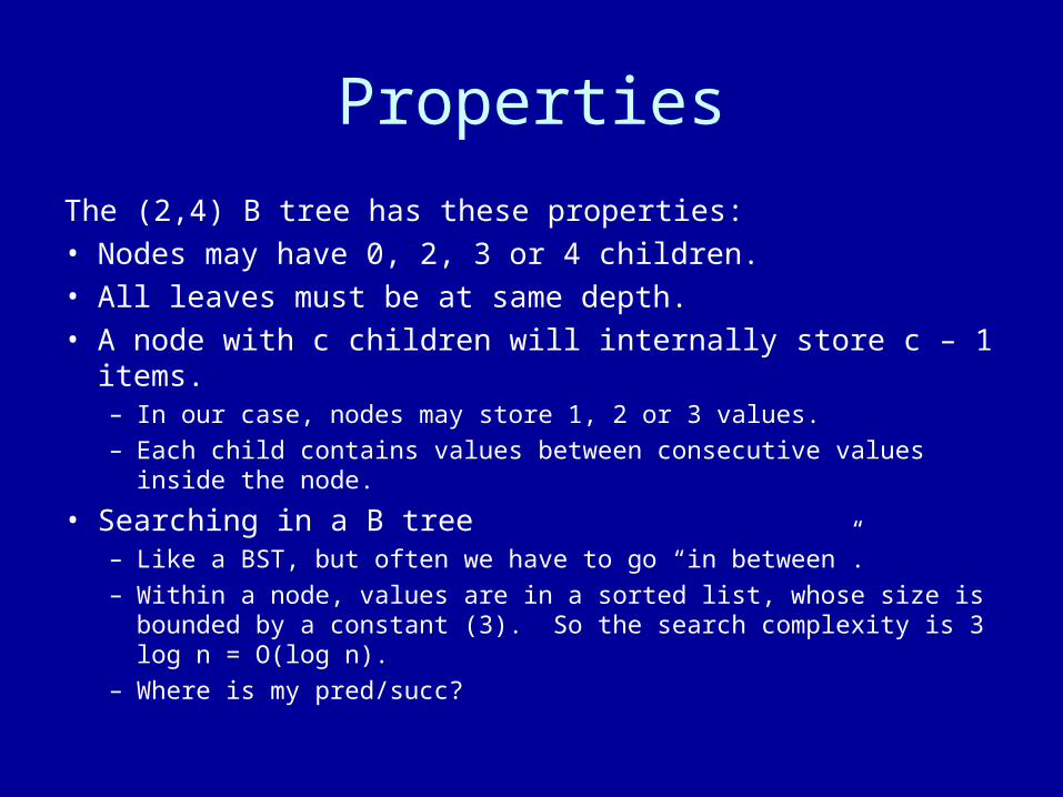
The (2,4) B tree has these properties:• Nodes may have 0, 2, 3 or 4 children.• All leaves must be at same depth.• A node with c children will internally store c – 1 items.

– In our case, nodes may store 1, 2 or 3 values.– Each child contains values between consecutive values inside the

node.

• Searching in a B tree– Like a BST, but often we have to go “in between”.– Within a node, values are in a sorted list, whose size is bounded

by a constant (3). So the search complexity is 3 log n = O(log n).

– Where is my pred/succ?

B tree Insertion

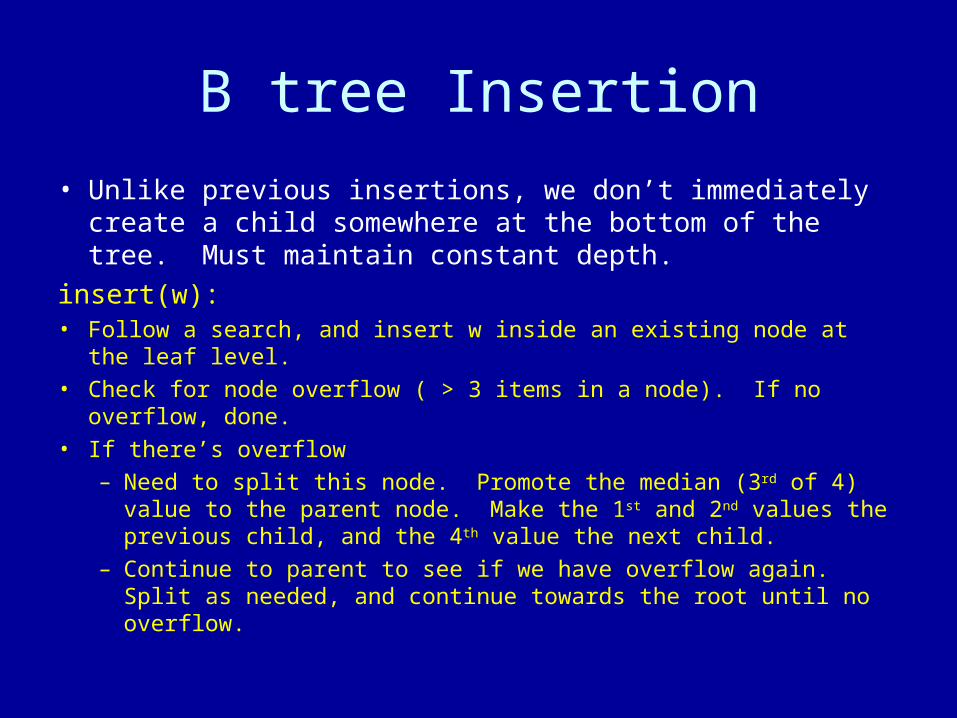
• Unlike previous insertions, we don’t immediately create a child somewhere at the bottom of the tree. Must maintain constant depth.

insert(w):• Follow a search, and insert w inside an existing node at the leaf

level.• Check for node overflow ( > 3 items in a node). If no overflow, done.• If there’s overflow

– Need to split this node. Promote the median (3rd of 4) value to the parent node. Make the 1st and 2nd values the previous child, and the 4th value the next child.

– Continue to parent to see if we have overflow again. Split as needed, and continue towards the root until no overflow.

Analysis & examples

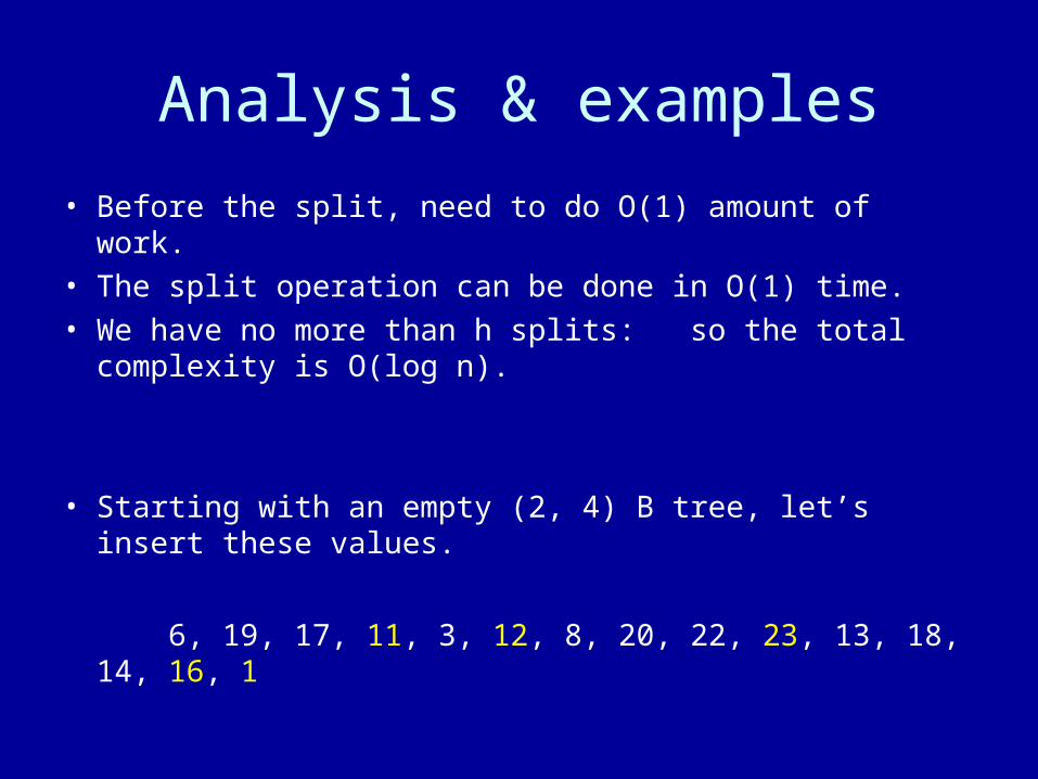
• Before the split, need to do O(1) amount of work.• The split operation can be done in O(1) time.• We have no more than h splits: so the total complexity

is O(log n).

• Starting with an empty (2, 4) B tree, let’s insert these values.

6, 19, 17, 11, 3, 12, 8, 20, 22, 23, 13, 18, 14, 16, 1

Deletion

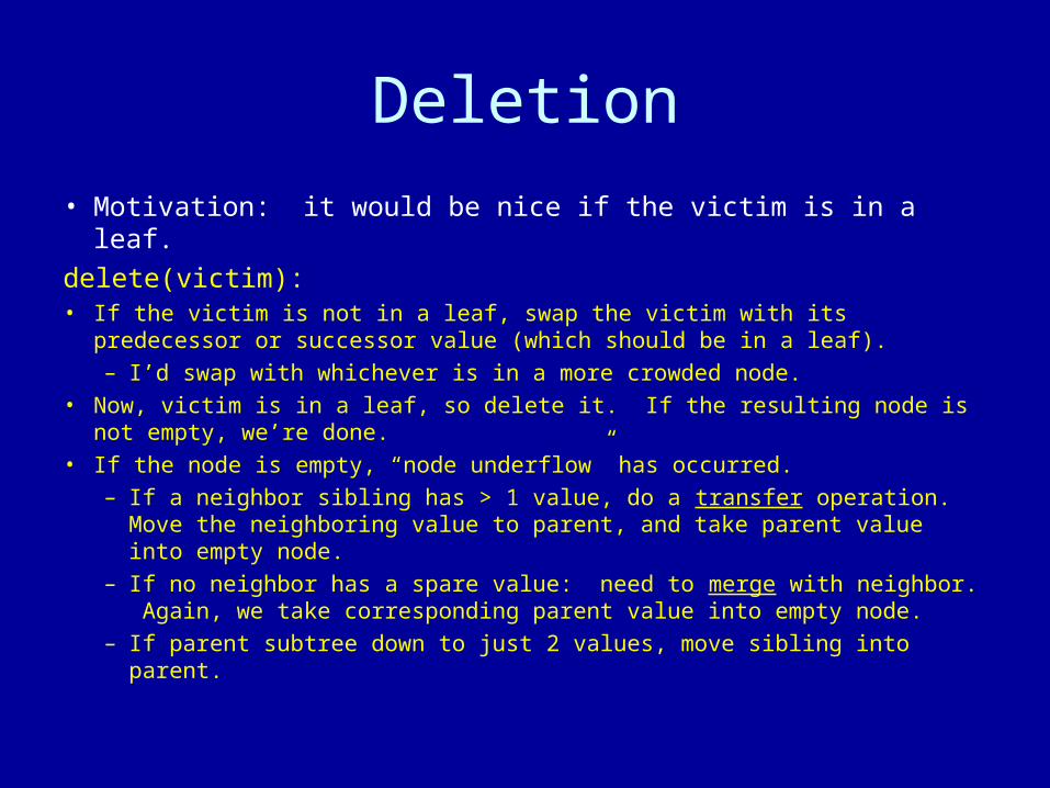
• Motivation: it would be nice if the victim is in a leaf.

delete(victim):• If the victim is not in a leaf, swap the victim with its predecessor or

successor value (which should be in a leaf).– I’d swap with whichever is in a more crowded node.

• Now, victim is in a leaf, so delete it. If the resulting node is not empty, we’re done.

• If the node is empty, “node underflow” has occurred.– If a neighbor sibling has > 1 value, do a transfer operation. Move the

neighboring value to parent, and take parent value into empty node.– If no neighbor has a spare value: need to merge with neighbor.

Again, we take corresponding parent value into empty node.– If parent subtree down to just 2 values, move sibling into parent.

Deletion: transfer

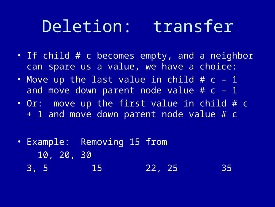
• If child # c becomes empty, and a neighbor can spare us a value, we have a choice:

• Move up the last value in child # c – 1 and move down parent node value # c – 1

• Or: move up the first value in child # c + 1 and move down parent node value # c

• Example: Removing 15 from

10, 20, 30

3, 5 15 22, 25 35

Deletion: merge

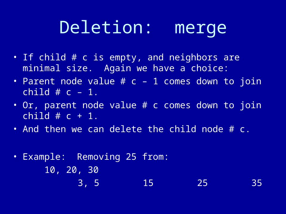
• If child # c is empty, and neighbors are minimal size. Again we have a choice:

• Parent node value # c – 1 comes down to join child # c – 1.• Or, parent node value # c comes down to join child # c + 1.• And then we can delete the child node # c.

• Example: Removing 25 from:

10, 20, 30

3, 5 15 25 35

Deletion examples

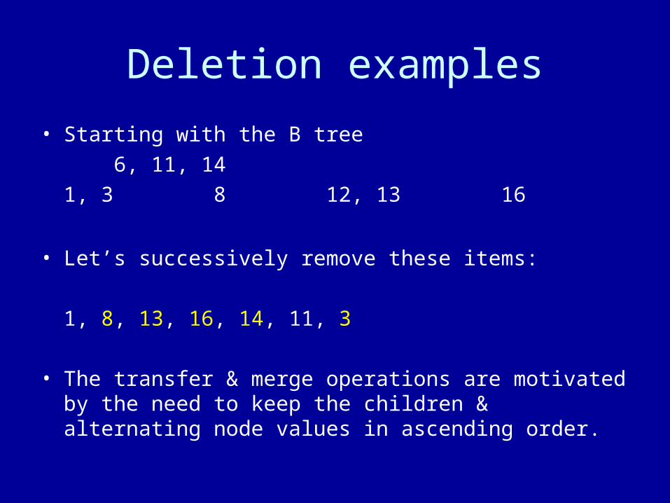
• Starting with the B tree

6, 11, 14

1, 3 8 12, 13 16

• Let’s successively remove these items:

1, 8, 13, 16, 14, 11, 3

• The transfer & merge operations are motivated by the need to keep the children & alternating node values in ascending order.

More on deletion

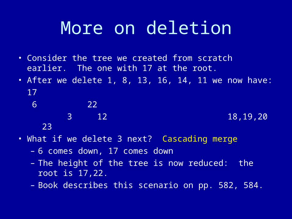
• Consider the tree we created from scratch earlier. The one with 17 at the root.

• After we delete 1, 8, 13, 16, 14, 11 we now have:

17

6 22

3 12 18,19,20 23• What if we delete 3 next? Cascading merge

– 6 comes down, 17 comes down– The height of the tree is now reduced: the root is

17,22.– Book describes this scenario on pp. 582, 584.

Red-black trees

• (Review B tree deletion if necessary)

• Red-black trees– A 2nd approach to balancing a BST– Analogous to the (2, 4) B tree

Red-black trees

Definition• Like the AVL tree, a red-black tree is a specialized form of

binary search tree.• At each node, we keep 1 more attribute: its color, which is

either red or black.– In addition to the usual attributes of key, item, left, right, parent

• Need to pay attention to null leaves– Logically consider them honorary nodes in the tree.– Why? Without them, properties of red-black tree could be satisfied by

very unbalanced tree– Simplifies the deletion algorithm

• In addition to being a BST, a red-black tree must satisfy additional properties at all times….

Properties

1. The root is black.

2. Null leaves are black.

3. Children of a red node are black.

4. All paths from root to a null leaf encounter the same number of black nodes. This is the black height of the tree.– Slightly different definitions of black height are possible.

• Important consequence:– A path from the root to a leaf cannot see 2 reds in a row. Combine

this fact with the black height… Therefore, no path is more than twice as long as any other. This is how we maintain balance.

B tree analogy

• In a (2, 4) B tree, internal nodes may have 2, 3 or 4 children. In other words they may have 1, 2 or 3 values per node.

• How to convert to red-black tree.– 1-value node: no real change– 2-value node: one value become parent of the other– 3-value node: middle value becomes parent of 1st and 3rd values– In all cases, the “parent” is black, and the former children of the

B tree node are also black.– The only red nodes are the secondary value in the 2-value node

and the 1st & 3rd values of the 3-value node.

Convert example

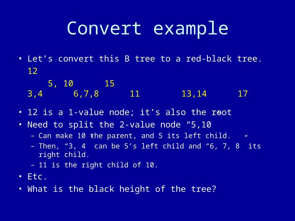
• Let’s convert this B tree to a red-black tree.

12

5, 10 153,4 6,7,8 11 13,14 17

• 12 is a 1-value node; it’s also the root

• Need to split the 2-value node “5,10”– Can make 10 the parent, and 5 its left child.

– Then, “3, 4” can be 5’s left child and “6, 7, 8” its right child.

– 11 is the right child of 10.

• Etc.

• What is the black height of the tree?

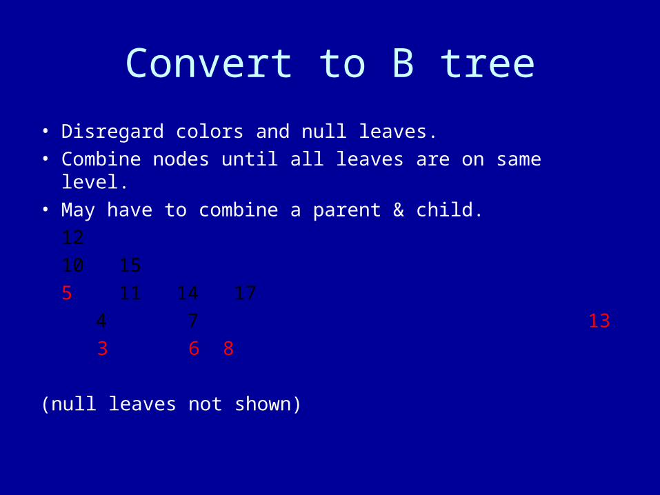
Convert to B tree

• Disregard colors and null leaves.• Combine nodes until all leaves are on same level.• May have to combine a parent & child.

12

10 15

5 11 14 17

4 7 13

3 6 8

(null leaves not shown)

Height of tree

• Is the height = O(log n) where n is the number of nodes? Yes.

• Adding null leaves adds just 1 to the height. Doesn’t really matter if you count them or not. But for “worst case” analysis we should.

• We already know the height of a B tree is O(log n).• Converting (2, 4) B tree to red-black tree could at worst

double the height.• 2 O(log n) + 1 is still O(log n).

Insertion

insert(x):• Replace appropriate null leaf with new “internal” node x.• If x is the root (first insertion), make it black. Otherwise x is red.

– Children of x are black.• The only problem might be if x’s parent is also red. This is called a

“double red”. If no double red, we’re done.• To fix the double red:

Let y = x’s parent, z = x’s grandparent, u = x’s uncle.

2 cases to consider:– Black uncle, or– Red uncle

Look at uncle

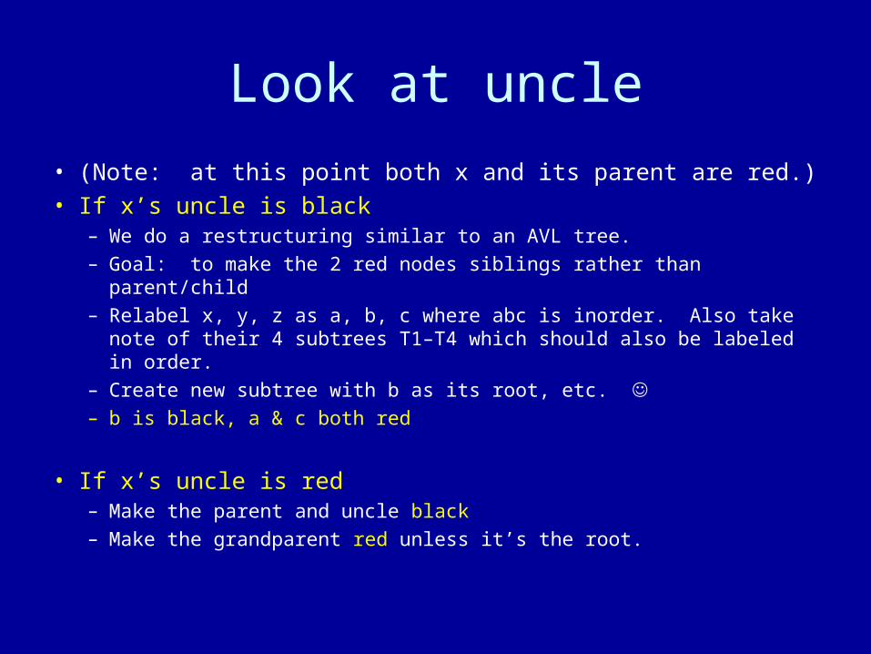
• (Note: at this point both x and its parent are red.)• If x’s uncle is black

– We do a restructuring similar to an AVL tree.– Goal: to make the 2 red nodes siblings rather than parent/child– Relabel x, y, z as a, b, c where abc is inorder. Also take note of

their 4 subtrees T1–T4 which should also be labeled in order.– Create new subtree with b as its root, etc. – b is black, a & c both red

• If x’s uncle is red– Make the parent and uncle black– Make the grandparent red unless it’s the root.

Red-black trees (2)

•Review insertion•Deletion

Example

• Let’s insert these values into an initially empty red-black tree.

4, 7, 12, 15, 3, 5, 14, 18, 16, 17

bu ru bu ru bu ru/bu

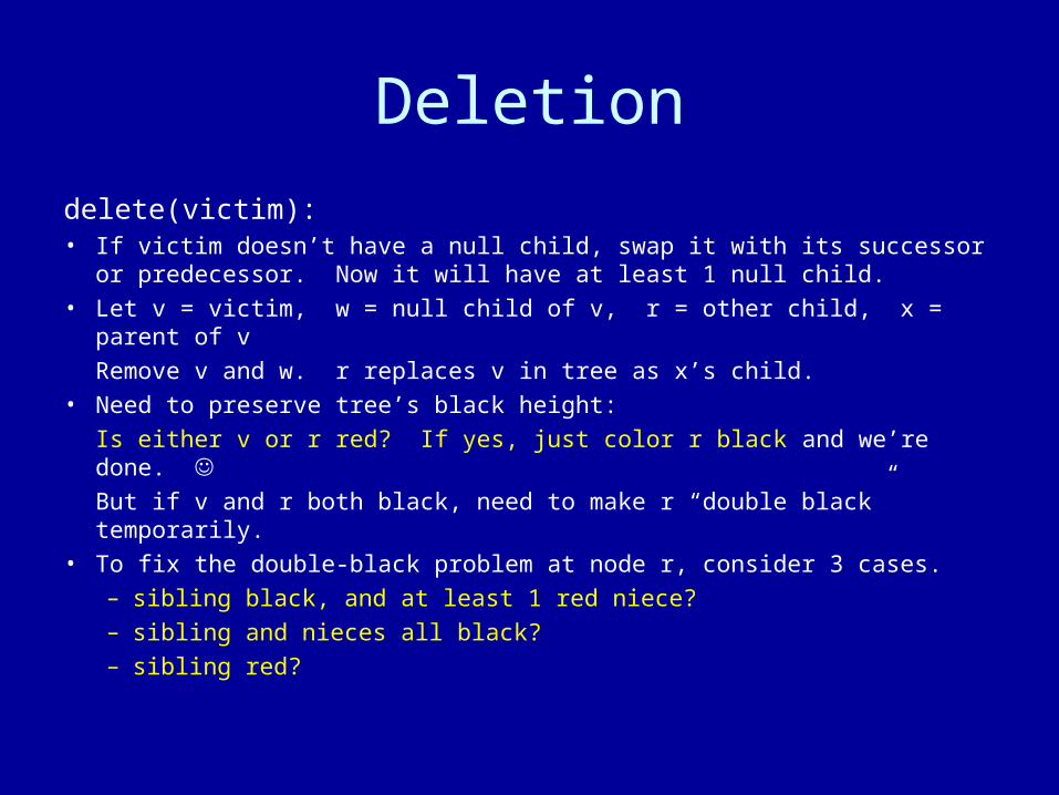
Deletion

delete(victim):• If victim doesn’t have a null child, swap it with its successor or

predecessor. Now it will have at least 1 null child.• Let v = victim, w = null child of v, r = other child, x = parent of v

Remove v and w. r replaces v in tree as x’s child.• Need to preserve tree’s black height:

Is either v or r red? If yes, just color r black and we’re done. But if v and r both black, need to make r “double black” temporarily.

• To fix the double-black problem at node r, consider 3 cases.– sibling black, and at least 1 red niece?– sibling and nieces all black?– sibling red?

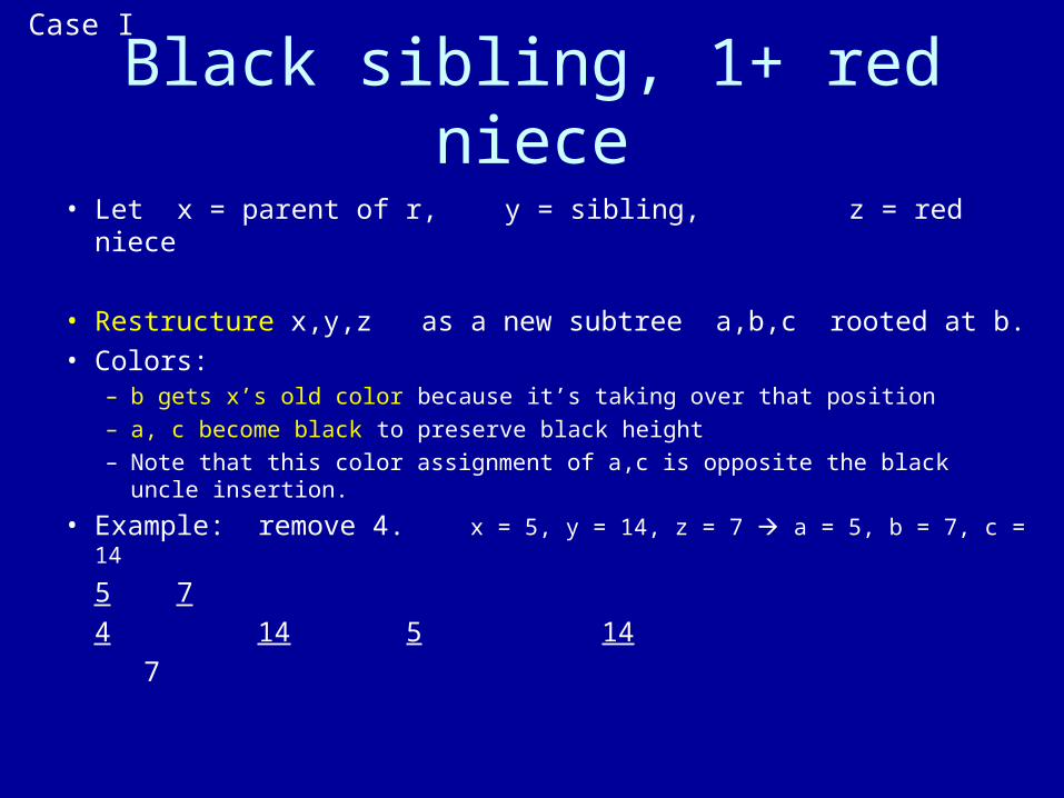
Black sibling, 1+ red niece

• Let x = parent of r, y = sibling, z = red niece

• Restructure x,y,z as a new subtree a,b,c rooted at b.• Colors:

– b gets x’s old color because it’s taking over that position– a, c become black to preserve black height– Note that this color assignment of a,c is opposite the black uncle

insertion.

• Example: remove 4. x = 5, y = 14, z = 7 a = 5, b = 7, c = 14

5 7

4 14 5 14

7

Case I

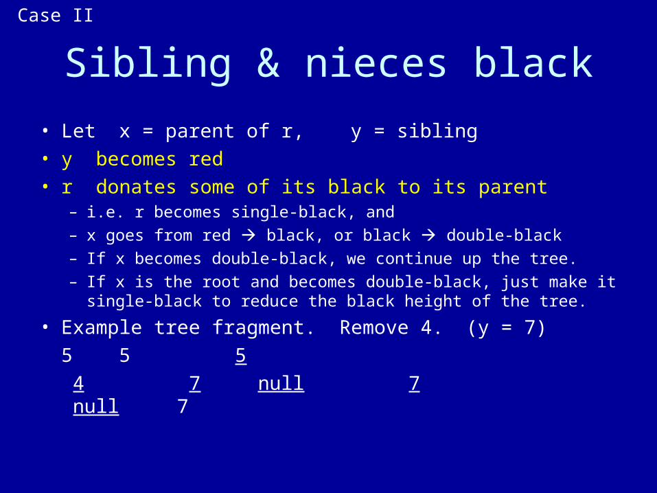
Sibling & nieces black

• Let x = parent of r, y = sibling• y becomes red• r donates some of its black to its parent

– i.e. r becomes single-black, and – x goes from red black, or black double-black– If x becomes double-black, we continue up the tree.– If x is the root and becomes double-black, just make it single-

black to reduce the black height of the tree.

• Example tree fragment. Remove 4. (y = 7)

5 5 5

4 7 null 7 null 7

Case II

Sibling red

• Let x = parent, y = sibling, z = niece on same side as y

• Restructure x,y,z as a,b,c rooted at b.

• Set colors: x = red. This forces new y to be black.

• This does not eliminate the double-black condition. But since y is now black, we have case I or II.

• Example. Remove 4. (x = 5, y = 14, z = 16)

5 14

4 14 5 16 Case II

7 16 null 7

Case III

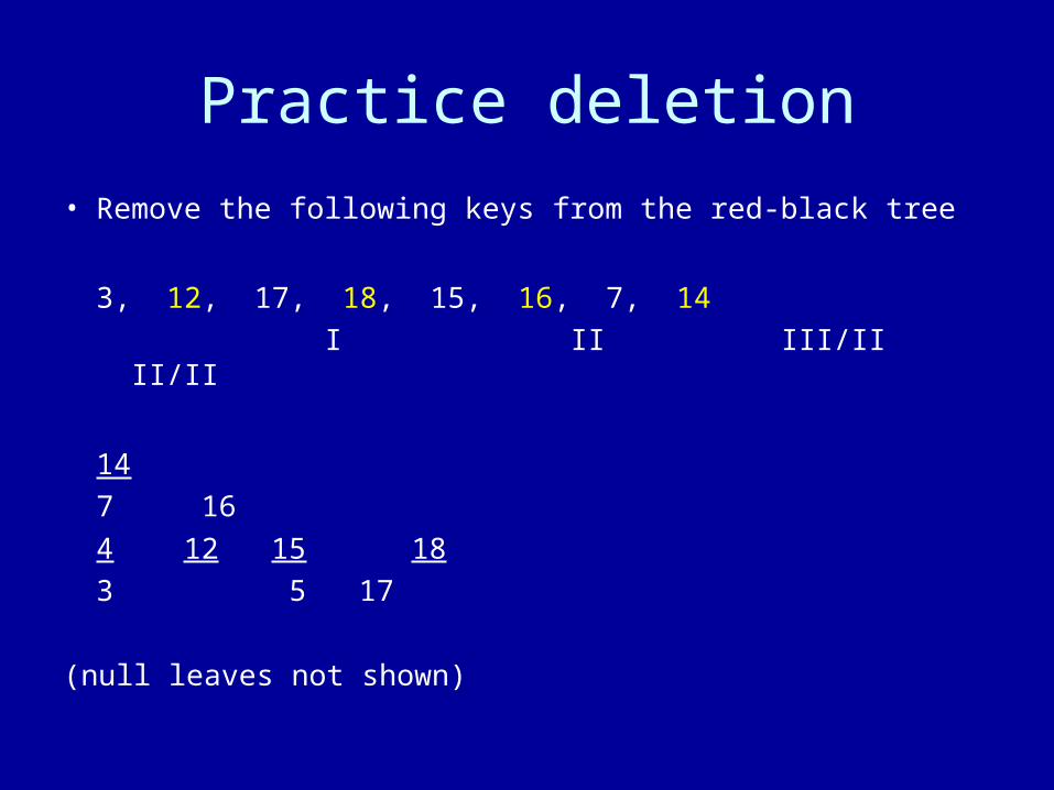
Practice deletion

• Remove the following keys from the red-black tree

3, 12, 17, 18, 15, 16, 7, 14

I II III/II II/II

14

7 16

4 12 15 18

3 5 17

(null leaves not shown)

Splay Trees

• Splay tree is 3rd improvement to BST– Just a BST that we rebalance after each operation– Rationale: we may revisit that node again soon.

– Average case insertion & deletion are O(log n)– Worst case is O(n), because there is no height property

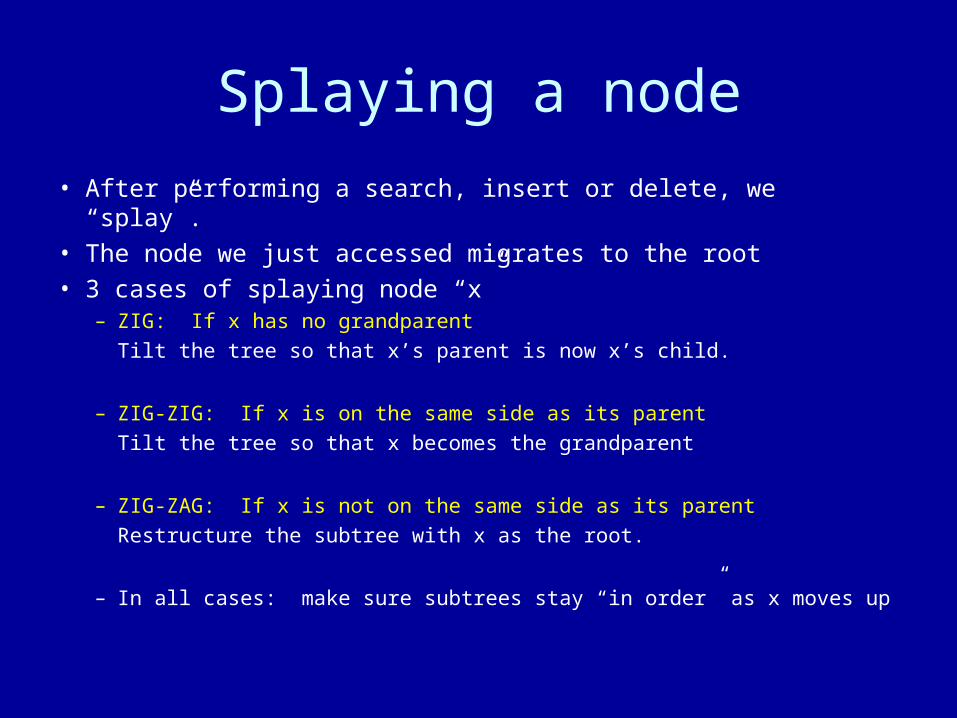
Splaying a node

• After performing a search, insert or delete, we “splay”.

• The node we just accessed migrates to the root

• 3 cases of splaying node “x”– ZIG: If x has no grandparent

Tilt the tree so that x’s parent is now x’s child.

– ZIG-ZIG: If x is on the same side as its parent

Tilt the tree so that x becomes the grandparent

– ZIG-ZAG: If x is not on the same side as its parent

Restructure the subtree with x as the root.

– In all cases: make sure subtrees stay “in order” as x moves up

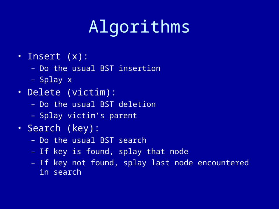
Algorithms

• Insert (x):– Do the usual BST insertion– Splay x

• Delete (victim):– Do the usual BST deletion– Splay victim’s parent

• Search (key):– Do the usual BST search– If key is found, splay that node– If key not found, splay last node encountered in search

Practice

• Start with empty splay tree.

• Insert in succession: 3, 1, 4, 5, 2, 9, 6, 8

• Search for 5

• Remove 1

Skip List

• Skip list is a non-tree alternative to BST– Looks like a 2-d linked list– Randomness is built into the structure

– Definition & example– Operations

Definition

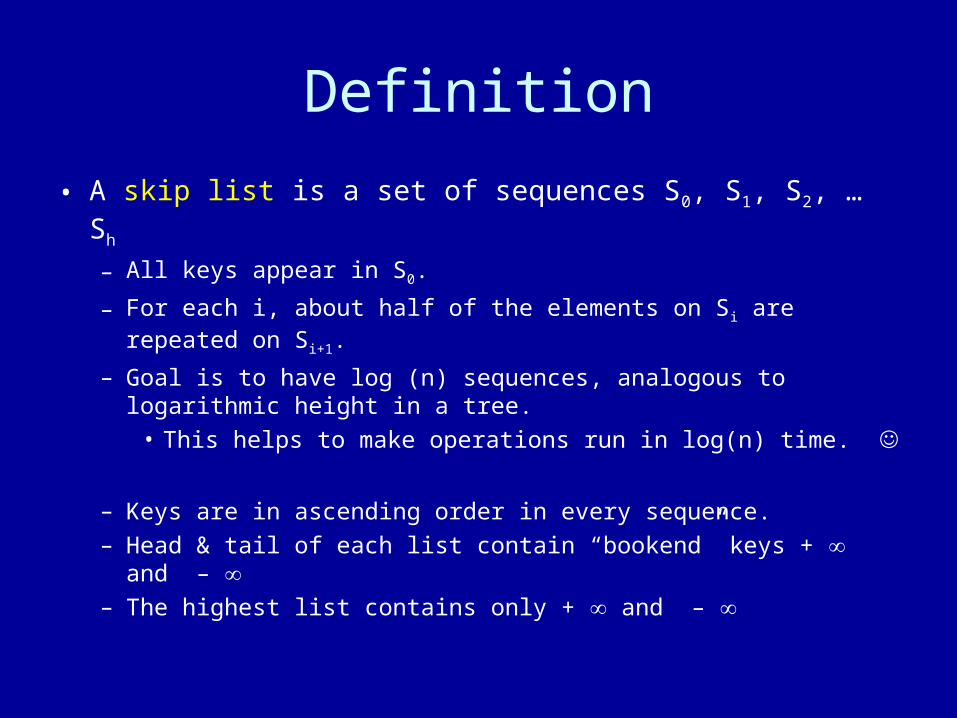
• A skip list is a set of sequences S0, S1, S2, … Sh

– All keys appear in S0.

– For each i, about half of the elements on Si are repeated on Si+1.

– Goal is to have log (n) sequences, analogous to logarithmic height in a tree.

• This helps to make operations run in log(n) time.

– Keys are in ascending order in every sequence.– Head & tail of each list contain “bookend” keys + and – – The highest list contains only + and –

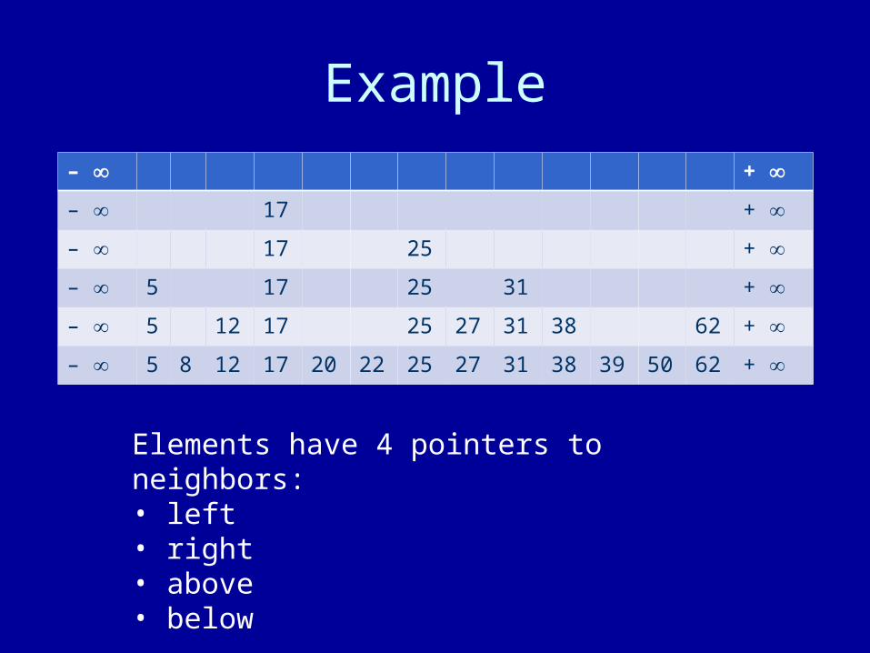
Example

– +

– 17 +

– 17 25 +

– 5 17 25 31 +

– 5 12 17 25 27 31 38 62 +

– 5 8 12 17 20 22 25 27 31 38 39 50 62 +

Elements have 4 pointers to neighbors:• left• right• above• below

Observations

• Skip list does resemble a tree in some respects:– There is a value “on top” that we first encounter, but there could be

more than one.– 2-d pointers are like parent, child, siblings

• To get logarithmic height: we assign a probability of ½ that a value will be repeated on the list above.– Choosing random # saves us the trouble of trying to get the size of

the higher list exactly ½.– Can choose 1 random number at beginning of program, and then

cycle thru its bits.

• There is some waste in duplicating keys, but the items can be stored in the lowest list only. Easy to reach.

Search

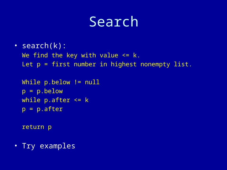
• search(k):We find the key with value <= k.

Let p = first number in highest nonempty list.

While p.below != null

p = p.below

while p.after <= k

p = p.after

return p

• Try examples

Insert & delete

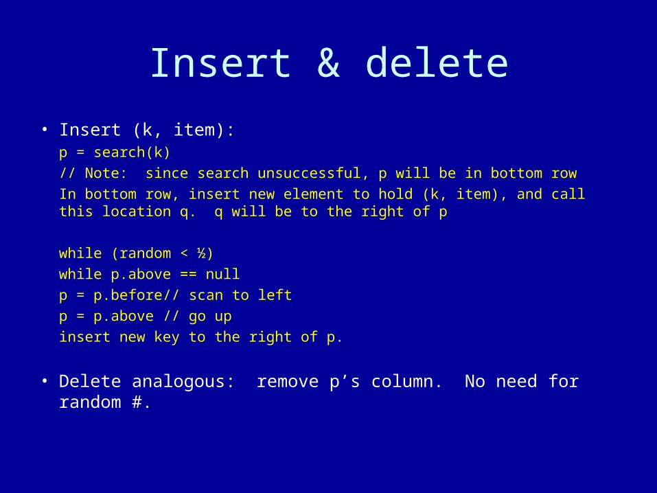
• Insert (k, item):p = search(k)

// Note: since search unsuccessful, p will be in bottom row

In bottom row, insert new element to hold (k, item), and call this location q. q will be to the right of p

while (random < ½)

while p.above == null

p = p.before // scan to left

p = p.above // go up

insert new key to the right of p.

• Delete analogous: remove p’s column. No need for random #.

How good are they?

• Splay tree analysis– Long-term amortized approach, rather than cost of a single

isolated operation

• Skip list analysis– Probabilistic, since the list is built randomly

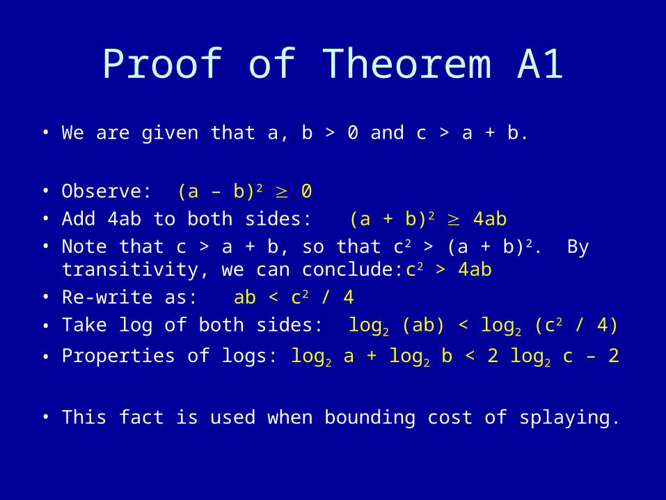
Proof of Theorem A1

• We are given that a, b > 0 and c > a + b.

• Observe: (a – b)2 0• Add 4ab to both sides: (a + b)2 4ab• Note that c > a + b, so that c2 > (a + b)2. By transitivity, we

can conclude: c2 > 4ab• Re-write as: ab < c2 / 4

• Take log of both sides: log2 (ab) < log2 (c2 / 4)

• Properties of logs: log2 a + log2 b < 2 log2 c – 2

• This fact is used when bounding cost of splaying.

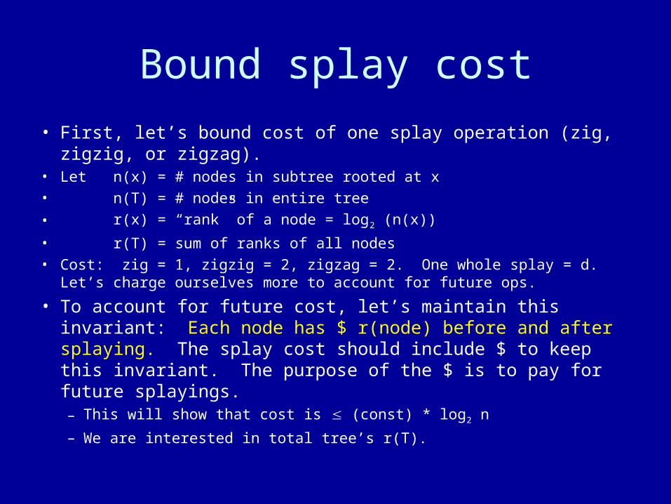
Bound splay cost

• First, let’s bound cost of one splay operation (zig, zigzig, or zigzag).

• Let n(x) = # nodes in subtree rooted at x• n(T) = # nodes in entire tree

• r(x) = “rank” of a node = log2 (n(x))

• r(T) = sum of ranks of all nodes• Cost: zig = 1, zigzig = 2, zigzag = 2. One whole splay = d. Let’s charge

ourselves more to account for future ops.

• To account for future cost, let’s maintain this invariant: Each node has $ r(node) before and after splaying. The splay cost should include $ to keep this invariant. The purpose of the $ is to pay for future splayings.– This will show that cost is (const) * log2 n

– We are interested in total tree’s r(T).

Bound splay cost (2)

• Need to bound the total change in r(T) needed for future splaying.

• What is upper bound for a single splay step (e.g. 1 zig)?• Lemma 3.8: we’ll call this .

• Let r1(x) = old rank of a node x, r2(x) = new rank of x.

• Consider zigzig case. (zigzag is analogous)– 4 subtrees move around, but no net change in rank.– Only x, y, z change rank. Formerly, z was root of subtree, and now

it’s x. x is where z used to be. Thus, r2(x) = r1(z).

– Compute = r2 – r1 of all nodes

– = r2(x) + r2(y) + r2(z) – r1(x) – r1(y) – r1(z)

– = r2(y) + r2(z) – r1(x) – r1(y)

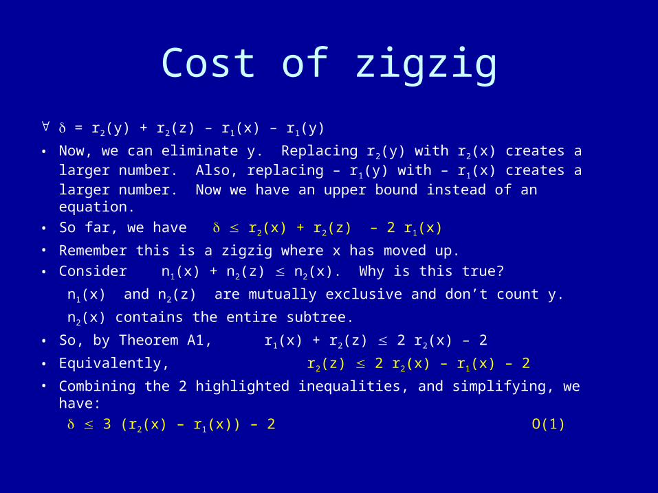
Cost of zigzig

= r2(y) + r2(z) – r1(x) – r1(y)

• Now, we can eliminate y. Replacing r2(y) with r2(x) creates a larger number. Also, replacing – r1(y) with – r1(x) creates a larger number. Now we have an upper bound instead of an equation.

• So far, we have r2(x) + r2(z) – 2 r1(x)

• Remember this is a zigzig where x has moved up.

• Consider n1(x) + n2(z) n2(x). Why is this true?

n1(x) and n2(z) are mutually exclusive and don’t count y.

n2(x) contains the entire subtree.

• So, by Theorem A1, r1(x) + r2(z) 2 r2(x) – 2

• Equivalently, r2(z) 2 r2(x) – r1(x) – 2

• Combining the 2 highlighted inequalities, and simplifying, we have:

3 (r2(x) – r1(x)) – 2 O(1)

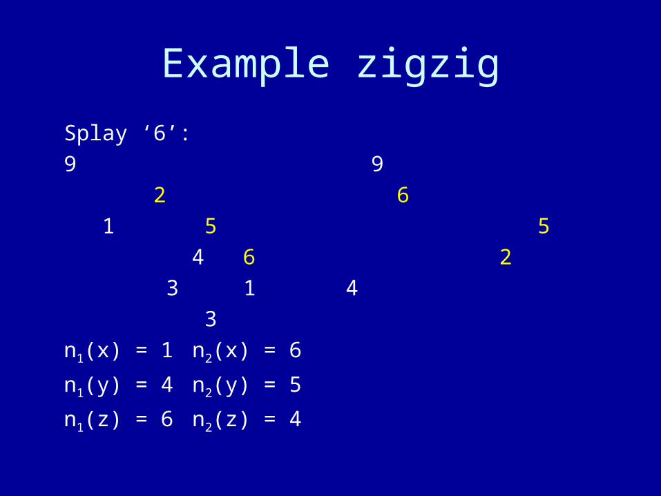
Example zigzig

Splay ‘6’:

9 9

2 6

1 5 5

4 6 2

3 1 4

3

n1(x) = 1 n2(x) = 6

n1(y) = 4 n2(y) = 5

n1(z) = 6 n2(z) = 4

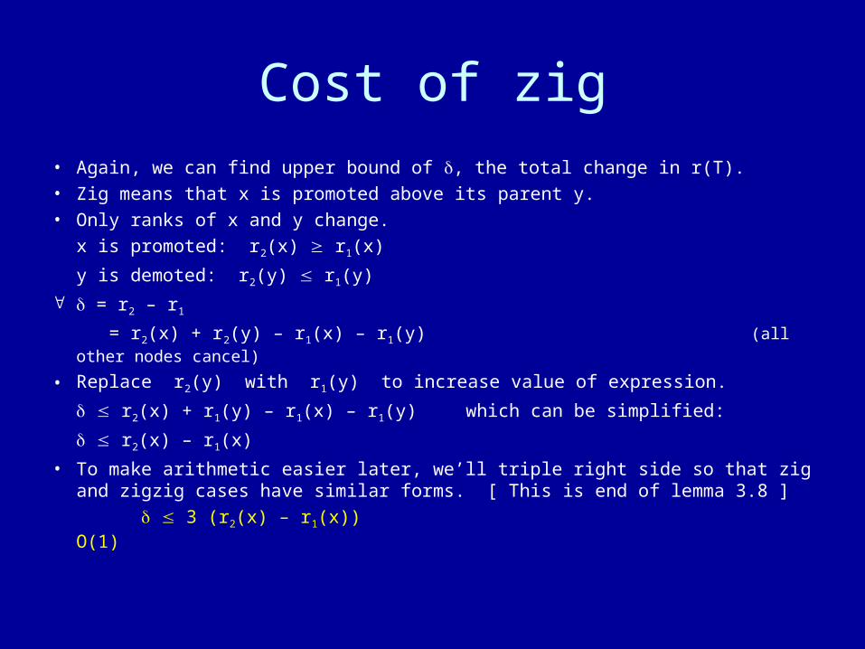
Cost of zig

• Again, we can find upper bound of , the total change in r(T).• Zig means that x is promoted above its parent y.• Only ranks of x and y change.

x is promoted: r2(x) r1(x)

y is demoted: r2(y) r1(y)

= r2 – r1

= r2(x) + r2(y) – r1(x) – r1(y) (all other nodes cancel)

• Replace r2(y) with r1(y) to increase value of expression.

r2(x) + r1(y) – r1(x) – r1(y) which can be simplified:

r2(x) – r1(x)

• To make arithmetic easier later, we’ll triple right side so that zig and zigzig cases have similar forms. [ This is end of lemma 3.8 ]

3 (r2(x) – r1(x)) O(1)

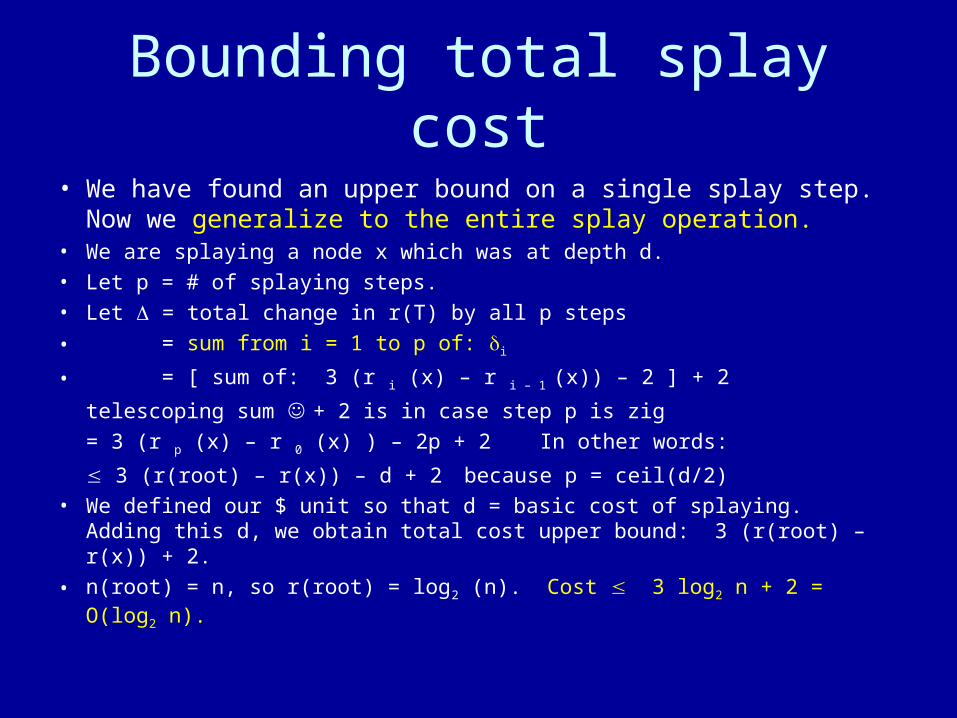
Bounding total splay cost

• We have found an upper bound on a single splay step. Now we generalize to the entire splay operation.

• We are splaying a node x which was at depth d.• Let p = # of splaying steps.• Let = total change in r(T) by all p steps

• = sum from i = 1 to p of: i

• = [ sum of: 3 (r i (x) – r i – 1 (x)) – 2 ] + 2

telescoping sum + 2 is in case step p is zig

= 3 (r p (x) – r 0 (x) ) – 2p + 2 In other words:

3 (r(root) – r(x)) – d + 2 because p = ceil(d/2)• We defined our $ unit so that d = basic cost of splaying. Adding this d, we

obtain total cost upper bound: 3 (r(root) – r(x)) + 2.

• n(root) = n, so r(root) = log2 (n). Cost 3 log2 n + 2 = O(log2 n).

Insertion

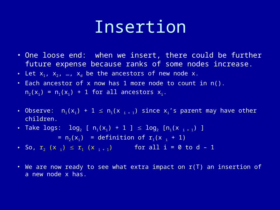
• One loose end: when we insert, there could be further future expense because ranks of some nodes increase.

• Let x1, x2, …, xd be the ancestors of new node x.

• Each ancestor of x now has 1 more node to count in n().

n2(xi) = n1(xi) + 1 for all ancestors xi.

• Observe: n1(xi) + 1 n1(x i + 1) since xi’s parent may have other children.

• Take logs: log2 [ n1(xi) + 1 ] log2 [n1(x i + 1) ]

= n2(xi) = definition of r1(x i + 1)

• So, r2 (x i) r1 (x i + 1) for all i = 0 to d – 1

• We are now ready to see what extra impact on r(T) an insertion of a new node x has.

Bound additional cost

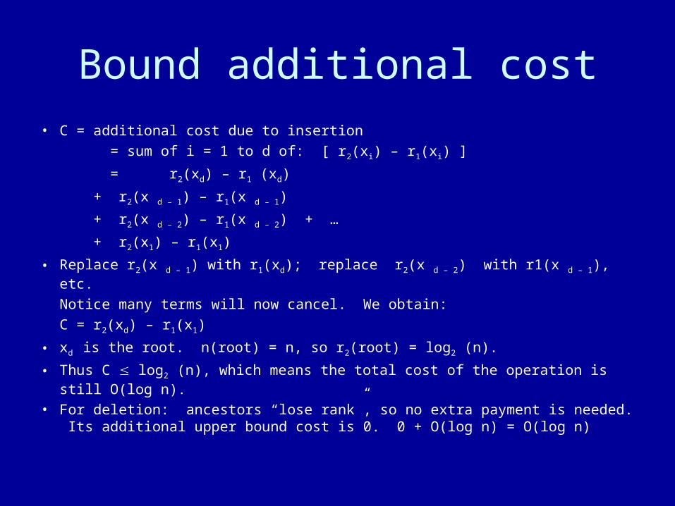
• C = additional cost due to insertion

= sum of i = 1 to d of: [ r2(xi) – r1(xi) ]

= r2(xd) – r1 (xd)

+ r2(x d – 1) – r1(x d – 1)

+ r2(x d – 2) – r1(x d – 2) + …

+ r2(x1) – r1(x1)

• Replace r2(x d – 1) with r1(xd); replace r2(x d – 2) with r1(x d – 1), etc.

Notice many terms will now cancel. We obtain:

C = r2(xd) – r1(x1)

• xd is the root. n(root) = n, so r2(root) = log2 (n).

• Thus C log2 (n), which means the total cost of the operation is still O(log n).

• For deletion: ancestors “lose rank”, so no extra payment is needed. Its additional upper bound cost is 0. 0 + O(log n) = O(log n)

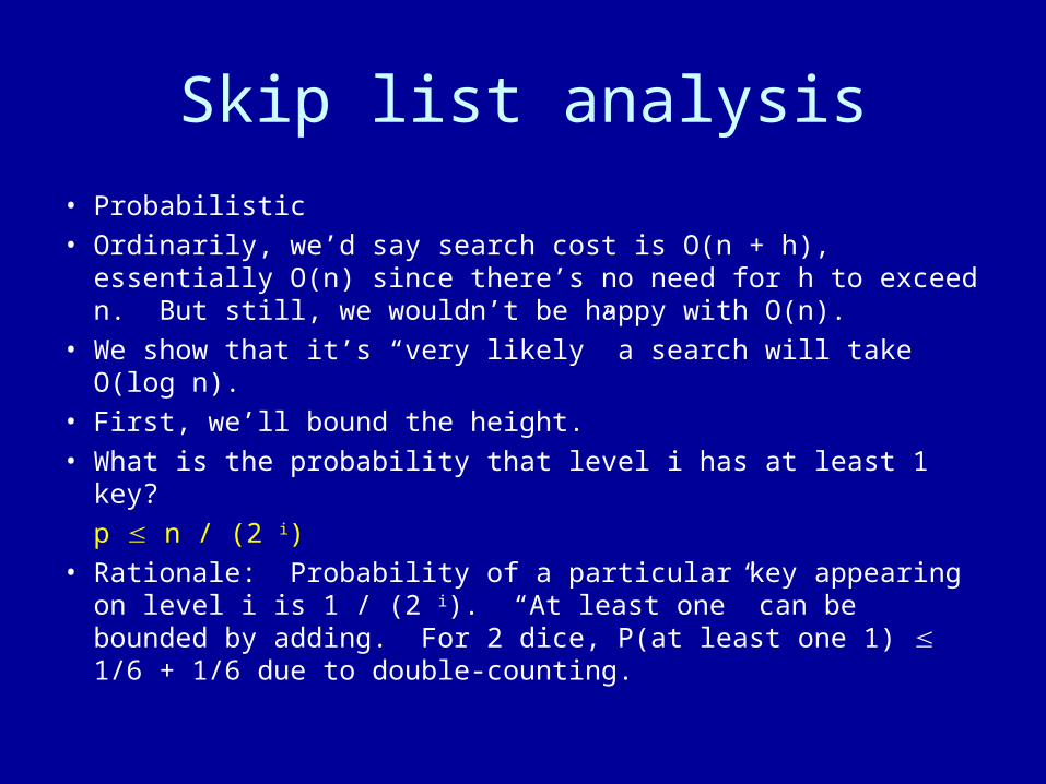
Skip list analysis

• Probabilistic• Ordinarily, we’d say search cost is O(n + h), essentially

O(n) since there’s no need for h to exceed n. But still, we wouldn’t be happy with O(n).

• We show that it’s “very likely” a search will take O(log n).• First, we’ll bound the height.• What is the probability that level i has at least 1 key?

p n / (2 i)• Rationale: Probability of a particular key appearing on level

i is 1 / (2 i). “At least one” can be bounded by adding. For 2 dice, P(at least one 1) 1/6 + 1/6 due to double-counting.

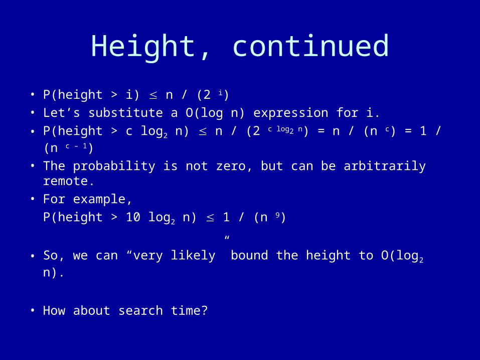
Height, continued

• P(height > i) n / (2 i)• Let’s substitute a O(log n) expression for i.

• P(height > c log2 n) n / (2 c log2 n) = n / (n c) = 1 / (n c – 1)

• The probability is not zero, but can be arbitrarily remote.• For example,

P(height > 10 log2 n) 1 / (n 9)

• So, we can “very likely” bound the height to O(log2 n).

• How about search time?

Skip search

• Outer loop goes “down” a level, so its # iters = O(log2 n)

• Inner loop walks to right.– How many keys do we encounter on level i ?– These are keys that failed to be replicated on row above.– The probability that a key is encountered in this row (instead of a

higher one) is ½.

– How many times do we flip coin until it’s heads?

Draw tree of possibilities…. P(1) = ½, P(2) = ¼, P(3) = 1/8, …

Expected value = familiar sum = 2– So, the number of iterations is O(1).

• Total complexity is O(log2 n) * O(1) = O(log2 n)