Embed Size (px)
Citation preview

CS 372: Computational GeometryLecture 8
Introduction to Randomized Incremental Algorithms
Antoine Vigneron
King Abdullah University of Science and Technology
October 17, 2012
Antoine Vigneron (KAUST) CS 372 Lecture 8 October 17, 2012 1 / 33

1 Introduction
2 Randomized Incremental Quicksort
3 Random Binary Search Trees and History Graphs
Antoine Vigneron (KAUST) CS 372 Lecture 8 October 17, 2012 2 / 33

Course Information
In blackboard:I You have a partial class participation grade (CP1), which will count for
half of the final class participation grade.I There is an average for your grades so far, using 50% for the midterm,
20% for each homework and 10% for CP1.
Final grade:
A A- B+ B B- C+ C C-
85–100 70–85 60–70 50–60 40–50 30–40 25–30 20–25
Antoine Vigneron (KAUST) CS 372 Lecture 8 October 17, 2012 3 / 33

Outline
Randomized incremental constructions are introduced.
Simple example: a modified quicksort.
New techniques:I Random permutation.I Backwards analysis.
Data structures:I Conflict list, history graph.I Random binary search trees.
Reference (this lecture differs substantially) :
Textbook Chapter 6.
Dave Mount’s lecture notes, lectures 14, 15 and 18.
Closer reference: Mulmuley’s textbook Chapter 1.
Antoine Vigneron (KAUST) CS 372 Lecture 8 October 17, 2012 4 / 33
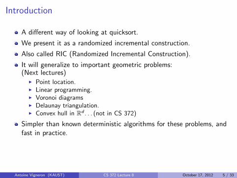
Introduction
A different way of looking at quicksort.
We present it as a randomized incremental construction.
Also called RIC (Randomized Incremental Construction).
It will generalize to important geometric problems:(Next lectures)
I Point location.I Linear programming.I Voronoi diagramsI Delaunay triangulation.I Convex hull in Rd . . . (not in CS 372)
Simpler than known deterministic algorithms for these problems, andfast in practice.
Antoine Vigneron (KAUST) CS 372 Lecture 8 October 17, 2012 5 / 33
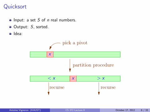
Quicksort
Input: a set S of n real numbers.
Output: S , sorted.
Idea:
x
x< x > x
partition procedure
pick a pivot
recurse recurse
Antoine Vigneron (KAUST) CS 372 Lecture 8 October 17, 2012 6 / 33

Randomization
Usual Quicksort: Pick a pivot at random at each step.
Here: First compute a random permutation of S .I Input: A set S of n real numbers.I Output: A permutation (x1, x2 . . . xn) of S , chosen uniformly at
random.
Random permutation:
First step of the RIC.
This is the only random aspect of the RIC.
Expected running time: The expectation is the average over the n!possible permutations.
I It does not depend on the input.
Antoine Vigneron (KAUST) CS 372 Lecture 8 October 17, 2012 7 / 33

Computing a Random Permutation
Random permutation
Algorithm Permute(A)Input: An array A[1 . . . n] of numbers.Output: A[1 . . . n], randomly permuted.1. for i = n downto 22. do j ← random integer in 1, . . . , i3. Swap(A[i],A[j])
Runs in Θ(n) time.
Generates each permutation with probability 1/n!.
After computing Permute(S):I ∀x ∈ S , ∀i , we have Pr(x = xi ) = 1/n.I We denote Si = x1, x2 . . . xi.
Antoine Vigneron (KAUST) CS 372 Lecture 8 October 17, 2012 8 / 33
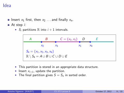
Idea
Insert x1 first, then x2 . . . and finally xn.
At step i :I Si partitions R into i + 1 intervals.
A B C = (x3, x1) D E
S4 = x1, x2, x3, x4R \ S4 = A ∪ B ∪ C ∪ D ∪ E
x2 x3 x1 x4
I This partition is stored in an appropriate data structure.I Insert xi+1, update the partition.I The final partition gives S = Sn in sorted order.
Antoine Vigneron (KAUST) CS 372 Lecture 8 October 17, 2012 9 / 33

Data Structure: Preliminary
At step i :I Each interval stores pointers to its two endpoints.I For each j 6 i , we store pointers from xj to its two adjacent intervals.
B C
x3
Antoine Vigneron (KAUST) CS 372 Lecture 8 October 17, 2012 10 / 33
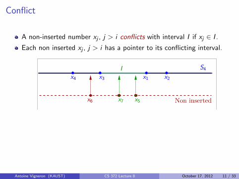
Conflict
A non-inserted number xj , j > i conflicts with interval I if xj ∈ I .
Each non inserted xj , j > i has a pointer to its conflicting interval.
I
x6
S4
x7 x5 Non inserted
x4 x3 x1 x2
Antoine Vigneron (KAUST) CS 372 Lecture 8 October 17, 2012 11 / 33
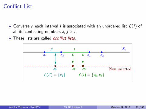
Conflict List
Conversely, each interval I is associated with an unordered list L(I ) ofall its conflicting numbers xj ,j > i .
These lists are called conflict lists.
I
x6
S4
x7 x5
I ′
L(I ′) = x6 L(I ) = x5, x7Non inserted
x4 x3 x1 x2
Antoine Vigneron (KAUST) CS 372 Lecture 8 October 17, 2012 12 / 33
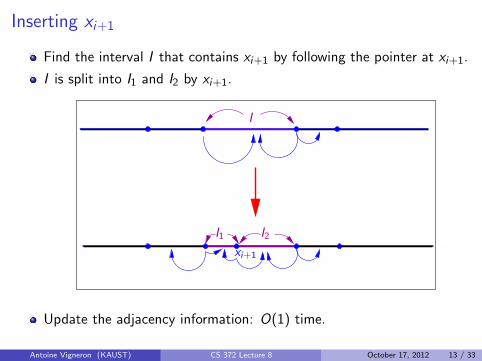
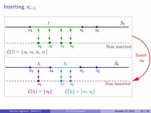
Inserting xi+1
Find the interval I that contains xi+1 by following the pointer at xi+1.
I is split into I1 and I2 by xi+1.
I
I2I1
xi+1
Update the adjacency information: O(1) time.
Antoine Vigneron (KAUST) CS 372 Lecture 8 October 17, 2012 13 / 33

Inserting xi+1
Build L(I1) and L(I2):
Traverse L(I ), for each element check if it lies in I1 or I2, and insert itin the appropriate conflict list.
It takes O(|L(I )|) time.
At the same time, we update the pointer between each xj in L(I ) tothe new conflicting interval I1 or I2.
Antoine Vigneron (KAUST) CS 372 Lecture 8 October 17, 2012 14 / 33
Inserting xi+1
S3
x6 x7 x5
I
L(I ) = x6, x4, x5, x7
I2
x7 x5x6
I1
Non inserted
S4x4
L(I1) = x6 L(I2) = x7, x5
Non inserted
Insert
x3 x1 x2
x4
x3 x4 x1 x2
Antoine Vigneron (KAUST) CS 372 Lecture 8 October 17, 2012 15 / 33
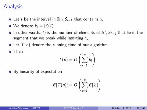
Analysis
Let I be the interval in R \ Si−1 that contains xi .
We denote ki = |L(I )|.In other words, ki is the number of elements of S \ Si−1 that lie in thesegment that we break while inserting xi .
Let T (n) denote the running time of our algorithm.
Then
T (n) = O
(n∑
i=1
ki
).
By linearity of expectation
E [T (n)] = O
(n∑
i=1
E [ki ]
).
Antoine Vigneron (KAUST) CS 372 Lecture 8 October 17, 2012 16 / 33
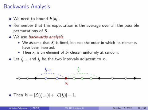
Backwards Analysis
We need to bound E [ki ].
Remember that this expectation is the average over all the possiblepermutations of S .
We use backwards analysis.I We assume that Si is fixed, but not the order in which its elements
have been inserted.I Then xi is an element of Si chosen uniformly at random.
Let Ij−1 and Ij be the two intervals adjacent to xi .
xi
Ij−1 Ij
Then ki = |L(Ij−1)|+ |L(Ij)|+ 1.
Antoine Vigneron (KAUST) CS 372 Lecture 8 October 17, 2012 17 / 33
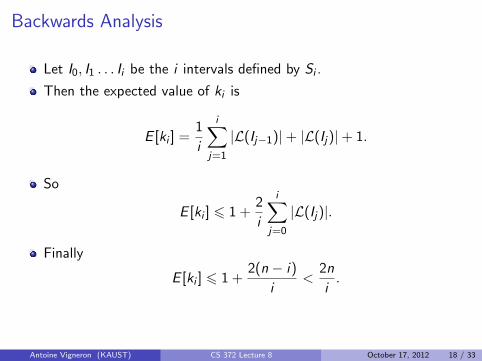
Backwards Analysis
Let I0, I1 . . . Ii be the i intervals defined by Si .
Then the expected value of ki is
E [ki ] =1
i
i∑j=1
|L(Ij−1)|+ |L(Ij)|+ 1.
So
E [ki ] 6 1 +2
i
i∑j=0
|L(Ij)|.
Finally
E [ki ] 6 1 +2(n − i)
i<
2n
i.
Antoine Vigneron (KAUST) CS 372 Lecture 8 October 17, 2012 18 / 33
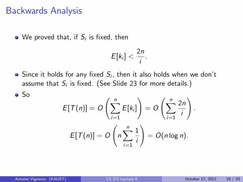
Backwards Analysis
We proved that, if Si is fixed, then
E [ki ] <2n
i.
Since it holds for any fixed Si , then it also holds when we don’tassume that Si is fixed. (See Slide 23 for more details.)
So
E [T (n)] = O
(n∑
i=1
E [ki ]
)= O
(n∑
i=1
2n
i
).
E [T (n)] = O
(n
n∑i=1
1
i
)= O(n log n).
Antoine Vigneron (KAUST) CS 372 Lecture 8 October 17, 2012 19 / 33

Backwards Analysis: Example
Let S = 1, 2, 3, 4, 5, 6, 7.First case: assume S3 = 2, 4, 7.
I So (x1, x2, x3) is a random permutation of 2, 4, 7,and (x4 . . . x7) is a random permutation of 1, 3, 5, 6.
I What is E [k3] under this assumption?I Three possibilities are equally likely: x3 = 2, or x3 = 4 or x3 = 7.
F If x3 = 2, then k3 = 3.F If x3 = 4, then k3 = 4.F If x3 = 7, then k3 = 3
I So
E [k3] =10
3
6 1 +2(n − i)
i
=11
3.
Antoine Vigneron (KAUST) CS 372 Lecture 8 October 17, 2012 20 / 33
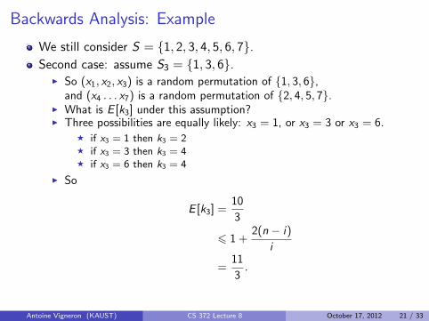
Backwards Analysis: Example
We still consider S = 1, 2, 3, 4, 5, 6, 7.Second case: assume S3 = 1, 3, 6.
I So (x1, x2, x3) is a random permutation of 1, 3, 6,and (x4 . . . x7) is a random permutation of 2, 4, 5, 7.
I What is E [k3] under this assumption?I Three possibilities are equally likely: x3 = 1, or x3 = 3 or x3 = 6.
F if x3 = 1 then k3 = 2F if x3 = 3 then k3 = 4F if x3 = 6 then k3 = 4
I So
E [k3] =10
3
6 1 +2(n − i)
i
=11
3.
Antoine Vigneron (KAUST) CS 372 Lecture 8 October 17, 2012 21 / 33
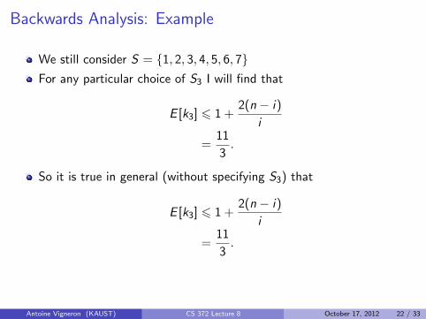
Backwards Analysis: Example
We still consider S = 1, 2, 3, 4, 5, 6, 7For any particular choice of S3 I will find that
E [k3] 6 1 +2(n − i)
i
=11
3.
So it is true in general (without specifying S3) that
E [k3] 6 1 +2(n − i)
i
=11
3.
Antoine Vigneron (KAUST) CS 372 Lecture 8 October 17, 2012 22 / 33

Backwards Analysis: More Detailed Proof
In Slide 19, we showed that for any F ⊂ S such that |F | = i , we have
E [ki | Si = F ] <2n
i.
We can rewrite it ∑k
k .P[ki = k | Si = F ] <2n
i,
and thus ∑k
kP[ki = k ,Si = F ]
P[Si = F ]<
2n
i.
Antoine Vigneron (KAUST) CS 372 Lecture 8 October 17, 2012 23 / 33
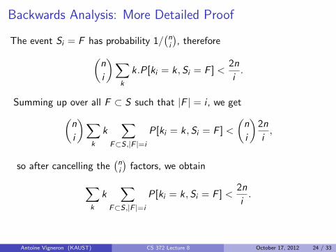
Backwards Analysis: More Detailed Proof
The event Si = F has probability 1/(ni
), therefore(
n
i
)∑k
k .P[ki = k ,Si = F ] <2n
i.
Summing up over all F ⊂ S such that |F | = i , we get(n
i
)∑k
k∑
F⊂S,|F |=i
P[ki = k , Si = F ] <
(n
i
)2n
i,
so after cancelling the(ni
)factors, we obtain∑
k
k∑
F⊂S,|F |=i
P[ki = k , Si = F ] <2n
i.
Antoine Vigneron (KAUST) CS 372 Lecture 8 October 17, 2012 24 / 33

Backwards Analysis: More Detailed Proof
As the events Si = F are mutually exclusive, we can rewrite it∑k
k.P[ki = k] <2n
i,
and thus
E [ki ] <2n
i.
Antoine Vigneron (KAUST) CS 372 Lecture 8 October 17, 2012 25 / 33
Concluding Remarks
The expected running time is O(n log n).
It works on any input.
So this is an expected running time on worst case input.
Expectation is over the random choices of the algorithm.
On the other hand, deterministic quicksort (with fixed pivot):
Sorts random input in expected O(n log n) time.
But is quadratic on worst case input.
Antoine Vigneron (KAUST) CS 372 Lecture 8 October 17, 2012 26 / 33
Motivation
We solved sorting using RIC.
Is there a related query problem?
Yes, searching.
Formulation:I S defines a partition of R into intervals.I Given a query number q, which interval does it belong to?I General position assumption: q /∈ S .
Can be solved simply by binary search.
Here we give a method that can be generalized to solve more difficultproblems. (See next lecture).
Antoine Vigneron (KAUST) CS 372 Lecture 8 October 17, 2012 27 / 33

Idea
During the RIC, after we split an interval, we forget it.
Now we will store the information in a history graph.
(In our case, this graph is a tree.)
Now, if we split I into I` and Ir :I Make two nodes containing I` and Ir respectively.I Draw edges (I , I`) and (I,Ir ).
xi
I`
I
Ir
I
I`Ir
Antoine Vigneron (KAUST) CS 372 Lecture 8 October 17, 2012 28 / 33

Example
History graph
x1x2 x5 x3 x4
x1
x2
x3
x4
x5
(−∞,∞)
(x1,∞)(−∞, x1)
(−∞, x2) (x2, x1) (x1, x3) (x3,∞)
(x3, x4) (x4,∞)(x2, x5) (x5, x1)
Antoine Vigneron (KAUST) CS 372 Lecture 8 October 17, 2012 29 / 33

Answering queries
q denotes the query number.
Start at the root.I If the current node is a leaf, we are done.I Find the child whose interval contains q.I Recurse on this node.
We have just build a randomized binary search tree.
Query time?I Worst case: Ω(n).I Best case: O(1).I Average: O(log n). (See next slides.)
Antoine Vigneron (KAUST) CS 372 Lecture 8 October 17, 2012 30 / 33

Analysis
Expectation will be over the random choice of the permutation of S .
We consider that q is fixed and the data structure is random.
We denote by Ji the interval defined by Si that contains q.
That is, the interval that contains q at the i–th step of the RIC.
The number of different intervals Ji gives the number of nodes in thesearch path, hence the query time.
What is the probability that Ji 6= Ji−1?I It is the probability that Ji−1 is split while inserting xi .
Antoine Vigneron (KAUST) CS 372 Lecture 8 October 17, 2012 31 / 33
Backwards Analysis
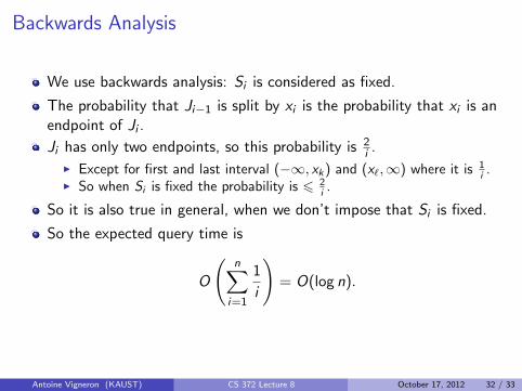
We use backwards analysis: Si is considered as fixed.
The probability that Ji−1 is split by xi is the probability that xi is anendpoint of Ji .
Ji has only two endpoints, so this probability is 2i .
I Except for first and last interval (−∞, xk) and (x`,∞) where it is 1i .
I So when Si is fixed the probability is 6 2i .
So it is also true in general, when we don’t impose that Si is fixed.
So the expected query time is
O
(n∑
i=1
1
i
)= O(log n).
Antoine Vigneron (KAUST) CS 372 Lecture 8 October 17, 2012 32 / 33
Concluding Remarks
We have shown that, for a fixed query point, the search path hasexpected length O(log n).
It is also true that the expected length of the longest search path isO(log n), and that it holds with high probability.
In other words the height of a random BST is O(log n), like abalanced BST.
Problem: we cannot insert or delete in a random BST and keep thisbound. Why?
I In this case, the insertion order is not random.I So insertion can take Ω(n) time and height can be Ω(n) time too.
Antoine Vigneron (KAUST) CS 372 Lecture 8 October 17, 2012 33 / 33