Embed Size (px)
Citation preview

CS 416Artificial Intelligence
Lecture 17Lecture 17
Reasoning over TimeReasoning over Time
Chapter 15Chapter 15
Lecture 17Lecture 17
Reasoning over TimeReasoning over Time
Chapter 15Chapter 15

Sampling your way to a solution
As time proceeds, you collect informationAs time proceeds, you collect information
• XXtt – The variables you cannot observe (at time t) – The variables you cannot observe (at time t)
• EEtt – the variables you can observe (at time t) – the variables you can observe (at time t)
– A particular observation is eA particular observation is ett
• XXa:ba:b – indicates set of variables from X – indicates set of variables from Xaa to X to Xbb

Dealing with time
Consider P ( xConsider P ( xtt | e | e0:t 0:t ))
• To construct Bayes NetworkTo construct Bayes Network
– xxtt depends on e depends on ett
– eett depends on e depends on et-1t-1
– eet-1t-1 depends on e depends on et-2t-2
– … … potentially infinite number of parentspotentially infinite number of parents
• Avoid this by making an assumption!Avoid this by making an assumption!

Markov assumption
The current state depends only on a finite history The current state depends only on a finite history of previous statesof previous states
• First-orderFirst-order Markov processMarkov process: the current state depends only : the current state depends only on the previous stateon the previous state
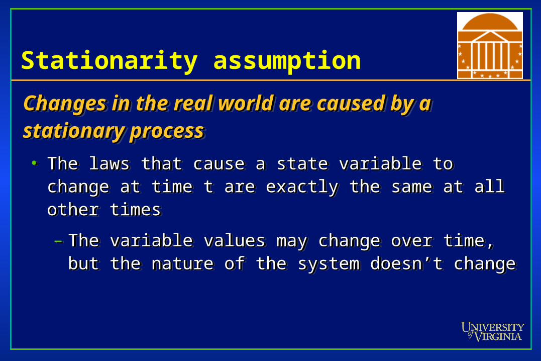
Stationarity assumption
Changes in the real world are caused by a Changes in the real world are caused by a stationary processstationary process
• The laws that cause a state variable to change at time t are The laws that cause a state variable to change at time t are exactly the same at all other timesexactly the same at all other times
– The variable values may change over time, but the nature The variable values may change over time, but the nature of the system doesn’t changeof the system doesn’t change

Models of state transitions
State transition modelState transition model
•
Sensor modelSensor model
•
• Evidence variables depend only on the current stateEvidence variables depend only on the current state
–
• The actual state of the world The actual state of the world causes causes the evidence valuesthe evidence values
State transition modelState transition model
•
Sensor modelSensor model
•
• Evidence variables depend only on the current stateEvidence variables depend only on the current state
–
• The actual state of the world The actual state of the world causes causes the evidence valuesthe evidence values

Initial Conditions
Specify a prior probability over the states at time 0Specify a prior probability over the states at time 0
• P(XP(X00))
Specify a prior probability over the states at time 0Specify a prior probability over the states at time 0
• P(XP(X00))

A complete joint distribution
We knowWe know
• Initial conditions of state variables: P (XInitial conditions of state variables: P (X00))
• Initial observations (evidence variables): Initial observations (evidence variables):
• Transition probabilities:Transition probabilities:
Therefore we have a complete model Therefore we have a complete model

What might we do with our model?FilteringFiltering
• given all evidence to date, compute the belief state of the unobserved variablesgiven all evidence to date, compute the belief state of the unobserved variables: : P(XP(Xtt | e | e1:t1:t))
PredictionPrediction
• Predict the pPredict the posterior distribution of a future state: P(Xosterior distribution of a future state: P(Xt+k t+k | e| e1:t1:t))
SmoothingSmoothing
• Use recent evidence values as hindsight to predict previous values of the Use recent evidence values as hindsight to predict previous values of the unobserved variables: P(Xunobserved variables: P(Xkk | e | e1:t1:t), 0<=k<t), 0<=k<t
Most likely explanationMost likely explanation
• What sequence of states most likely generated the sequence of observations?What sequence of states most likely generated the sequence of observations?argmaxargmaxx1:tx1:t P(x P(x1:t1:t | e | e1:t1:t))
FilteringFiltering
• given all evidence to date, compute the belief state of the unobserved variablesgiven all evidence to date, compute the belief state of the unobserved variables: : P(XP(Xtt | e | e1:t1:t))
PredictionPrediction
• Predict the pPredict the posterior distribution of a future state: P(Xosterior distribution of a future state: P(Xt+k t+k | e| e1:t1:t))
SmoothingSmoothing
• Use recent evidence values as hindsight to predict previous values of the Use recent evidence values as hindsight to predict previous values of the unobserved variables: P(Xunobserved variables: P(Xkk | e | e1:t1:t), 0<=k<t), 0<=k<t
Most likely explanationMost likely explanation
• What sequence of states most likely generated the sequence of observations?What sequence of states most likely generated the sequence of observations?argmaxargmaxx1:tx1:t P(x P(x1:t1:t | e | e1:t1:t))

Filtering / Prediction
Given filtering up to t, can we predict t+1 from new Given filtering up to t, can we predict t+1 from new evidence at t+1?evidence at t+1?
Two steps:Two steps:
• Project state at xProject state at xtt to x to xt+1 t+1 using transition model: P(Xusing transition model: P(X tt | X | Xt-1t-1) )
• Update that projection using eUpdate that projection using e t+1 t+1 and sensor model: P(Eand sensor model: P(Et t | X| Xtt))

Filtering/Projection
• Project state at xProject state at xtt to x to xt+1 t+1 using transition model: P(Xusing transition model: P(X tt | X | Xt-1t-1) )
• Update that projection using eUpdate that projection using e t+1 t+1 and sensor model: P(Eand sensor model: P(Et t | X| Xtt))
• Project state at xProject state at xtt to x to xt+1 t+1 using transition model: P(Xusing transition model: P(X tt | X | Xt-1t-1) )
• Update that projection using eUpdate that projection using e t+1 t+1 and sensor model: P(Eand sensor model: P(Et t | X| Xtt))
sensormodel
transition modelmust solve because wedon’t know Xt
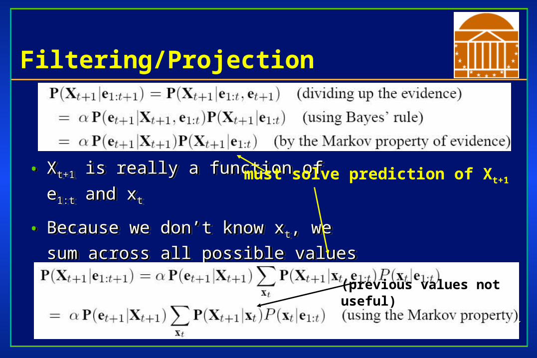
Filtering/Projection
• XXt+1t+1 is really a function of is really a function of
ee1:t1:t and x and xtt
• Because we don’t know xBecause we don’t know x tt, we, we
sum across all possible valuessum across all possible values
• XXt+1t+1 is really a function of is really a function of
ee1:t1:t and x and xtt
• Because we don’t know xBecause we don’t know x tt, we, we
sum across all possible valuessum across all possible values
must solve prediction of Xt+1
(previous values not useful)

Filtering example
Is it rainingIs it rainingtt? Based on observation of umbrella? Based on observation of umbrellatt
• Initial probability, P(RInitial probability, P(R00) = <0.5, 0.5>) = <0.5, 0.5>
• Transition model: Transition model: P (RP (Rt+1t+1 | r | rtt) = <0.7, 0.3>) = <0.7, 0.3>
P (RP (Rt+1t+1 | ~r | ~rtt) = <0.3, 0.7>) = <0.3, 0.7>
• Sensor model: Sensor model: P (RP (Rtt | u | utt) = <0.9, 0.1>) = <0.9, 0.1>
P (RP (Rtt | ~u | ~utt) = <0.2, 0.8>) = <0.2, 0.8>
Given UGiven U11 = TRUE, what is P(R = TRUE, what is P(R11)?)?
• First, predict transition from xFirst, predict transition from x00 to x to x11 and update with evidence and update with evidence

Given U1 = TRUE, what is P(R1)?
Predict transition from xPredict transition from x00 to x to x11
• Because we don’t know xBecause we don’t know x00 we have to consider all cases we have to consider all cases
Predict transition from xPredict transition from x00 to x to x11
• Because we don’t know xBecause we don’t know x00 we have to consider all cases we have to consider all cases
It was rainingIt wasn’t raining

Given U1 = TRUE, what is P(R1)?
Update with evidenceUpdate with evidenceUpdate with evidenceUpdate with evidence
sensormodel
prob. of seeingumbrella givenit was raining
prob. of seeingumbrella givenit wasn’t raining
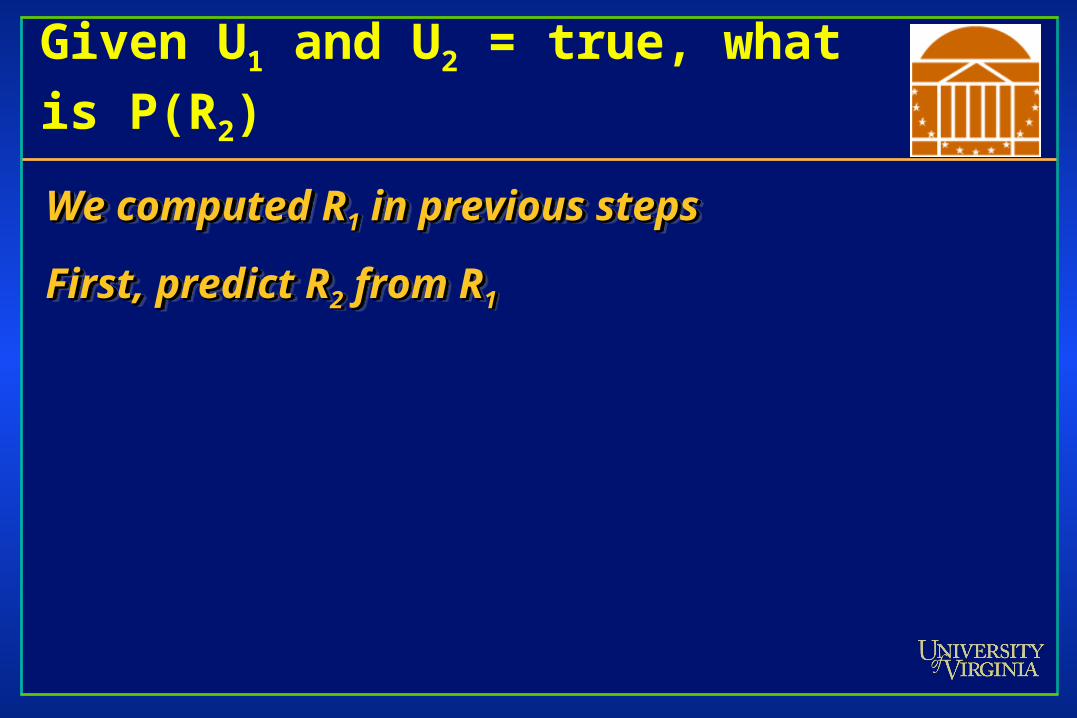
Given U1 and U2 = true, what is P(R2)
We computed RWe computed R11 in previous steps in previous steps
First, predict RFirst, predict R22 from R from R11
We computed RWe computed R11 in previous steps in previous steps
First, predict RFirst, predict R22 from R from R11

Given U1 and U2 = true, what is P(R2)
Second, update RSecond, update R22 with evidence with evidence
When queried to solve for RWhen queried to solve for Rnn
• Use a Use a forwardforward algorithm that recursively solves for R algorithm that recursively solves for R ii for i < n for i < n
Second, update RSecond, update R22 with evidence with evidence
When queried to solve for RWhen queried to solve for Rnn
• Use a Use a forwardforward algorithm that recursively solves for R algorithm that recursively solves for R ii for i < n for i < n
From R1

Prediction
Use evidence 1Use evidence 1t to predict state at t+k+1t to predict state at t+k+1
• For all possible states xFor all possible states xt+k t+k consider the transition model to xconsider the transition model to x t+k+1t+k+1
• For all states xFor all states xt+kt+k consider the likelihood given e consider the likelihood given e1:t1:t

Prediction
Limits of predictionLimits of prediction
• As k increases, a fixed output results – As k increases, a fixed output results – stationary distributionstationary distribution
• The time to reach the stationary distribution – The time to reach the stationary distribution – mixing timemixing time
Limits of predictionLimits of prediction
• As k increases, a fixed output results – As k increases, a fixed output results – stationary distributionstationary distribution
• The time to reach the stationary distribution – The time to reach the stationary distribution – mixing timemixing time

Smoothing
P(XP(Xkk | e | e1:t 1:t ), 0<=k<t), 0<=k<t
• Attack this in two partsAttack this in two parts
– P(XP(Xkk | e | e1:k1:k, e, ek+1:tk+1:t))
P(XP(Xkk | e | e1:t 1:t ), 0<=k<t), 0<=k<t
• Attack this in two partsAttack this in two parts
– P(XP(Xkk | e | e1:k1:k, e, ek+1:tk+1:t))
Bayes
bk+1:t = P(ek+1:t | Xk)
Smoothing
Forward part:Forward part:
• What is probability XWhat is probability Xkk given evidence 1 given evidence 1kk
Backward part:Backward part:
• What is probability of observing evidence k+1What is probability of observing evidence k+1t given Xt given Xkk
How do we compute the backward part?How do we compute the backward part?

Smoothing
Computing the backward partComputing the backward partComputing the backward partComputing the backward part

Whiteboard

Example
Probability rProbability r11 given u given u11 and u and u22Probability rProbability r11 given u given u11 and u and u22
solved for thisin step one of forward soln.

Viterbi
Consider finding the most likely path through a Consider finding the most likely path through a sequence of states given observationssequence of states given observations
Could enumerate all 2Could enumerate all 255 permutations of five-sequence permutations of five-sequence rain/~rain options and evaluate P(xrain/~rain options and evaluate P(x1:51:5 | e | e1:51:5))

Viterbi
Could use Could use smoothingsmoothing to find posterior distribution to find posterior distribution for weather at each time step and create path for weather at each time step and create path through most probable – through most probable – treats each as a single treats each as a single step, not a sequence!step, not a sequence!
Could use Could use smoothingsmoothing to find posterior distribution to find posterior distribution for weather at each time step and create path for weather at each time step and create path through most probable – through most probable – treats each as a single treats each as a single step, not a sequence!step, not a sequence!

Viterbi
Specify a final state and find previous states that form most likely pathSpecify a final state and find previous states that form most likely path
• Let RLet R55 = true = true
• Find RFind R44 such that it is on the optimal path to R such that it is on the optimal path to R55. Consider each value of R. Consider each value of R44
– Evaluate how likely it will lead to REvaluate how likely it will lead to R55=true and how easily it is reached=true and how easily it is reached
Find RFind R33 such that it is on optimal path to R such that it is on optimal path to R44. Consider each value…. Consider each value…

Viterbi – Recursive algorithm

Viterbi - Recursive

Viterbi - Recursive
The Viterbi algorithm is just like the filtering The Viterbi algorithm is just like the filtering algorithm except for two changesalgorithm except for two changes
• Replace fReplace f1:t1:t = P(X = P(Xtt | e | e1:t1:t))
– with:with:
• Summation over xSummation over xtt replaced with max over x replaced with max over xtt

Review
Forward:Forward:
Forward/Backward:Forward/Backward:
Max:Max:
Forward:Forward:
Forward/Backward:Forward/Backward:
Max:Max:

Hidden Markov Models (HMMs)
Represent the state of the world with a single discrete Represent the state of the world with a single discrete variablevariable
• If your state has multiple variables, form one variable whose value takes If your state has multiple variables, form one variable whose value takes on all possible tuples of multiple variableson all possible tuples of multiple variables
• Let number of states be SLet number of states be S
– Transition model is an SxS matrixTransition model is an SxS matrix
Probability of transitioning from any state to anotherProbability of transitioning from any state to another
– Evidence is an SxS diagonal matrixEvidence is an SxS diagonal matrix
Diagonal consists of likelihood of observation at time tDiagonal consists of likelihood of observation at time t

Kalman Filters
Gauss invented least-squares estimation and Gauss invented least-squares estimation and important parts of statistics in 1745important parts of statistics in 1745• When he was 18 and trying to understand the revolution of When he was 18 and trying to understand the revolution of
heavy bodies (by collecting data from telescopes) heavy bodies (by collecting data from telescopes)
Invented by Kalman in 1960Invented by Kalman in 1960• A means to update predictions of continuous variables given A means to update predictions of continuous variables given
observations (fast and discrete for computer programs)observations (fast and discrete for computer programs)
– Critical for getting Apollo spacecrafts to insert into orbit Critical for getting Apollo spacecrafts to insert into orbit around Moon.around Moon.