Embed Size (px)
Citation preview
Linear Filtering/ConvolutionCS 4495 Computer Vision – A. Bobick
Aaron BobickSchool of Interactive Computing
CS 4495 Computer Vision
Linear Filtering 1:Filters, Convolution, Smoothing
Linear Filtering/ConvolutionCS 4495 Computer Vision – A. Bobick
Administrivia – Fall 2014August 26:
There are a lot of you! 4495A – about 62 undergrads4495GR – 40 grad students – mostly MS(CS)7495 – 40 mostly PhD students
• Still working on the CS7495 model. We will not meet tonight –I’ll be working on your web site instead. Still need a room.
• 4495: PS0 can now be handed in.
• 4495: PS1 will be out Thursday – due next Sunday (Sept 7) 11:55pm.

Linear Filtering/ConvolutionCS 4495 Computer Vision – A. Bobick
Linear outline (hah!)
• Images are really functions where the vector can be any dimension but typical are 1, 3, and 4. (When 4?) Or thought of as a multi-dimensional signal as a function of spatial location.
• Image processing is (mostly) computing new functions of image functions. Many involve linear operators.
• Very useful linear operator is convolution /correlation -what most people call filtering – because the new value is determined by local values.
• With convolution can do things like noise reduction, smoothing, and edge finding (last one is next time).
( , )I x y
Linear Filtering/ConvolutionCS 4495 Computer Vision – A. Bobick
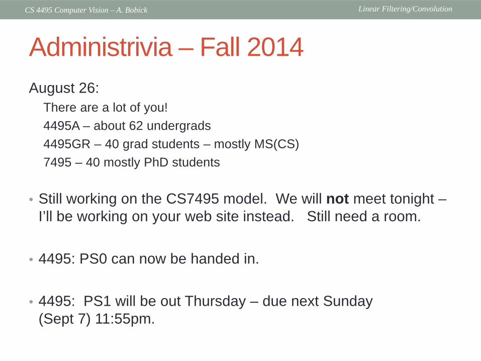
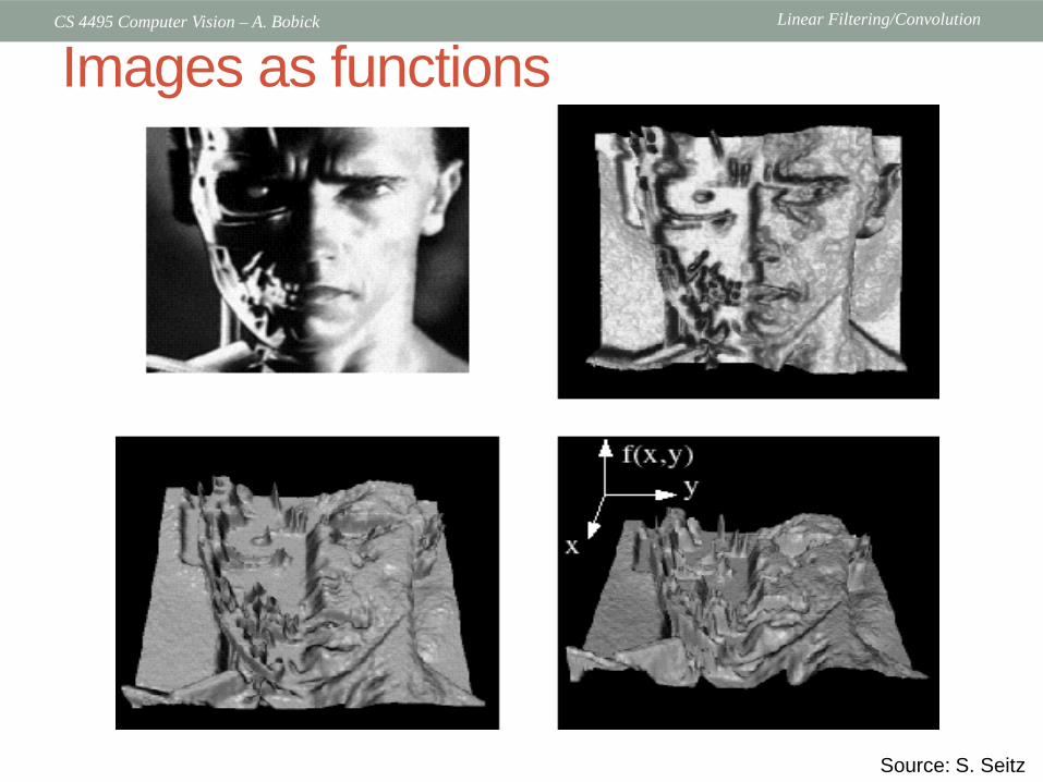
Images as functions
Source: S. Seitz
Linear Filtering/ConvolutionCS 4495 Computer Vision – A. Bobick
Images as functions
Source: S. Seitz
( , )( , ) ( , )
( , )
r x yf x y g x y
b x y
=
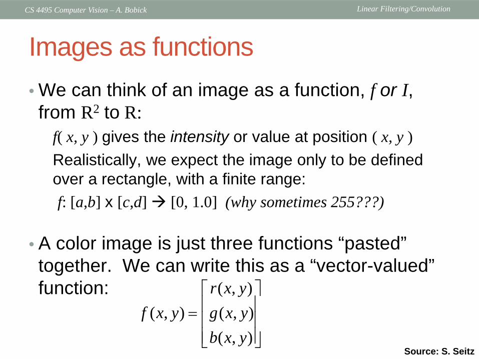
• We can think of an image as a function, f or I, from R2 to R:
f( x, y ) gives the intensity or value at position ( x, y )Realistically, we expect the image only to be defined over a rectangle, with a finite range:f: [a,b] x [c,d] [0, 1.0] (why sometimes 255???)
• A color image is just three functions “pasted” together. We can write this as a “vector-valued” function:
Linear Filtering/ConvolutionCS 4495 Computer Vision – A. Bobick
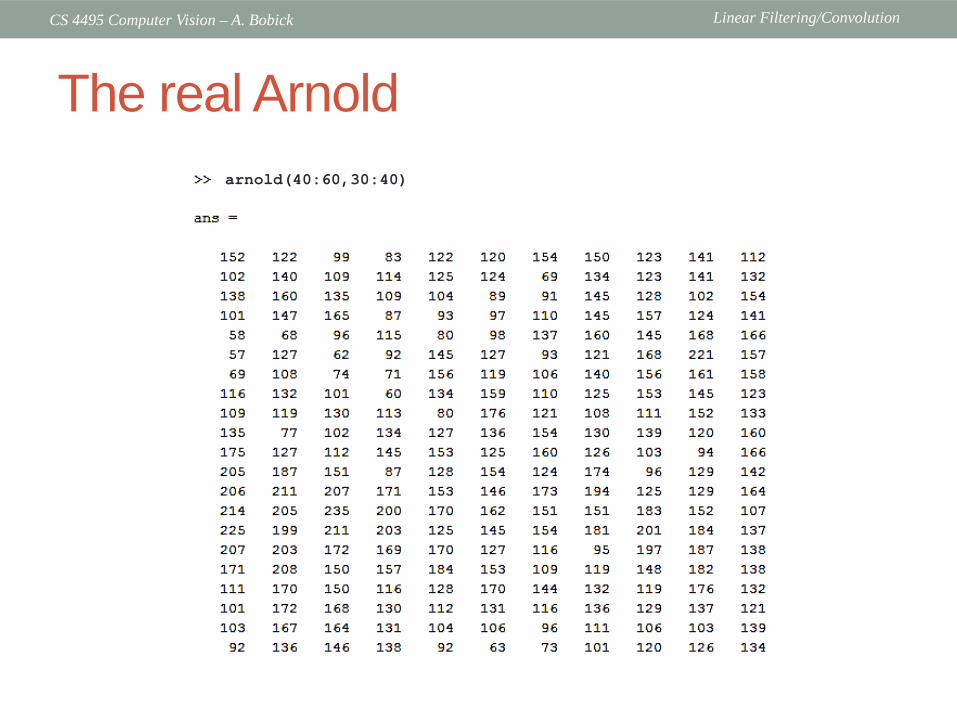
The real Arnoldarnold(40:60,30:40)
Linear Filtering/ConvolutionCS 4495 Computer Vision – A. Bobick
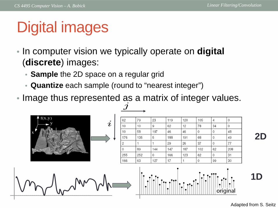
Digital images• In computer vision we typically operate on digital
(discrete) images:• Sample the 2D space on a regular grid• Quantize each sample (round to “nearest integer”)
• Image thus represented as a matrix of integer values.
2D
1D
Adapted from S. Seitz
Linear Filtering/ConvolutionCS 4495 Computer Vision – A. Bobick
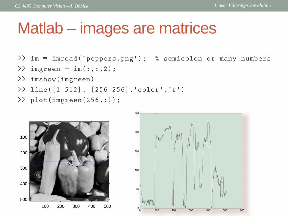
Matlab – images are matrices
>> im = imread('peppers.png'); % semicolon or many numbers
>> imgreen = im(:,:,2);
>> imshow(imgreen)
>> line([1 512], [256 256],'color','r')
>> plot(imgreen(256,:));
100 200 300 400 500
100
200
300
400
500
Linear Filtering/ConvolutionCS 4495 Computer Vision – A. Bobick
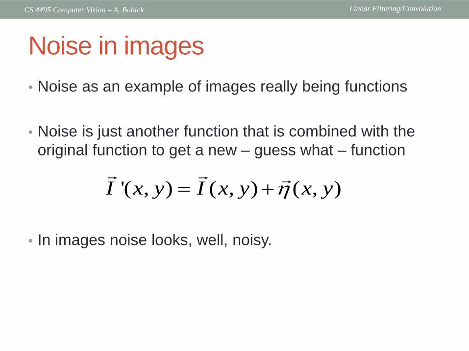
Noise in images• Noise as an example of images really being functions
• Noise is just another function that is combined with the original function to get a new – guess what – function
• In images noise looks, well, noisy.
'( , ) ( , ) ( , )I x y I x y x yη= +

Linear Filtering/ConvolutionCS 4495 Computer Vision – A. Bobick
Common types of noise• Salt and pepper noise:
random occurrences of black and white pixels
• Impulse noise: random occurrences of white pixels
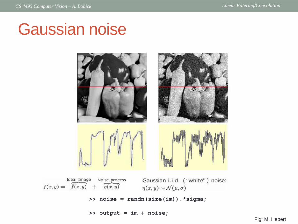
• Gaussian noise: variations in intensity drawn from a Gaussian normal distribution
Source: S. Seitz
Linear Filtering/ConvolutionCS 4495 Computer Vision – A. Bobick
Gaussian noise
Fig: M. Hebert
>> noise = randn(size(im)).*sigma;
>> output = im + noise;
Linear Filtering/ConvolutionCS 4495 Computer Vision – A. Bobick
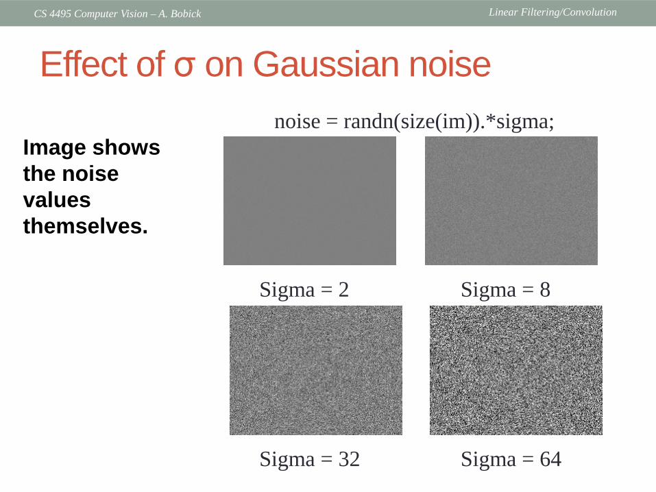
Image shows the noise values themselves.
Sigma = 2 Sigma = 8
Sigma = 32 Sigma = 64
noise = randn(size(im)).*sigma;
Effect of σ on Gaussian noise

Linear Filtering/ConvolutionCS 4495 Computer Vision – A. Bobick
BE VERY CAREFUL!!!• In previous slides, I did not say (at least wasn’t supposed to
say) what the range of the image was. A 𝜎𝜎 of 1.0 would be tiny if the range is [0 255] but huge if [0.0 1.0].
• Matlab can do either and you need to be very careful. If in doubt convert to double.
• Even more difficult can be displaying the image. Things like:• imshow(I,[LOW HIGH])
display the image from [low high]
Don’t worry – you’ll get used to these hassles… see problem set PS0.

Linear Filtering/ConvolutionCS 4495 Computer Vision – A. Bobick
Back to our program…

Linear Filtering/ConvolutionCS 4495 Computer Vision – A. Bobick
Suppose want to remove the noise…

Linear Filtering/ConvolutionCS 4495 Computer Vision – A. Bobick
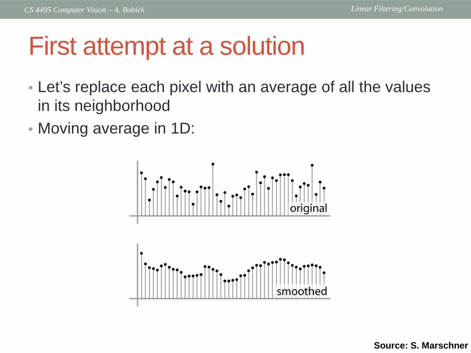
First attempt at a solution• Suggestions? • Let’s replace each pixel with an average of all the values
in its neighborhood• Assumptions:
• Expect pixels to be like their neighbors• Expect noise processes to be independent from pixel to pixel
K. Grauman
Linear Filtering/ConvolutionCS 4495 Computer Vision – A. Bobick
First attempt at a solution• Let’s replace each pixel with an average of all the values
in its neighborhood• Moving average in 1D:
Source: S. Marschner

Linear Filtering/ConvolutionCS 4495 Computer Vision – A. Bobick
Weighted Moving Average• Can add weights to our moving average• Weights [1, 1, 1, 1, 1] / 5
Source: S. Marschner
Linear Filtering/ConvolutionCS 4495 Computer Vision – A. Bobick
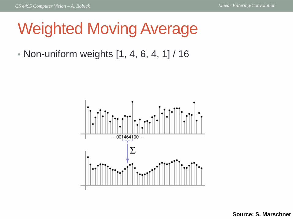
Weighted Moving Average• Non-uniform weights [1, 4, 6, 4, 1] / 16
Source: S. Marschner
Linear Filtering/ConvolutionCS 4495 Computer Vision – A. Bobick
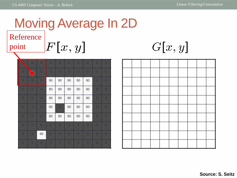
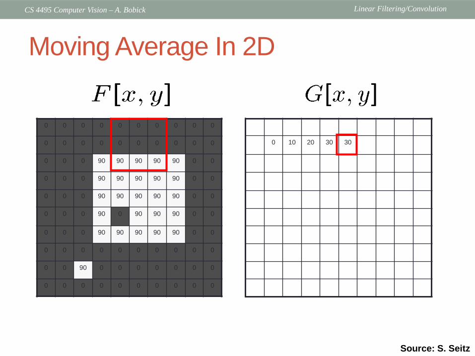
Moving Average In 2D
0 0 0 0 0 0 0 0 0 0
0 0 0 0 0 0 0 0 0 0
0 0 0 90 90 90 90 90 0 0
0 0 0 90 90 90 90 90 0 0
0 0 0 90 90 90 90 90 0 0
0 0 0 90 0 90 90 90 0 0
0 0 0 90 90 90 90 90 0 0
0 0 0 0 0 0 0 0 0 0
0 0 90 0 0 0 0 0 0 0
0 0 0 0 0 0 0 0 0 0
0 0 0 0 0 0 0 0 0 0
0 0 0 0 0 0 0 0 0 0
0 0 0 90 90 90 90 90 0 0
0 0 0 90 90 90 90 90 0 0
0 0 0 90 90 90 90 90 0 0
0 0 0 90 0 90 90 90 0 0
0 0 0 90 90 90 90 90 0 0
0 0 0 0 0 0 0 0 0 0
0 0 90 0 0 0 0 0 0 0
0 0 0 0 0 0 0 0 0 0
Source: S. Seitz
Referencepoint

Linear Filtering/ConvolutionCS 4495 Computer Vision – A. Bobick
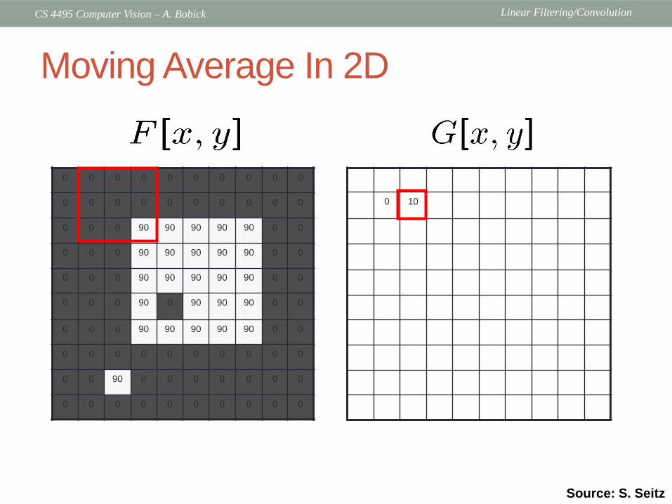
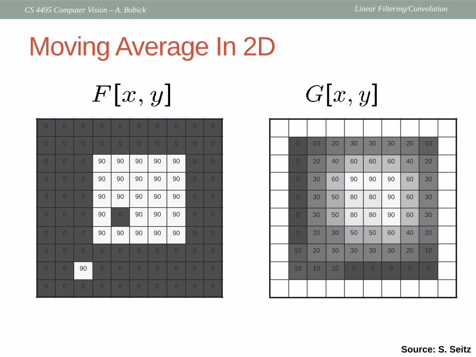
Moving Average In 2D
0 0 0 0 0 0 0 0 0 0
0 0 0 0 0 0 0 0 0 0
0 0 0 90 90 90 90 90 0 0
0 0 0 90 90 90 90 90 0 0
0 0 0 90 90 90 90 90 0 0
0 0 0 90 0 90 90 90 0 0
0 0 0 90 90 90 90 90 0 0
0 0 0 0 0 0 0 0 0 0
0 0 90 0 0 0 0 0 0 0
0 0 0 0 0 0 0 0 0 0
0
0 0 0 0 0 0 0 0 0 0
0 0 0 0 0 0 0 0 0 0
0 0 0 90 90 90 90 90 0 0
0 0 0 90 90 90 90 90 0 0
0 0 0 90 90 90 90 90 0 0
0 0 0 90 0 90 90 90 0 0
0 0 0 90 90 90 90 90 0 0
0 0 0 0 0 0 0 0 0 0
0 0 90 0 0 0 0 0 0 0
0 0 0 0 0 0 0 0 0 0
Source: S. Seitz
Linear Filtering/ConvolutionCS 4495 Computer Vision – A. Bobick
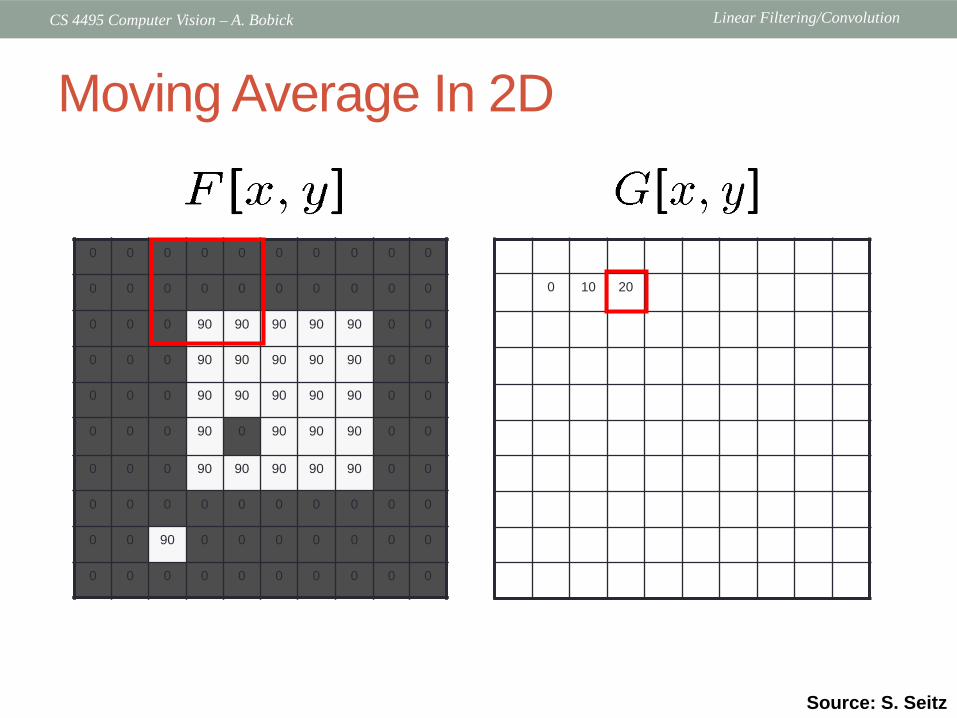
Moving Average In 2D
0 0 0 0 0 0 0 0 0 0
0 0 0 0 0 0 0 0 0 0
0 0 0 90 90 90 90 90 0 0
0 0 0 90 90 90 90 90 0 0
0 0 0 90 90 90 90 90 0 0
0 0 0 90 0 90 90 90 0 0
0 0 0 90 90 90 90 90 0 0
0 0 0 0 0 0 0 0 0 0
0 0 90 0 0 0 0 0 0 0
0 0 0 0 0 0 0 0 0 0
0 10
0 0 0 0 0 0 0 0 0 0
0 0 0 0 0 0 0 0 0 0
0 0 0 90 90 90 90 90 0 0
0 0 0 90 90 90 90 90 0 0
0 0 0 90 90 90 90 90 0 0
0 0 0 90 0 90 90 90 0 0
0 0 0 90 90 90 90 90 0 0
0 0 0 0 0 0 0 0 0 0
0 0 90 0 0 0 0 0 0 0
0 0 0 0 0 0 0 0 0 0
Source: S. Seitz
Linear Filtering/ConvolutionCS 4495 Computer Vision – A. Bobick
Moving Average In 2D
0 0 0 0 0 0 0 0 0 0
0 0 0 0 0 0 0 0 0 0
0 0 0 90 90 90 90 90 0 0
0 0 0 90 90 90 90 90 0 0
0 0 0 90 90 90 90 90 0 0
0 0 0 90 0 90 90 90 0 0
0 0 0 90 90 90 90 90 0 0
0 0 0 0 0 0 0 0 0 0
0 0 90 0 0 0 0 0 0 0
0 0 0 0 0 0 0 0 0 0
0 10 20
0 0 0 0 0 0 0 0 0 0
0 0 0 0 0 0 0 0 0 0
0 0 0 90 90 90 90 90 0 0
0 0 0 90 90 90 90 90 0 0
0 0 0 90 90 90 90 90 0 0
0 0 0 90 0 90 90 90 0 0
0 0 0 90 90 90 90 90 0 0
0 0 0 0 0 0 0 0 0 0
0 0 90 0 0 0 0 0 0 0
0 0 0 0 0 0 0 0 0 0
Source: S. Seitz

Linear Filtering/ConvolutionCS 4495 Computer Vision – A. Bobick
Moving Average In 2D
0 0 0 0 0 0 0 0 0 0
0 0 0 0 0 0 0 0 0 0
0 0 0 90 90 90 90 90 0 0
0 0 0 90 90 90 90 90 0 0
0 0 0 90 90 90 90 90 0 0
0 0 0 90 0 90 90 90 0 0
0 0 0 90 90 90 90 90 0 0
0 0 0 0 0 0 0 0 0 0
0 0 90 0 0 0 0 0 0 0
0 0 0 0 0 0 0 0 0 0
0 10 20 30
0 0 0 0 0 0 0 0 0 0
0 0 0 0 0 0 0 0 0 0
0 0 0 90 90 90 90 90 0 0
0 0 0 90 90 90 90 90 0 0
0 0 0 90 90 90 90 90 0 0
0 0 0 90 0 90 90 90 0 0
0 0 0 90 90 90 90 90 0 0
0 0 0 0 0 0 0 0 0 0
0 0 90 0 0 0 0 0 0 0
0 0 0 0 0 0 0 0 0 0
Source: S. Seitz
Linear Filtering/ConvolutionCS 4495 Computer Vision – A. Bobick
Moving Average In 2D
0 10 20 30 30
0 0 0 0 0 0 0 0 0 0
0 0 0 0 0 0 0 0 0 0
0 0 0 90 90 90 90 90 0 0
0 0 0 90 90 90 90 90 0 0
0 0 0 90 90 90 90 90 0 0
0 0 0 90 0 90 90 90 0 0
0 0 0 90 90 90 90 90 0 0
0 0 0 0 0 0 0 0 0 0
0 0 90 0 0 0 0 0 0 0
0 0 0 0 0 0 0 0 0 0
Source: S. Seitz
Linear Filtering/ConvolutionCS 4495 Computer Vision – A. Bobick
Moving Average In 2D
0 10 20 30 30 30 20 10
0 20 40 60 60 60 40 20
0 30 60 90 90 90 60 30
0 30 50 80 80 90 60 30
0 30 50 80 80 90 60 30
0 20 30 50 50 60 40 20
10 20 30 30 30 30 20 10
10 10 10 0 0 0 0 0
0 0 0 0 0 0 0 0 0 0
0 0 0 0 0 0 0 0 0 0
0 0 0 90 90 90 90 90 0 0
0 0 0 90 90 90 90 90 0 0
0 0 0 90 90 90 90 90 0 0
0 0 0 90 0 90 90 90 0 0
0 0 0 90 90 90 90 90 0 0
0 0 0 0 0 0 0 0 0 0
0 0 90 0 0 0 0 0 0 0
0 0 0 0 0 0 0 0 0 0
Source: S. Seitz
Linear Filtering/ConvolutionCS 4495 Computer Vision – A. Bobick
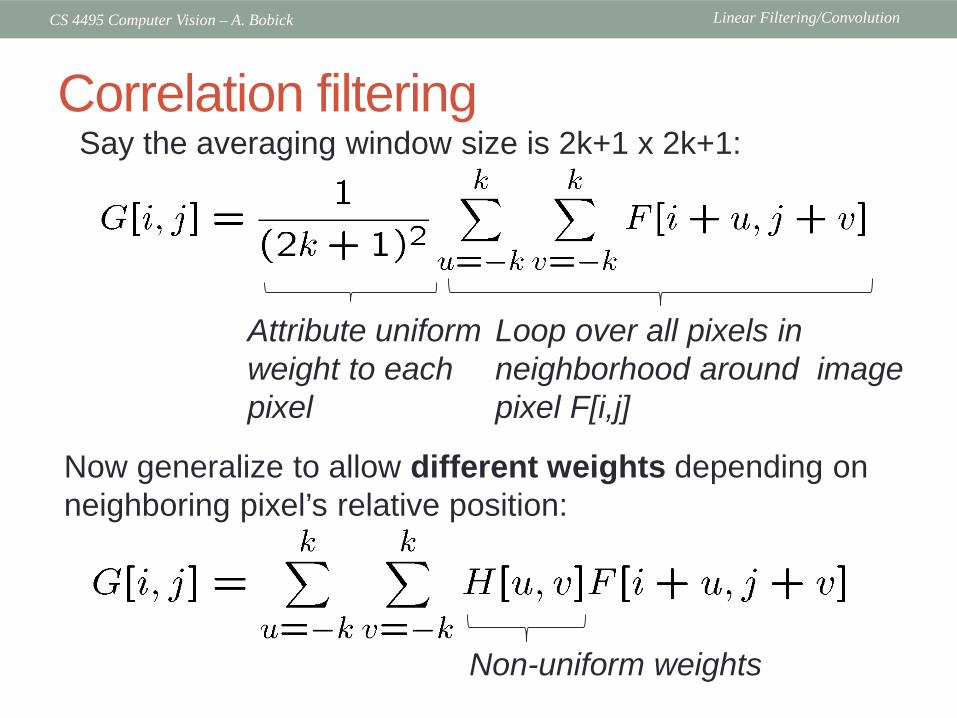
Correlation filteringSay the averaging window size is 2k+1 x 2k+1:
Loop over all pixels in neighborhood around image pixel F[i,j]
Attribute uniform weight to each pixel
Now generalize to allow different weights depending on neighboring pixel’s relative position:
Non-uniform weights

Linear Filtering/ConvolutionCS 4495 Computer Vision – A. Bobick
Correlation filtering
Filtering an image: replace each pixel with a linear combination of its neighbors.
The filter “kernel” or “mask” H[u,v] is the prescription for the weights in the linear combination.
This is called cross-correlation, denoted
Linear Filtering/ConvolutionCS 4495 Computer Vision – A. Bobick
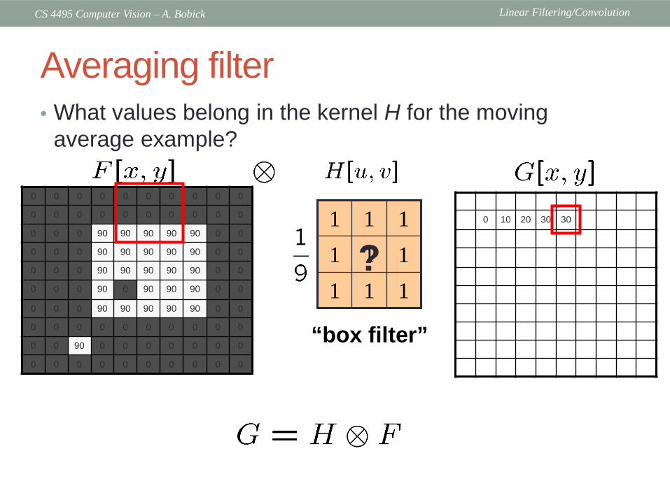
Averaging filter• What values belong in the kernel H for the moving
average example?
0 10 20 30 30
0 0 0 0 0 0 0 0 0 0
0 0 0 0 0 0 0 0 0 0
0 0 0 90 90 90 90 90 0 0
0 0 0 90 90 90 90 90 0 0
0 0 0 90 90 90 90 90 0 0
0 0 0 90 0 90 90 90 0 0
0 0 0 90 90 90 90 90 0 0
0 0 0 0 0 0 0 0 0 0
0 0 90 0 0 0 0 0 0 0
0 0 0 0 0 0 0 0 0 0
111111111
“box filter”
?
Linear Filtering/ConvolutionCS 4495 Computer Vision – A. Bobick
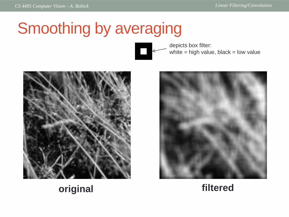
Smoothing by averagingdepicts box filter: white = high value, black = low value
original filtered

Linear Filtering/ConvolutionCS 4495 Computer Vision – A. Bobick
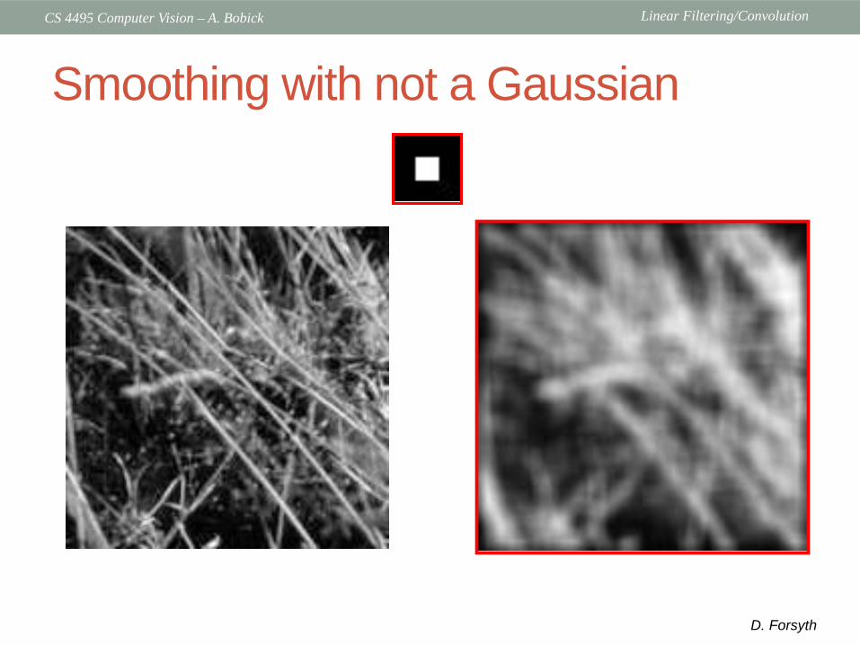
Squares aren’t smooth…
• Smoothing with an average actually doesn’t compare at all well with a defocussed lens
• Most obvious difference is that a single point of light viewed in a defocussed lens looks like a fuzzy blob; but the averaging process would give a little square.
• More about “impulse” responses later…
D. Forsyth
Linear Filtering/ConvolutionCS 4495 Computer Vision – A. Bobick
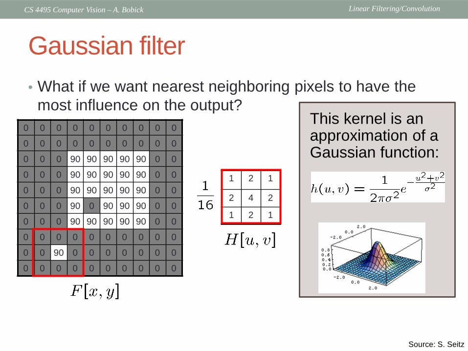
Gaussian filter• What if we want nearest neighboring pixels to have the
most influence on the output?0 0 0 0 0 0 0 0 0 0
0 0 0 0 0 0 0 0 0 0
0 0 0 90 90 90 90 90 0 0
0 0 0 90 90 90 90 90 0 0
0 0 0 90 90 90 90 90 0 0
0 0 0 90 0 90 90 90 0 0
0 0 0 90 90 90 90 90 0 0
0 0 0 0 0 0 0 0 0 0
0 0 90 0 0 0 0 0 0 0
0 0 0 0 0 0 0 0 0 0
1 2 1
2 4 2
1 2 1
This kernel is an approximation of a Gaussian function:
Source: S. Seitz

Linear Filtering/ConvolutionCS 4495 Computer Vision – A. Bobick
The picture shows a smoothing kernel proportional to
(which is a reasonable model of a circularly symmetric fuzzy blob)
An Isotropic Gaussian
D. Forsyth
2 2
2e ( )2
x ( )p x xσ+
−
Linear Filtering/ConvolutionCS 4495 Computer Vision – A. Bobick
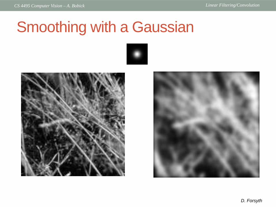
Smoothing with a Gaussian
D. Forsyth
Linear Filtering/ConvolutionCS 4495 Computer Vision – A. Bobick
Smoothing with not a Gaussian
D. Forsyth
Linear Filtering/ConvolutionCS 4495 Computer Vision – A. Bobick
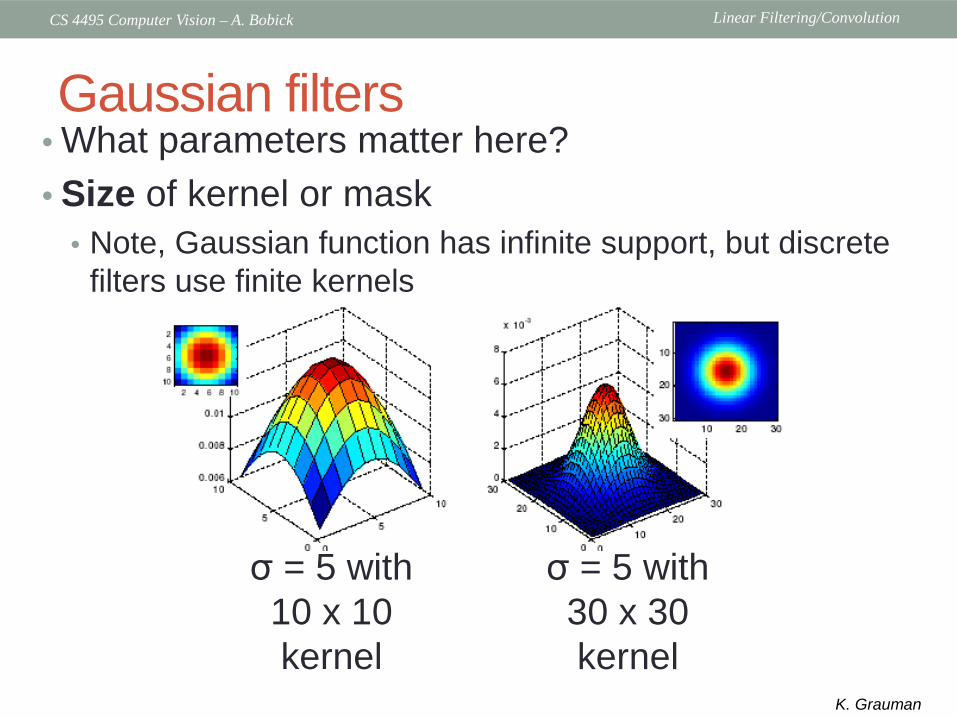
Gaussian filters• What parameters matter here?• Size of kernel or mask
• Note, Gaussian function has infinite support, but discrete filters use finite kernels
σ = 5 with 10 x 10 kernel
σ = 5 with 30 x 30 kernel
K. Grauman

Linear Filtering/ConvolutionCS 4495 Computer Vision – A. Bobick
Gaussian filters• What parameters matter here?• Variance of Gaussian: determines extent of smoothing
σ = 2 with 30 x 30 kernel
σ = 5 with 30 x 30 kernel
K. Grauman
Linear Filtering/ConvolutionCS 4495 Computer Vision – A. Bobick
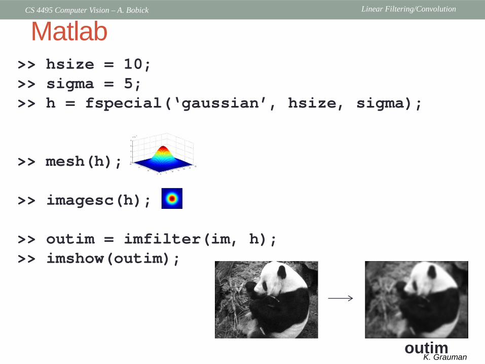
Matlab>> hsize = 10;>> sigma = 5;>> h = fspecial(‘gaussian’, hsize, sigma);
>> mesh(h);
>> imagesc(h);
>> outim = imfilter(im, h);>> imshow(outim);
outimK. Grauman
Linear Filtering/ConvolutionCS 4495 Computer Vision – A. Bobick
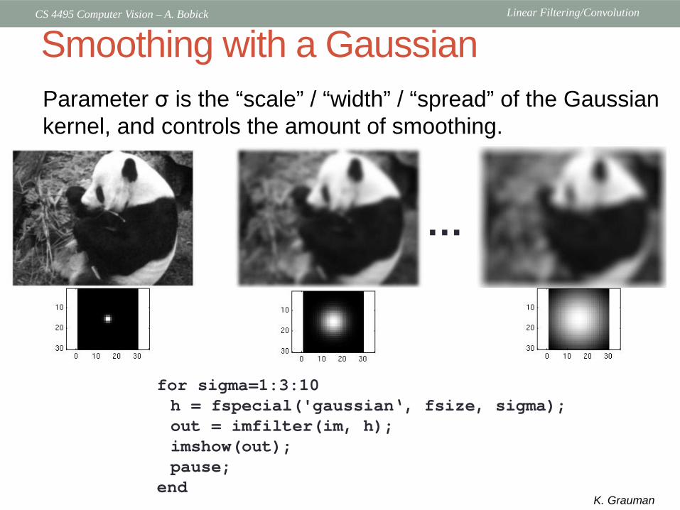
Smoothing with a Gaussian
for sigma=1:3:10 h = fspecial('gaussian‘, fsize, sigma);out = imfilter(im, h); imshow(out);pause;
end
…
Parameter σ is the “scale” / “width” / “spread” of the Gaussian kernel, and controls the amount of smoothing.
K. Grauman
Linear Filtering/ConvolutionCS 4495 Computer Vision – A. Bobick
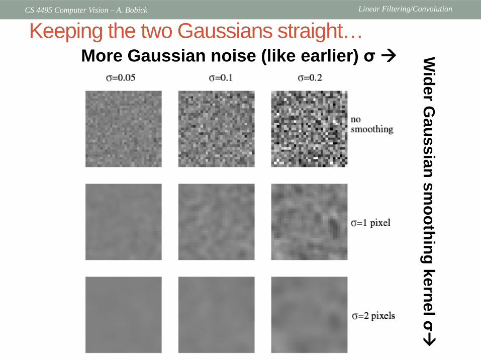
More Gaussian noise (like earlier) σ Wider G
aussian smoothing kernel σ
Keeping the two Gaussians straight…
Linear Filtering/ConvolutionCS 4495 Computer Vision – A. Bobick
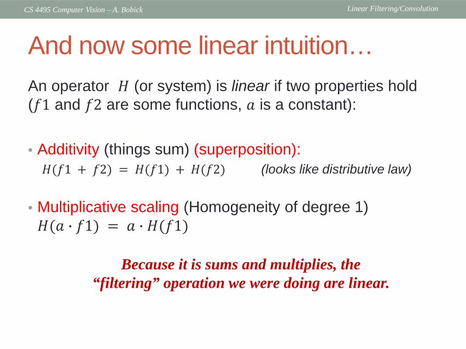
And now some linear intuition…An operator 𝐻𝐻 (or system) is linear if two properties hold (𝑓𝑓𝑓 and 𝑓𝑓𝑓 are some functions, 𝑎𝑎 is a constant):
• Additivity (things sum) (superposition):𝐻𝐻(𝑓𝑓𝑓 + 𝑓𝑓𝑓) = 𝐻𝐻(𝑓𝑓𝑓) + 𝐻𝐻(𝑓𝑓𝑓) (looks like distributive law)
• Multiplicative scaling (Homogeneity of degree 1)𝐻𝐻(𝑎𝑎 � 𝑓𝑓𝑓) = 𝑎𝑎 � 𝐻𝐻(𝑓𝑓𝑓)
Because it is sums and multiplies, the “filtering” operation we were doing are linear.

Linear Filtering/ConvolutionCS 4495 Computer Vision – A. Bobick
An impulse function…• In the discrete world, and impulse is a very easy signal to
understand: it’s just a value of 1 at a single location.
• In the continuous world, an impulse is an idealized function that is very narrow and very tall so that it has a unit area. In the limit:
1.0
Area = 1.0
Linear Filtering/ConvolutionCS 4495 Computer Vision – A. Bobick
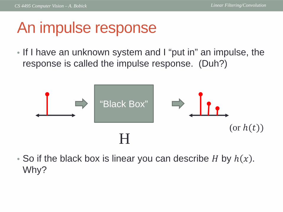
An impulse response• If I have an unknown system and I “put in” an impulse, the
response is called the impulse response. (Duh?)
• So if the black box is linear you can describe 𝐻𝐻 by ℎ 𝑥𝑥 .Why?
“Black Box”
H(or ℎ(𝑡𝑡))
Linear Filtering/ConvolutionCS 4495 Computer Vision – A. Bobick
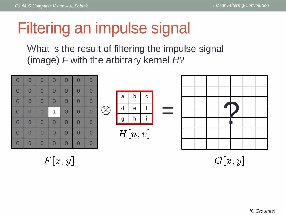
Filtering an impulse signal
0 0 0 0 0 0 0
0 0 0 0 0 0 0
0 0 0 0 0 0 0
0 0 0 1 0 0 0
0 0 0 0 0 0 0
0 0 0 0 0 0 0
0 0 0 0 0 0 0
a b c
d e f
g h i
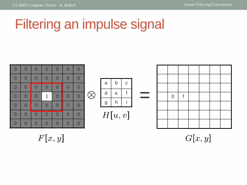
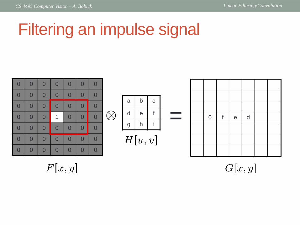
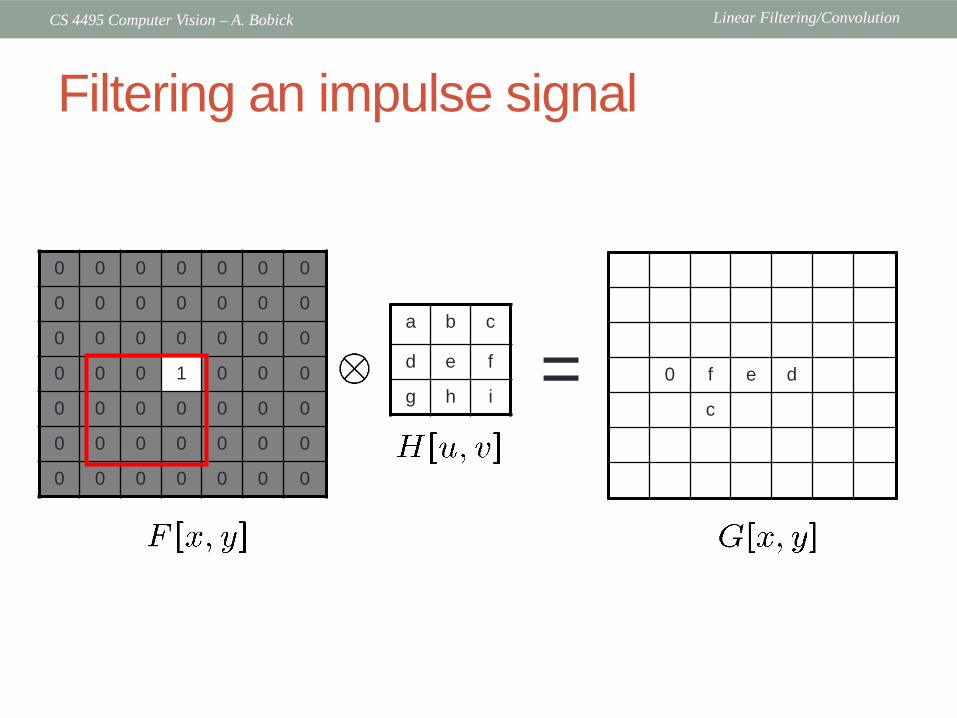
What is the result of filtering the impulse signal (image) F with the arbitrary kernel H?
?
K. Grauman
=

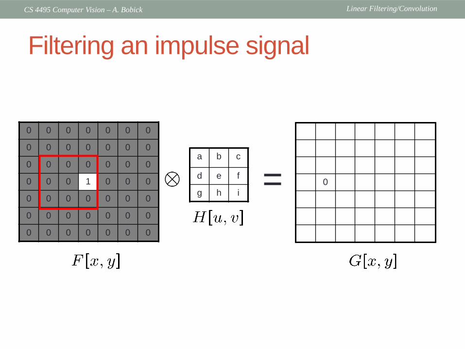
Linear Filtering/ConvolutionCS 4495 Computer Vision – A. Bobick
Filtering an impulse signal
0 0 0 0 0 0 0
0 0 0 0 0 0 0
0 0 0 0 0 0 0
0 0 0 1 0 0 0
0 0 0 0 0 0 0
0 0 0 0 0 0 0
0 0 0 0 0 0 0
a b c
d e f
g h i0=
Linear Filtering/ConvolutionCS 4495 Computer Vision – A. Bobick
Filtering an impulse signal
0 0 0 0 0 0 0
0 0 0 0 0 0 0
0 0 0 0 0 0 0
0 0 0 1 0 0 0
0 0 0 0 0 0 0
0 0 0 0 0 0 0
0 0 0 0 0 0 0
a b c
d e f
g h i0=

Linear Filtering/ConvolutionCS 4495 Computer Vision – A. Bobick
Filtering an impulse signal
0 0 0 0 0 0 0
0 0 0 0 0 0 0
0 0 0 0 0 0 0
0 0 0 1 0 0 0
0 0 0 0 0 0 0
0 0 0 0 0 0 0
0 0 0 0 0 0 0
a b c
d e f
g h i0 f=
Linear Filtering/ConvolutionCS 4495 Computer Vision – A. Bobick
Filtering an impulse signal
0 0 0 0 0 0 0
0 0 0 0 0 0 0
0 0 0 0 0 0 0
0 0 0 1 0 0 0
0 0 0 0 0 0 0
0 0 0 0 0 0 0
0 0 0 0 0 0 0
a b c
d e f
g h i0 f=

Linear Filtering/ConvolutionCS 4495 Computer Vision – A. Bobick
Filtering an impulse signal
0 0 0 0 0 0 0
0 0 0 0 0 0 0
0 0 0 0 0 0 0
0 0 0 1 0 0 0
0 0 0 0 0 0 0
0 0 0 0 0 0 0
0 0 0 0 0 0 0
a b c
d e f
g h i0 f e=

Linear Filtering/ConvolutionCS 4495 Computer Vision – A. Bobick
Filtering an impulse signal
0 0 0 0 0 0 0
0 0 0 0 0 0 0
0 0 0 0 0 0 0
0 0 0 1 0 0 0
0 0 0 0 0 0 0
0 0 0 0 0 0 0
0 0 0 0 0 0 0
a b c
d e f
g h i0 f e d=
Linear Filtering/ConvolutionCS 4495 Computer Vision – A. Bobick
Filtering an impulse signal
0 0 0 0 0 0 0
0 0 0 0 0 0 0
0 0 0 0 0 0 0
0 0 0 1 0 0 0
0 0 0 0 0 0 0
0 0 0 0 0 0 0
0 0 0 0 0 0 0
a b c
d e f
g h i0 f e d=

Linear Filtering/ConvolutionCS 4495 Computer Vision – A. Bobick
Filtering an impulse signal
0 0 0 0 0 0 0
0 0 0 0 0 0 0
0 0 0 0 0 0 0
0 0 0 1 0 0 0
0 0 0 0 0 0 0
0 0 0 0 0 0 0
0 0 0 0 0 0 0
a b c
d e f
g h i0 f e d
c=
Linear Filtering/ConvolutionCS 4495 Computer Vision – A. Bobick
Filtering an impulse signal
0 0 0 0 0 0 0
0 0 0 0 0 0 0
0 0 0 0 0 0 0
0 0 0 1 0 0 0
0 0 0 0 0 0 0
0 0 0 0 0 0 0
0 0 0 0 0 0 0
a b c
d e f
g h i0 f e d
c=
Linear Filtering/ConvolutionCS 4495 Computer Vision – A. Bobick
“Filtering” an impulse signal
0 0 0 0 0 0 0
0 0 0 0 0 0 0
0 0 0 0 0 0 0
0 0 0 1 0 0 0
0 0 0 0 0 0 0
0 0 0 0 0 0 0
0 0 0 0 0 0 0
a b c
d e f
g h i
i h g
f e d
c b a
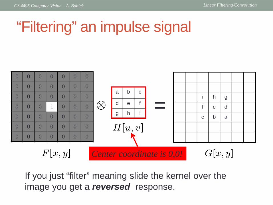
If you just “filter” meaning slide the kernel over the image you get a reversed response.
=
Center coordinate is 0,0!
Linear Filtering/ConvolutionCS 4495 Computer Vision – A. Bobick
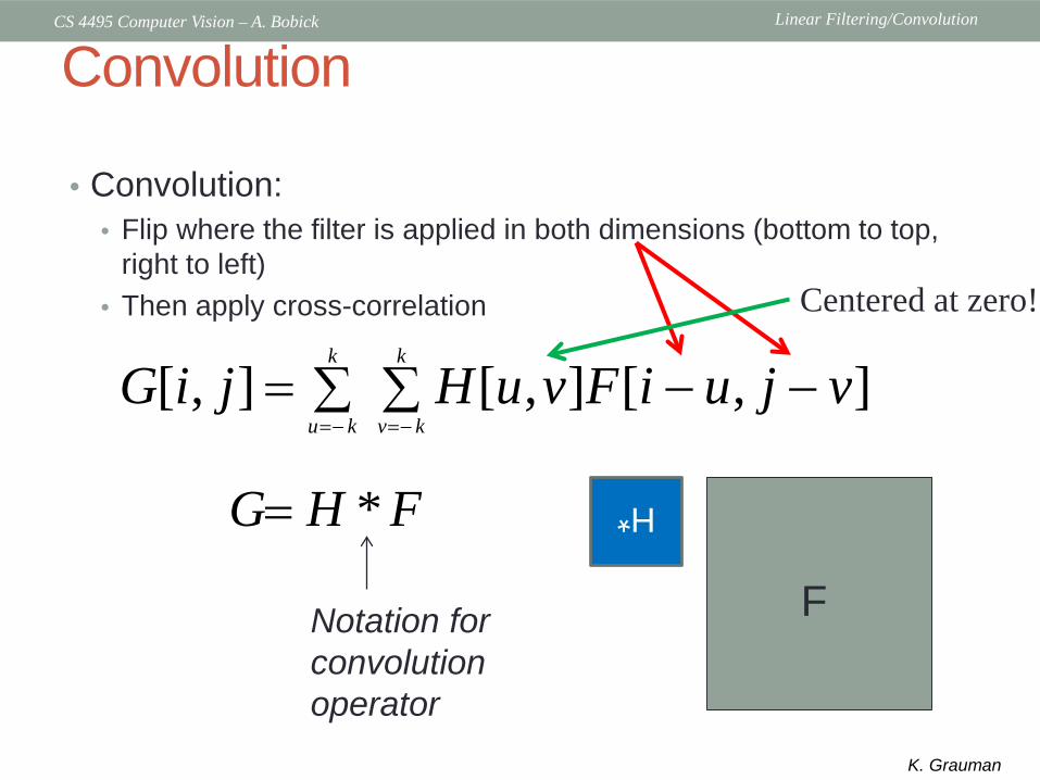
Convolution
• Convolution: • Flip where the filter is applied in both dimensions (bottom to top,
right to left)• Then apply cross-correlation
Notation for convolution operator
H*
F
K. Grauman
H**G H F=
[ , ] [ , ] [ , ]k k
u k v kH u v F iG i u j vj
=− =−− −∑ ∑=
Centered at zero!
Linear Filtering/ConvolutionCS 4495 Computer Vision – A. Bobick
One more thing…• Shift invariant:
• Operator behaves the same everywhere, i.e. the value of the output depends on the pattern in the image neighborhood, not the position of the neighborhood.
Linear Filtering/ConvolutionCS 4495 Computer Vision – A. Bobick
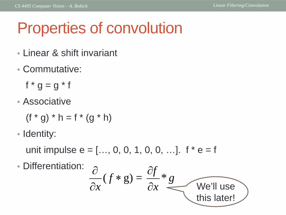
Properties of convolution• Linear & shift invariant
• Commutative:
f * g = g * f
• Associative
(f * g) * h = f * (g * h)
• Identity:
unit impulse e = […, 0, 0, 1, 0, 0, …]. f * e = f
• Differentiation:
We’ll use this later!
g) = ( *ff gx x∂ ∂
∂∗
∂

Linear Filtering/ConvolutionCS 4495 Computer Vision – A. Bobick
Convolution vs. correlationConvolution
Cross-correlation
For a Gaussian or box filter, how will the outputs differ?If the input is an impulse signal, how will the outputs differ?
K. Grauman
Linear Filtering/ConvolutionCS 4495 Computer Vision – A. Bobick
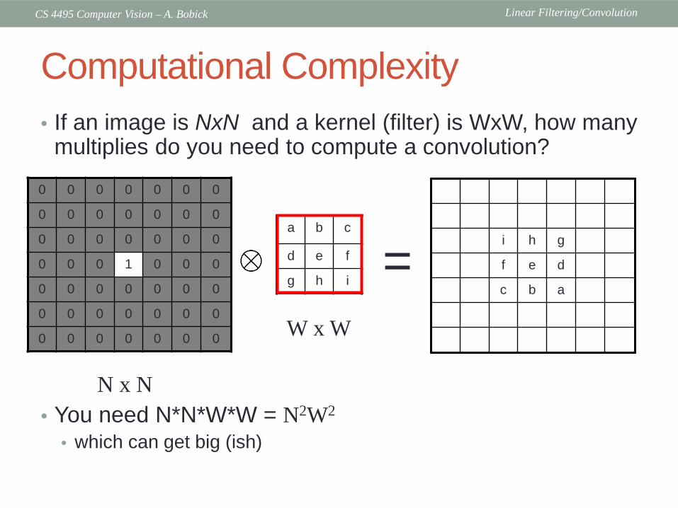
Computational Complexity • If an image is NxN and a kernel (filter) is WxW, how many
multiplies do you need to compute a convolution?
• You need N*N*W*W = N2W2
• which can get big (ish)
0 0 0 0 0 0 0
0 0 0 0 0 0 0
0 0 0 0 0 0 0
0 0 0 1 0 0 0
0 0 0 0 0 0 0
0 0 0 0 0 0 0
0 0 0 0 0 0 0
a b c
d e f
g h i
i h g
f e d
c b a=
N x N
W x W
Linear Filtering/ConvolutionCS 4495 Computer Vision – A. Bobick
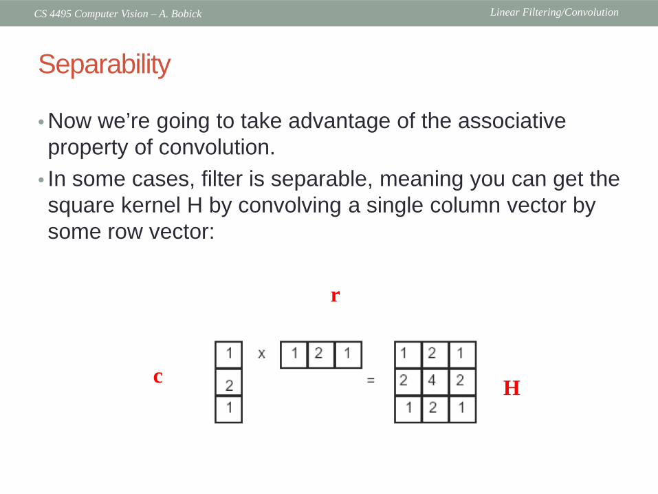
Separability
• Now we’re going to take advantage of the associative property of convolution.
• In some cases, filter is separable, meaning you can get the square kernel H by convolving a single column vector by some row vector:
c
r
H
Linear Filtering/ConvolutionCS 4495 Computer Vision – A. Bobick
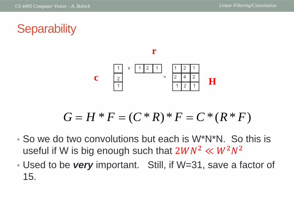
Separability
• So we do two convolutions but each is W*N*N. So this is useful if W is big enough such that 𝑓𝑊𝑊𝑁𝑁2 ≪ 𝑊𝑊2𝑁𝑁2
• Used to be very important. Still, if W=31, save a factor of 15.
* ( * ) * * ( * )G H F C R F C R F= = =
c
r
H
Linear Filtering/ConvolutionCS 4495 Computer Vision – A. Bobick
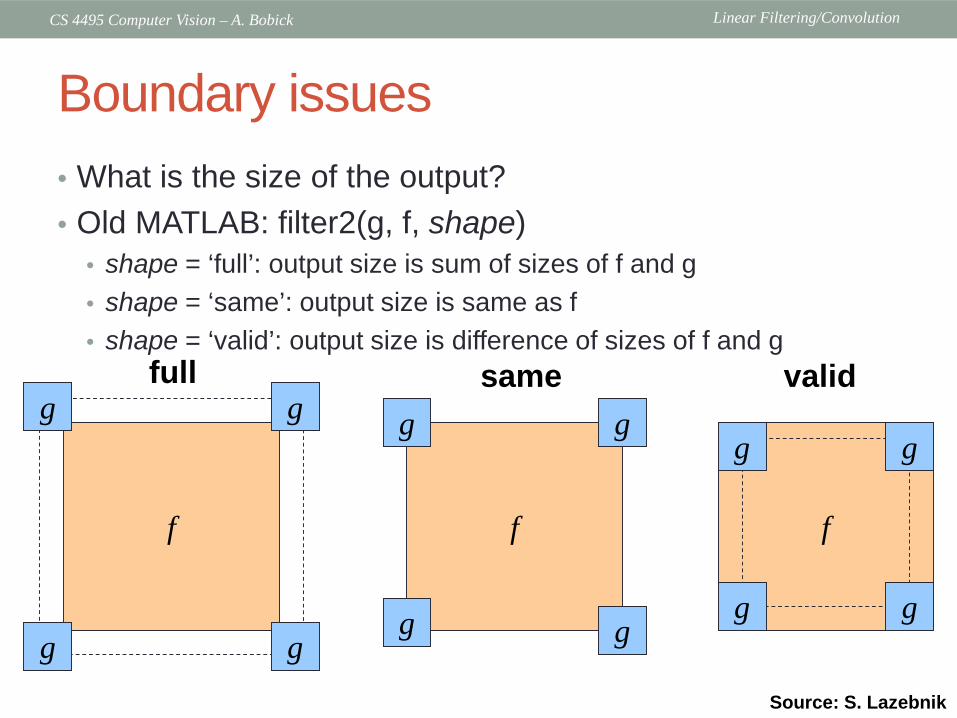
Boundary issues• What is the size of the output?• Old MATLAB: filter2(g, f, shape)
• shape = ‘full’: output size is sum of sizes of f and g• shape = ‘same’: output size is same as f• shape = ‘valid’: output size is difference of sizes of f and g
f
gg
gg
f
gg
gg
f
gg
gg
full same valid
Source: S. Lazebnik
Linear Filtering/ConvolutionCS 4495 Computer Vision – A. Bobick
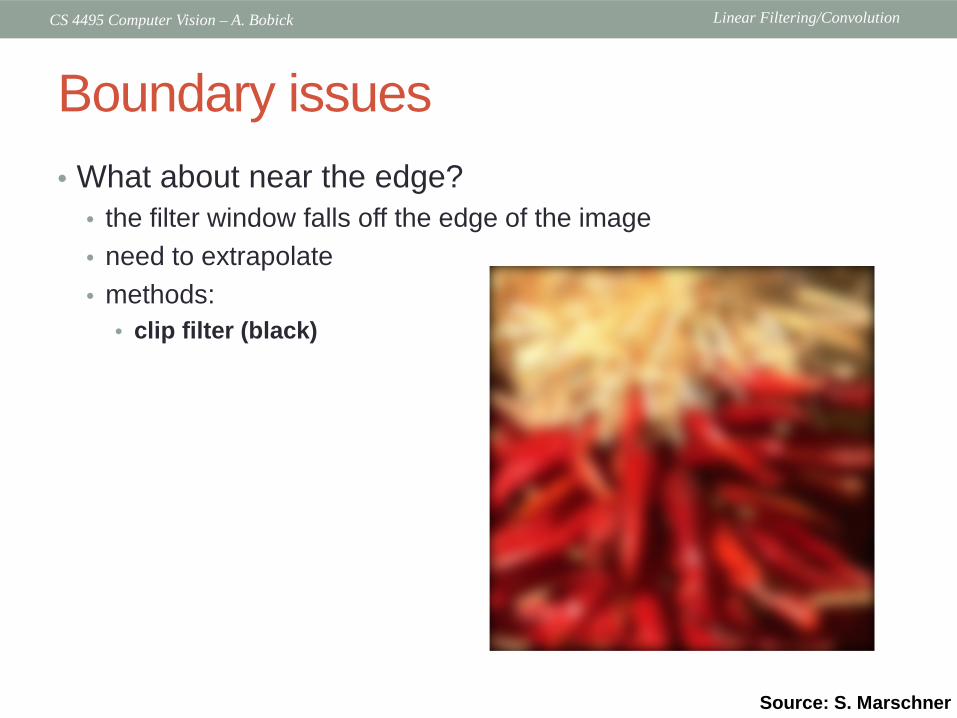
Boundary issues• What about near the edge?
• the filter window falls off the edge of the image• need to extrapolate• methods:
• clip filter (black)
Source: S. Marschner

Linear Filtering/ConvolutionCS 4495 Computer Vision – A. Bobick
Boundary issues• What about near the edge?
• the filter window falls off the edge of the image• need to extrapolate• methods:
• clip filter (black)• wrap around
Source: S. Marschner
Linear Filtering/ConvolutionCS 4495 Computer Vision – A. Bobick
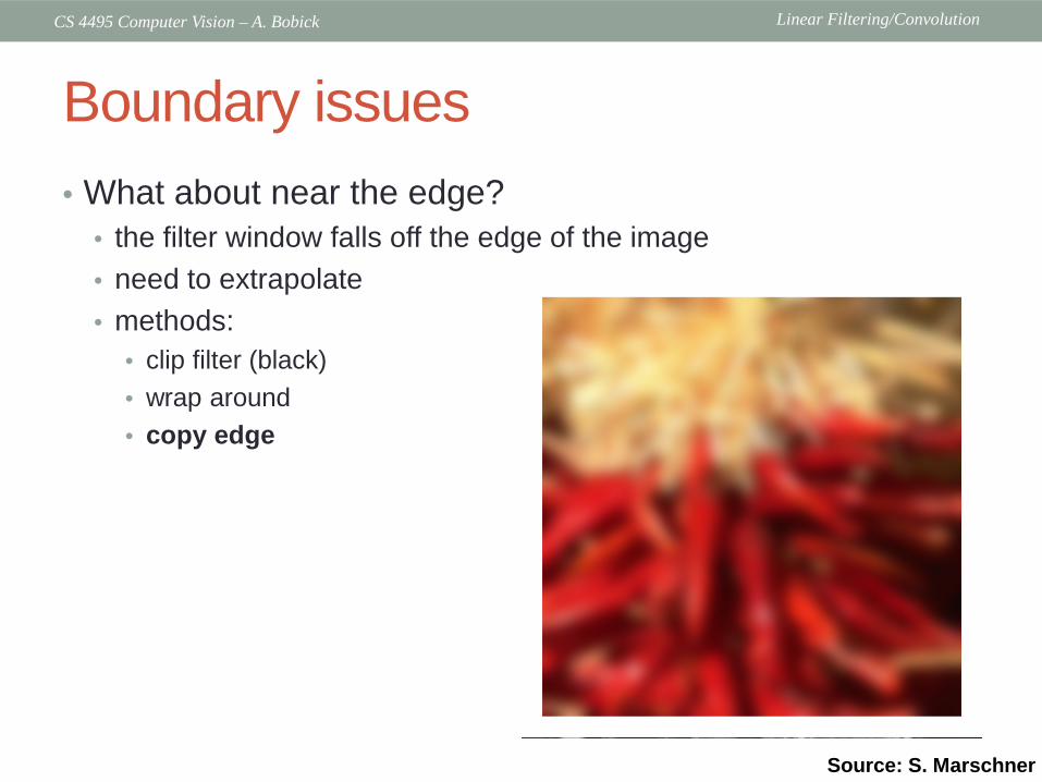
Boundary issues• What about near the edge?
• the filter window falls off the edge of the image• need to extrapolate• methods:
• clip filter (black)• wrap around• copy edge
Source: S. Marschner

Linear Filtering/ConvolutionCS 4495 Computer Vision – A. Bobick
Boundary issues• What about near the edge?
• the filter window falls off the edge of the image• need to extrapolate• methods:
• clip filter (black)• wrap around• copy edge• reflect across edge
Source: S. Marschner
Linear Filtering/ConvolutionCS 4495 Computer Vision – A. Bobick
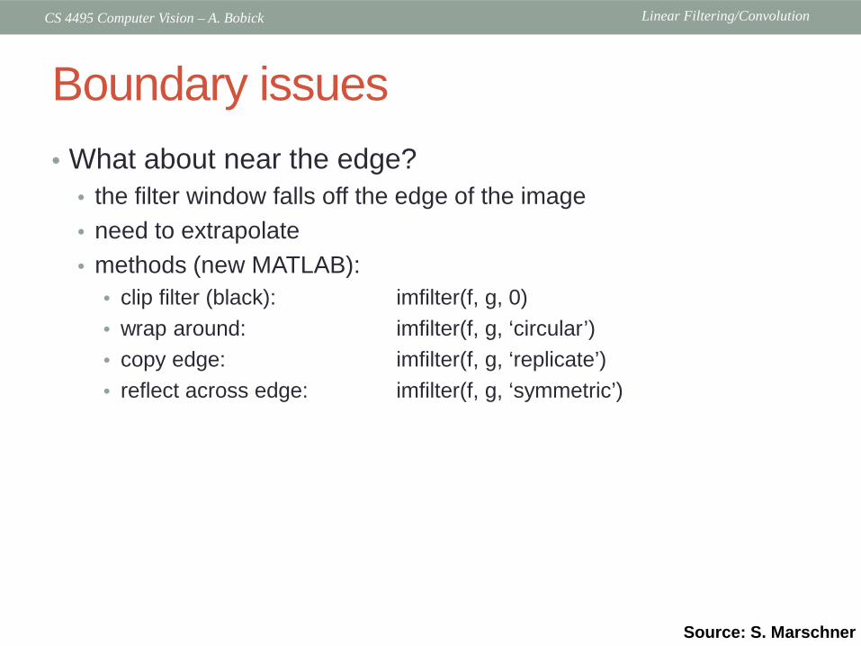
Boundary issues• What about near the edge?
• the filter window falls off the edge of the image• need to extrapolate• methods (new MATLAB):
• clip filter (black): imfilter(f, g, 0)• wrap around: imfilter(f, g, ‘circular’)• copy edge: imfilter(f, g, ‘replicate’)• reflect across edge: imfilter(f, g, ‘symmetric’)
Source: S. Marschner
Linear Filtering/ConvolutionCS 4495 Computer Vision – A. Bobick
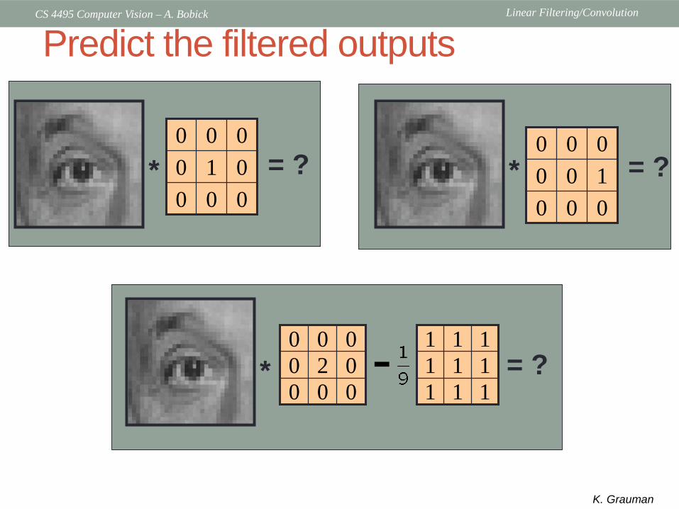
Predict the filtered outputs
000010000
* = ?000100000
* = ?
111111111
000020000 -* = ?
K. Grauman

Linear Filtering/ConvolutionCS 4495 Computer Vision – A. Bobick
Practice with linear filters
000010000
Original
?
Source: D. Lowe

Linear Filtering/ConvolutionCS 4495 Computer Vision – A. Bobick
Practice with linear filters
000010000
Original Filtered (no change)
Source: D. Lowe
Linear Filtering/ConvolutionCS 4495 Computer Vision – A. Bobick
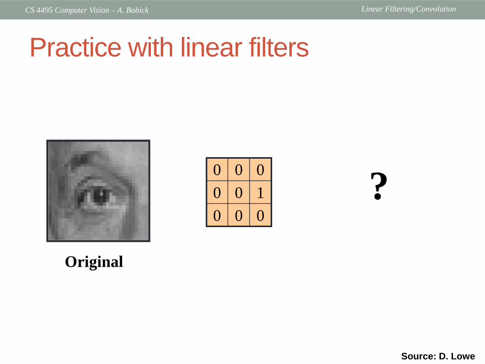
Practice with linear filters
000100000
Original
?
Source: D. Lowe
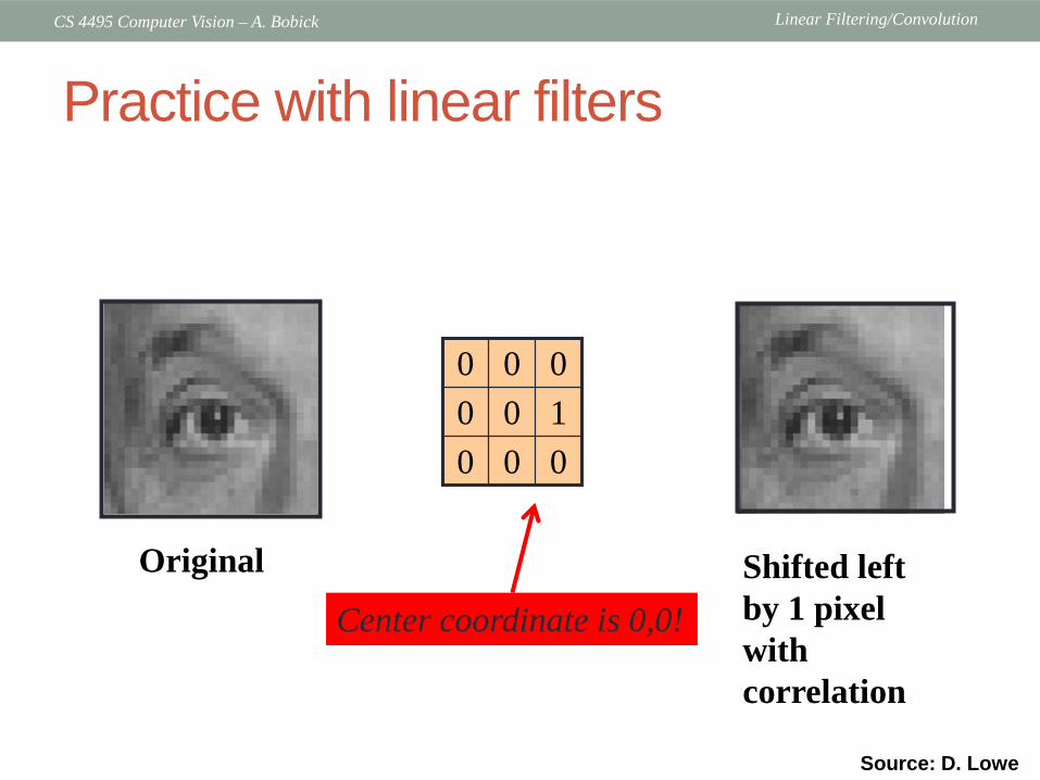
Linear Filtering/ConvolutionCS 4495 Computer Vision – A. Bobick
Practice with linear filters
000100000
Original Shifted leftby 1 pixel with correlation
Source: D. Lowe
Center coordinate is 0,0!
Linear Filtering/ConvolutionCS 4495 Computer Vision – A. Bobick
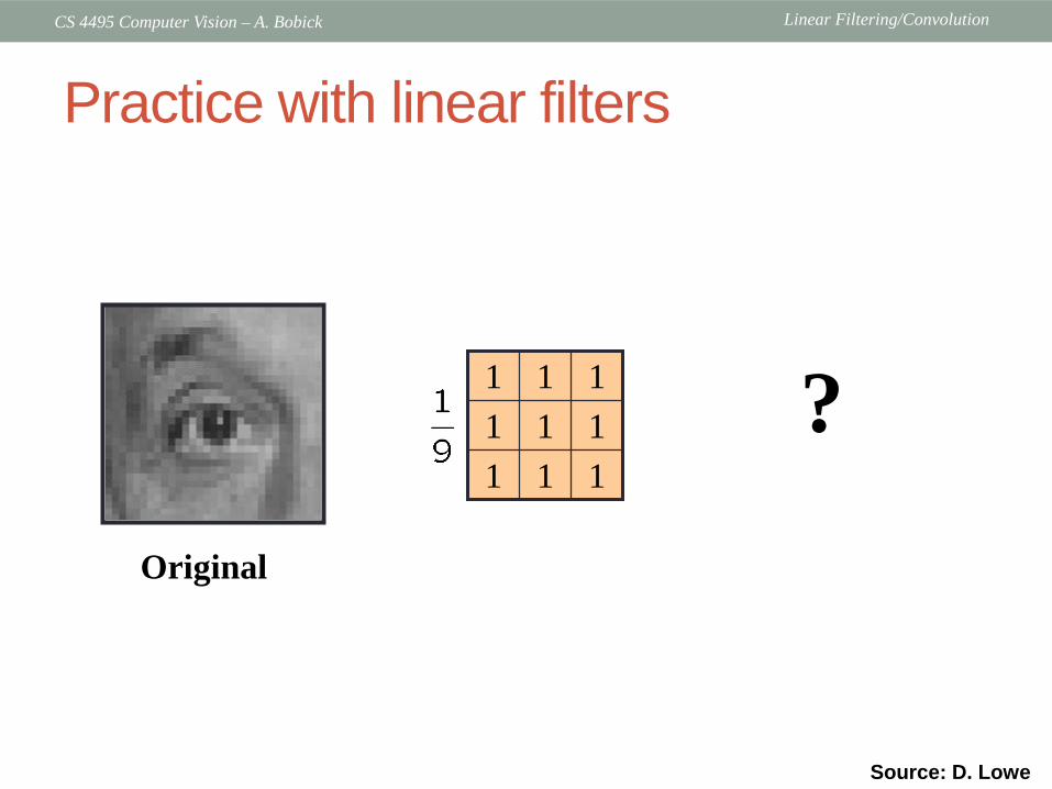
Practice with linear filters
Original
?111111111
Source: D. Lowe
Linear Filtering/ConvolutionCS 4495 Computer Vision – A. Bobick
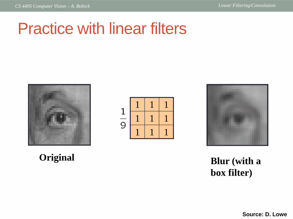
Practice with linear filters
Original
111111111
Blur (with abox filter)
Source: D. Lowe

Linear Filtering/ConvolutionCS 4495 Computer Vision – A. Bobick
Practice with linear filters
Original
111111111
000020000 - ?
Source: D. Lowe
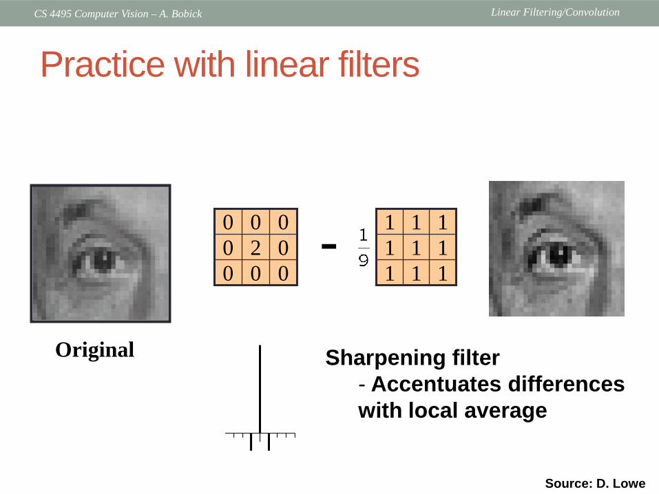
Linear Filtering/ConvolutionCS 4495 Computer Vision – A. Bobick
Practice with linear filters
Original
111111111
000020000 -
Sharpening filter- Accentuates differences with local average
Source: D. Lowe
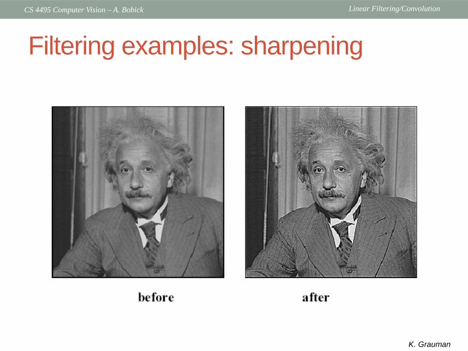
Linear Filtering/ConvolutionCS 4495 Computer Vision – A. Bobick
Filtering examples: sharpening
K. Grauman
Linear Filtering/ConvolutionCS 4495 Computer Vision – A. Bobick
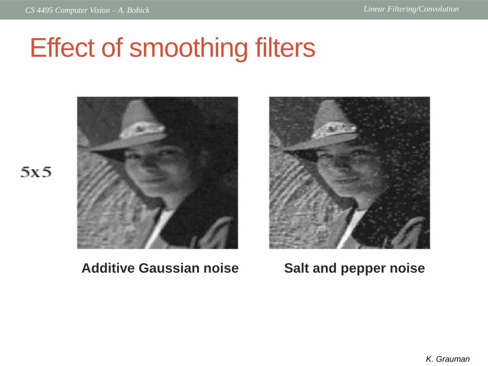
Effect of smoothing filters
Additive Gaussian noise Salt and pepper noise
K. Grauman
Linear Filtering/ConvolutionCS 4495 Computer Vision – A. Bobick
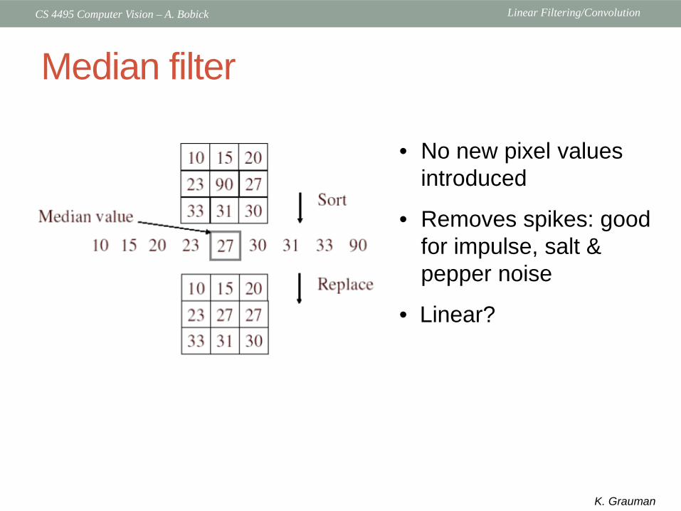
Median filter
• No new pixel values introduced
• Removes spikes: good for impulse, salt & pepper noise
• Linear?
K. Grauman
Linear Filtering/ConvolutionCS 4495 Computer Vision – A. Bobick
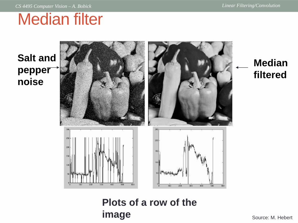
Median filter
Salt and pepper noise
Median filtered
Source: M. Hebert
Plots of a row of the image
Linear Filtering/ConvolutionCS 4495 Computer Vision – A. Bobick
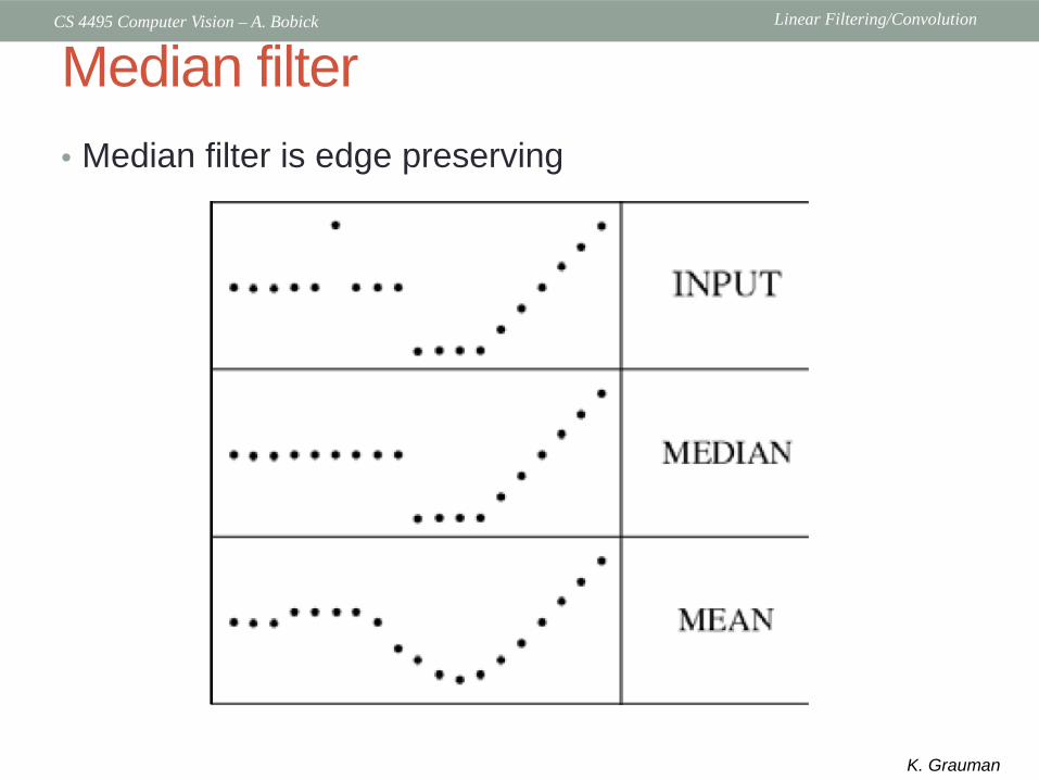
Median filter• Median filter is edge preserving
K. Grauman

Linear Filtering/ConvolutionCS 4495 Computer Vision – A. Bobick
To do:
• Problem set 0 available; due 11:59pm Thurs Aug 29th
• Problem set 1 – Filtering, Edges, Hough – will be handed out Aug 28th (Thurs) and is due Sun Sept 7, 11:59pm.