CS11.Supply Chain Management

eleven Supply Chain Management

CS11.1 Application Overview and Model Development CS11.2 Worksheets CS11.3 User Interface CS11.4 Procedures CS11.5 Re-solve Options CS11.6 Summary CS11.7 Extensions

case study OVERVIEW

CASE STUDY

CASE STUDY 11 Supply Chain Management 2

CS11.1 Application Overview and Model Development

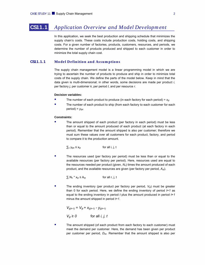
In this application, we seek the best production and shipping schedule that minimizes the supply chain’s costs. These costs include production costs, holding costs, and shipping costs. For a given number of factories, products, customers, resources, and periods, we determine the number of products produced and shipped to each customer in order to minimize the total supply chain cost.

CS11.1.1 Model Definition and Assumptions

The supply chain management model is a linear programming model in which we are trying to ascertain the number of products to produce and ship in order to minimize total costs of the supply chain. We define the parts of the model below. Keep in mind that the data given is multi-dimensional; in other words, some decisions are made per product i, per factory j, per customer k, per period t, and per resource r.

Decision variables: The number of each product to produce (in each factory for each period) = xijt The number of each product to ship (from each factory to each customer for each

period) = yijkt

Constraints: The amount shipped of each product (per factory in each period) must be less

than or equal to the amount produced of each product (at each factory in each period). Remember that the amount shipped is also per customer; therefore we must sum these values over all customers for each product, factory, and period to compare it to the production amount.

∑k yijkt ≤ xijt for all i, j, t

The resources used (per factory per period) must be less than or equal to the

available resources (per factory per period). Here, resources used are equal to the resources needed per product (given, Nri) times the amount produced of each product, and the available resources are given (per factory per period, Arjt).

∑i Nri * xijt ≤ Arjt for all r, j, t

The ending inventory (per product per factory per period, Vijt) must be greater

than 0 for each period. Here, we define the ending inventory of period t+1 as equal to the ending inventory in period t plus the amount produced in period t+1 minus the amount shipped in period t+1.

Vij(t+1) = Vijt + xij(t+1) - yij(t+1)

Vijt ≥ 0 for all i, j, t

The amount shipped (of each product from each factory to each customer) must

meet the demand per customer. Here, the demand has been given per product per customer per period, Dikt. Remember that the amount shipped is also per


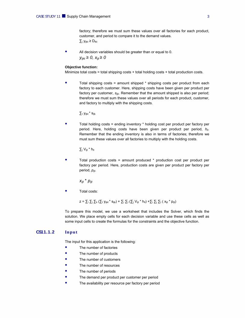
factory; therefore we must sum these values over all factories for each product, customer, and period to compare it to the demand values. ∑j yijkt ≥ Dikt

All decision variables should be greater than or equal to 0.

yijkt ≥ 0, xijt ≥ 0

Objective function: Minimize total costs = total shipping costs + total holding costs + total production costs.

Total shipping costs = amount shipped * shipping costs per product from each

factory to each customer. Here, shipping costs have been given per product per factory per customer, sijk. Remember that the amount shipped is also per period; therefore we must sum these values over all periods for each product, customer, and factory to multiply with the shipping costs.

∑t yijkt * sijk

Total holding costs = ending inventory * holding cost per product per factory per

period. Here, holding costs have been given per product per period, hit. Remember that the ending inventory is also in terms of factories; therefore we must sum these values over all factories to multiply with the holding costs.

∑j Vijt * hit

Total production costs = amount produced * production cost per product per

factory per period. Here, production costs are given per product per factory per period, pijt.

xijt * pijt

Total costs:

z = ∑i ∑j ∑k (∑t yijkt * sijk) + ∑i ∑t (∑j Vijt * hit) +∑i ∑j ∑t ( xijt * pijt)

To prepare this model, we use a worksheet that includes the Solver, which finds the solution. We place empty cells for each decision variable and use these cells as well as some input cells to create the formulas for the constraints and the objective function.

CS11.1.2 Input

The input for this application is the following: The number of factories The number of products The number of customers The number of resources The number of periods The demand per product per customer per period The availability per resource per factory per period


The need per resource per product The holding costs per product per period The production costs per product per factory per period The shipping costs per product per factory per customer The initial inventory per product per factory

CS11.1.3 Output

The output for this application is the following: The total supply chain costs The production plan per product per factory per period The shipping plan per product per factory per customer per period The total shipping costs per product per factory per customer The total holding costs per product per factory per period The total production costs per product per factory per period

CS11.2 Worksheets

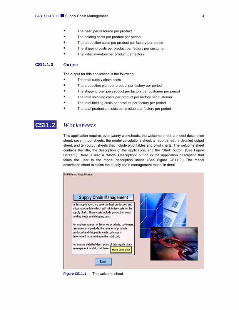
This application requires over twenty worksheets: the welcome sheet, a model description sheet, seven input sheets, the model calculations sheet, a report sheet, a detailed output sheet, and ten output sheets that include pivot tables and pivot charts. The welcome sheet contains the title, the description of the application, and the “Start” button. (See Figure CS11.1.) There is also a “Model Description” button in the application description that takes the user to the model description sheet. (See Figure CS11.2.) The model description sheet explains the supply chain management model in detail.

Figure CS11.1 The welcome sheet.


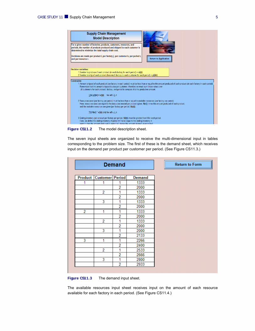
Figure CS11.2 The model description sheet.

The seven input sheets are organized to receive the multi-dimensional input in tables corresponding to the problem size. The first of these is the demand sheet, which receives input on the demand per product per customer per period. (See Figure CS11.3.)

Figure CS11.3 The demand input sheet.

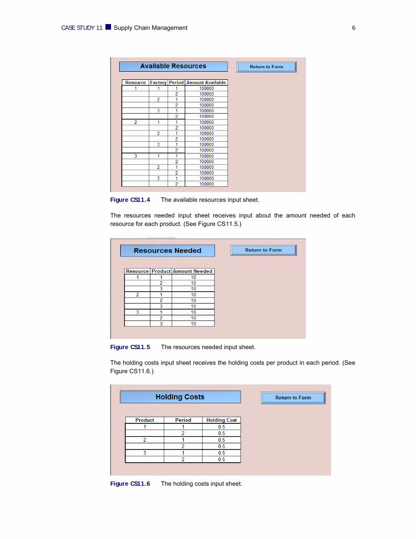
The available resources input sheet receives input on the amount of each resource available for each factory in each period. (See Figure CS11.4.)


Figure CS11.4 The available resources input sheet.

The resources needed input sheet receives input about the amount needed of each resource for each product. (See Figure CS11.5.)

Figure CS11.5 The resources needed input sheet.

The holding costs input sheet receives the holding costs per product in each period. (See Figure CS11.6.)

Figure CS11.6 The holding costs input sheet.


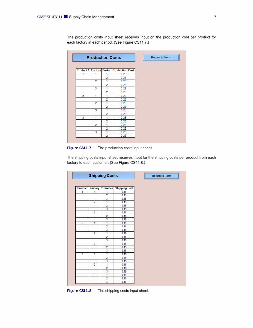
The production costs input sheet receives input on the production cost per product for each factory in each period. (See Figure CS11.7.)

Figure CS11.7 The production costs input sheet.

The shipping costs input sheet receives input for the shipping costs per product from each factory to each customer. (See Figure CS11.8.)

Figure CS11.8 The shipping costs input sheet.


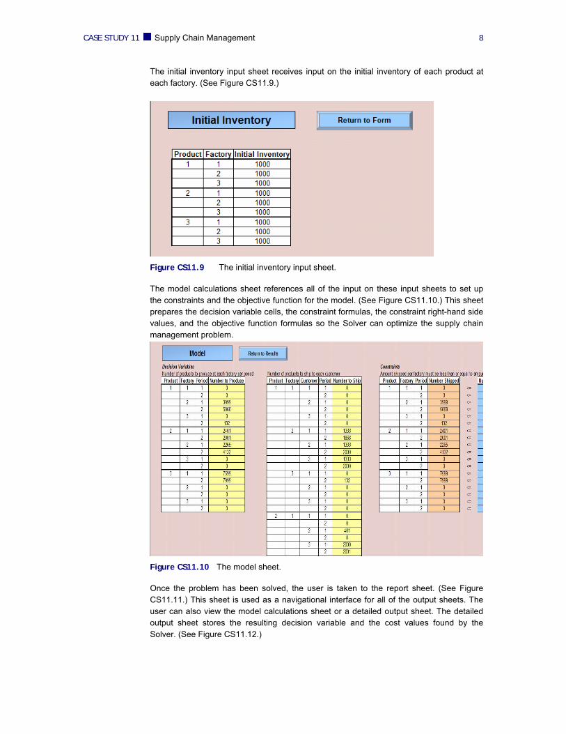
The initial inventory input sheet receives input on the initial inventory of each product at each factory. (See Figure CS11.9.)

Figure CS11.9 The initial inventory input sheet.

The model calculations sheet references all of the input on these input sheets to set up the constraints and the objective function for the model. (See Figure CS11.10.) This sheet prepares the decision variable cells, the constraint formulas, the constraint right-hand side values, and the objective function formulas so the Solver can optimize the supply chain management problem.

Figure CS11.10 The model sheet.

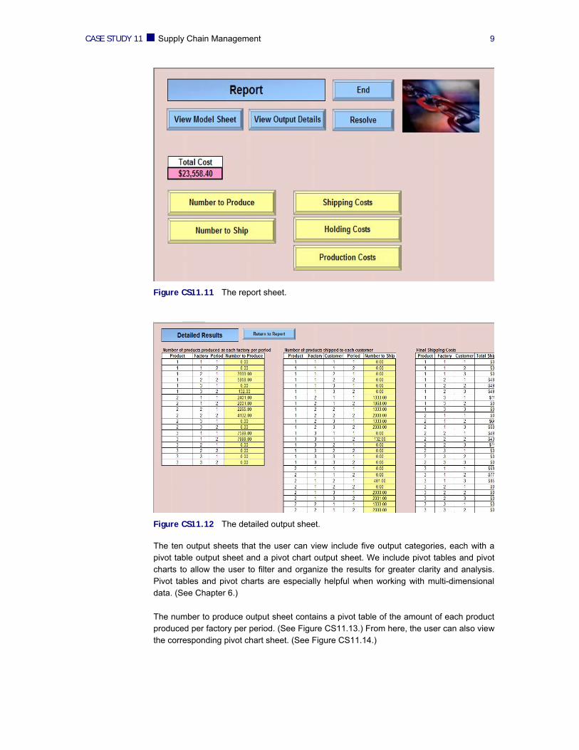
Once the problem has been solved, the user is taken to the report sheet. (See Figure CS11.11.) This sheet is used as a navigational interface for all of the output sheets. The user can also view the model calculations sheet or a detailed output sheet. The detailed output sheet stores the resulting decision variable and the cost values found by the Solver. (See Figure CS11.12.)


Figure CS11.11 The report sheet.

Figure CS11.12 The detailed output sheet.

The ten output sheets that the user can view include five output categories, each with a pivot table output sheet and a pivot chart output sheet. We include pivot tables and pivot charts to allow the user to filter and organize the results for greater clarity and analysis. Pivot tables and pivot charts are especially helpful when working with multi-dimensional data. (See Chapter 6.)

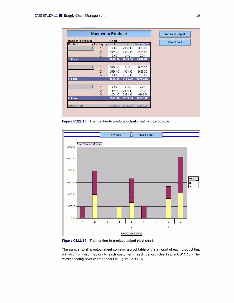
The number to produce output sheet contains a pivot table of the amount of each product produced per factory per period. (See Figure CS11.13.) From here, the user can also view the corresponding pivot chart sheet. (See Figure CS11.14.)


Figure CS11.13 The number to produce output sheet with pivot table.

Figure CS11.14 The number to produce output pivot chart.

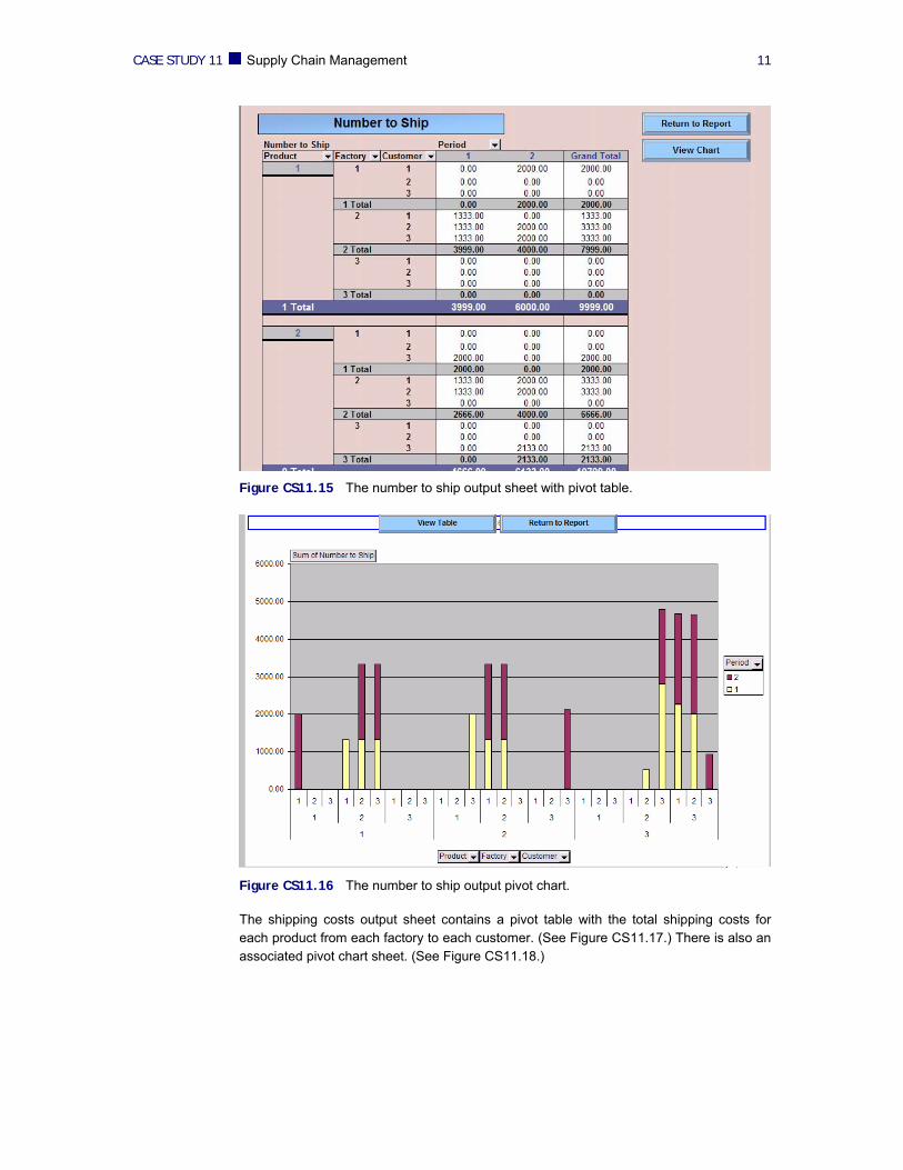
The number to ship output sheet contains a pivot table of the amount of each product that will ship from each factory to each customer in each period. (See Figure CS11.15.) The corresponding pivot chart appears in Figure CS11.16.


Figure CS11.15 The number to ship output sheet with pivot table.

Figure CS11.16 The number to ship output pivot chart.

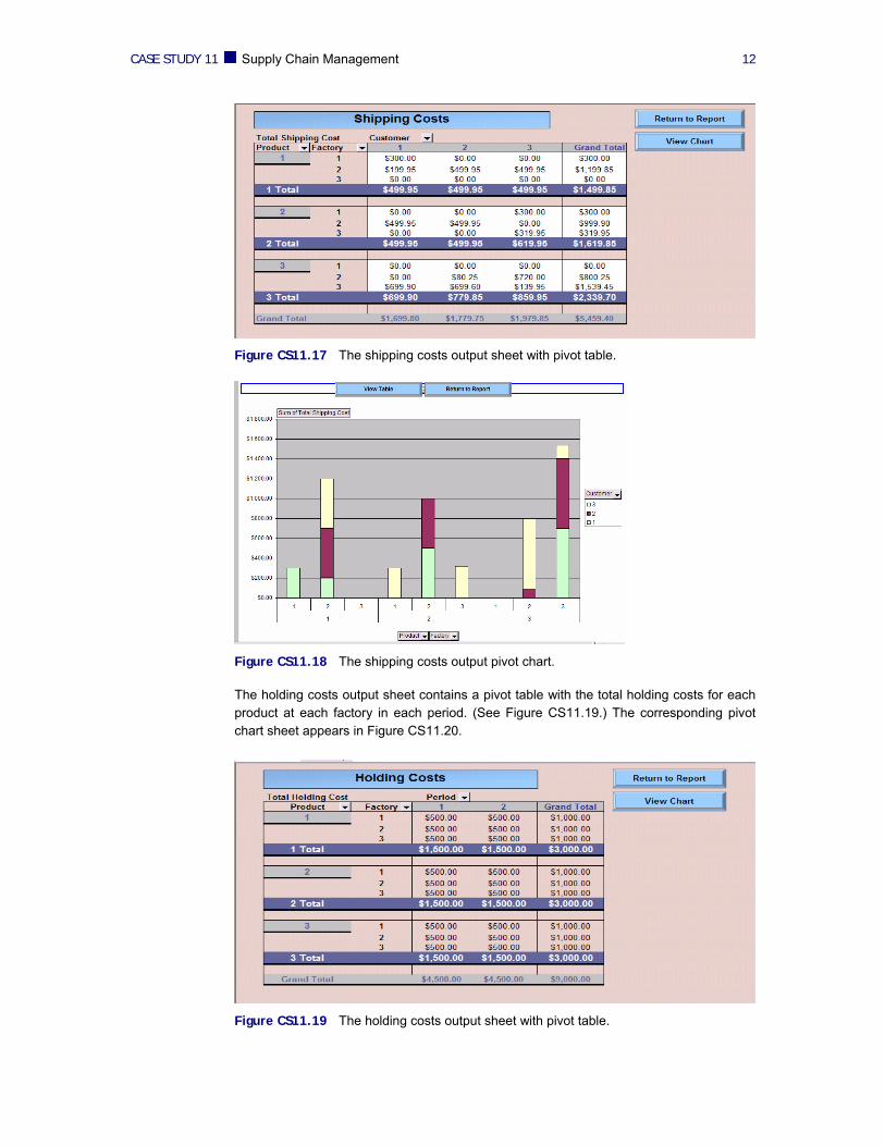
The shipping costs output sheet contains a pivot table with the total shipping costs for each product from each factory to each customer. (See Figure CS11.17.) There is also an associated pivot chart sheet. (See Figure CS11.18.)


Figure CS11.17 The shipping costs output sheet with pivot table.

Figure CS11.18 The shipping costs output pivot chart.

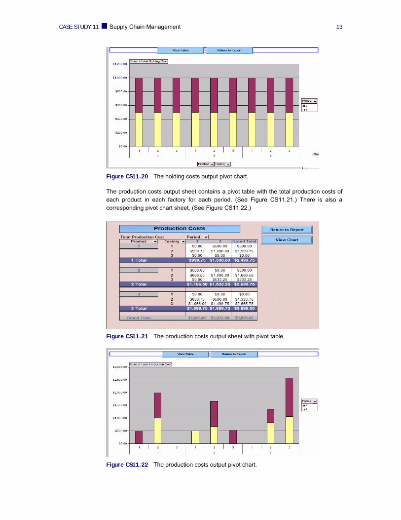
The holding costs output sheet contains a pivot table with the total holding costs for each product at each factory in each period. (See Figure CS11.19.) The corresponding pivot chart sheet appears in Figure CS11.20.

Figure CS11.19 The holding costs output sheet with pivot table.


Figure CS11.20 The holding costs output pivot chart.

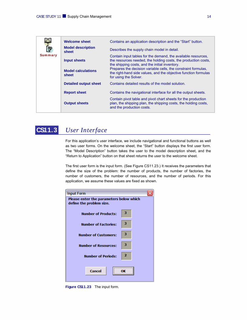
The production costs output sheet contains a pivot table with the total production costs of each product in each factory for each period. (See Figure CS11.21.) There is also a corresponding pivot chart sheet. (See Figure CS11.22.)

Figure CS11.21 The production costs output sheet with pivot table.

Figure CS11.22 The production costs output pivot chart.


CS11.3 User Interface

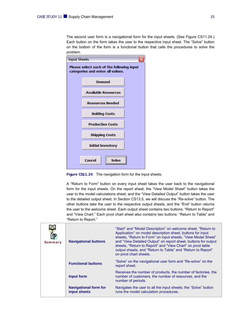
For this application’s user interface, we include navigational and functional buttons as well as two user forms. On the welcome sheet, the “Start” button displays the first user form. The “Model Description” button takes the user to the model description sheet, and the “Return to Application” button on that sheet returns the user to the welcome sheet. The first user form is the input form. (See Figure CS11.23.) It receives the parameters that define the size of the problem: the number of products, the number of factories, the number of customers, the number of resources, and the number of periods. For this application, we assume these values are fixed as shown.

Figure CS11.23 The input form.

Welcome sheet Contains an application description and the “Start” button. Model description sheet Describes the supply chain model in detail.

Input sheets Contain input tables for the demand, the available resources, the resources needed, the holding costs, the production costs, the shipping costs, and the initial inventory.

Model calculations sheet

Prepares the decision variable cells, the constraint formulas, the right-hand side values, and the objective function formulas for using the Solver.

Detailed output sheet Contains detailed results of the model solution.

Report sheet Contains the navigational interface for all the output sheets.

Output sheets Contain pivot table and pivot chart sheets for the production plan, the shipping plan, the shipping costs, the holding costs, and the production costs.

Summary


The second user form is a navigational form for the input sheets. (See Figure CS11.24.) Each button on the form takes the user to the respective input sheet. The “Solve” button on the bottom of the form is a functional button that calls the procedures to solve the problem.

Figure CS11.24 The navigation form for the input sheets.

A “Return to Form” button on every input sheet takes the user back to the navigational form for the input sheets. On the report sheet, the “View Model Sheet” button takes the user to the model calculations sheet, and the “View Detailed Output” button takes the user to the detailed output sheet. In Section CS13.5, we will discuss the “Re-solve” button. The other buttons take the user to the respective output sheets, and the “End” button returns the user to the welcome sheet. Each output sheet contains two buttons: “Return to Report” and “View Chart.” Each pivot chart sheet also contains two buttons: “Return to Table” and “Return to Report.”

Navigational buttons

“Start” and “Model Description” on welcome sheet, “Return to Application” on model description sheet, buttons for input sheets, “Return to Form” on input sheets, “View Model Sheet” and “View Detailed Output” on report sheet, buttons for output sheets, “Return to Report” and “View Chart” on pivot table output sheets, and “Return to Table” and “Return to Report” on pivot chart sheets.

Functional buttons “Solve” on the navigational user form and “Re-solve” on the report sheet.

Input form Receives the number of products, the number of factories, the number of customers, the number of resources, and the number of periods.

Navigational form for input sheets

Navigates the user to all the input sheets; the “Solve” button runs the model calculation procedures.

Summary


CS11.4 Procedures

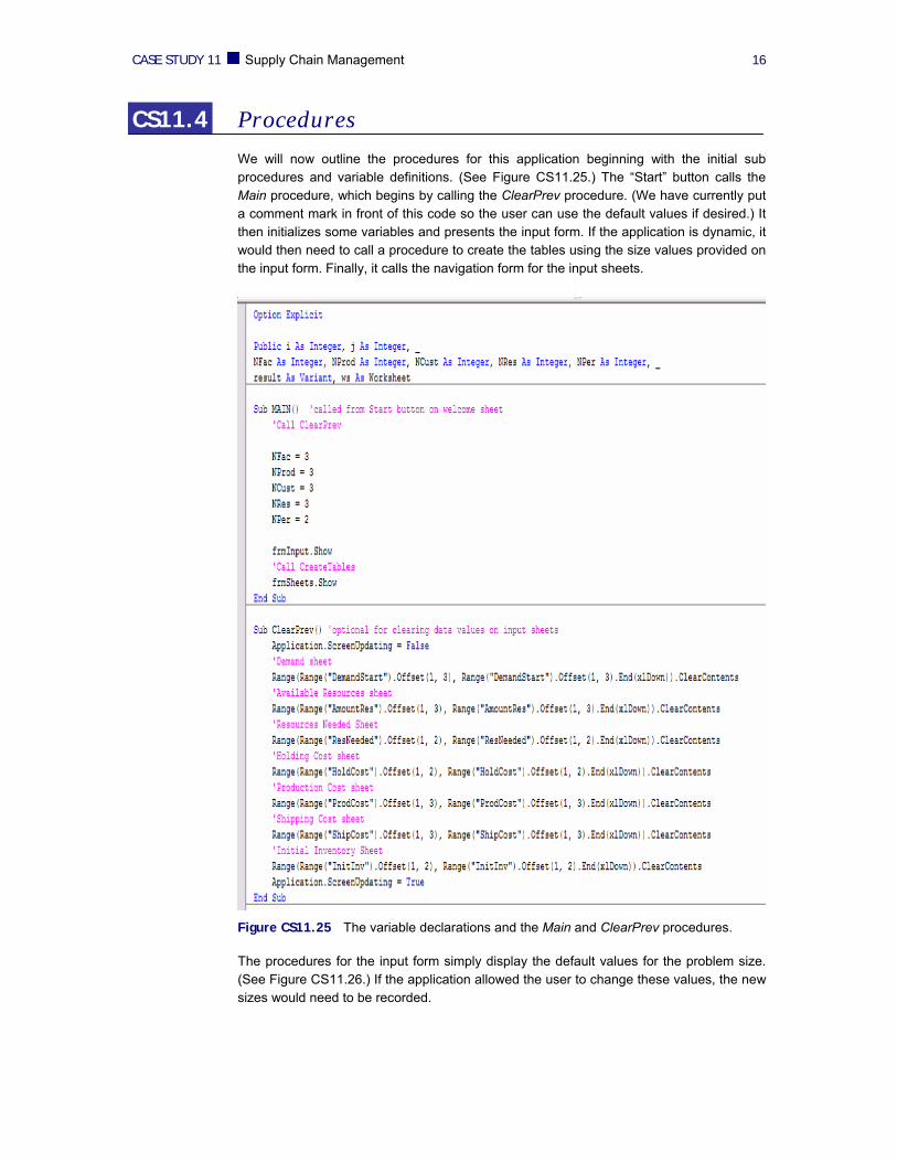
We will now outline the procedures for this application beginning with the initial sub procedures and variable definitions. (See Figure CS11.25.) The “Start” button calls the Main procedure, which begins by calling the ClearPrev procedure. (We have currently put a comment mark in front of this code so the user can use the default values if desired.) It then initializes some variables and presents the input form. If the application is dynamic, it would then need to call a procedure to create the tables using the size values provided on the input form. Finally, it calls the navigation form for the input sheets.

Figure CS11.25 The variable declarations and the Main and ClearPrev procedures.

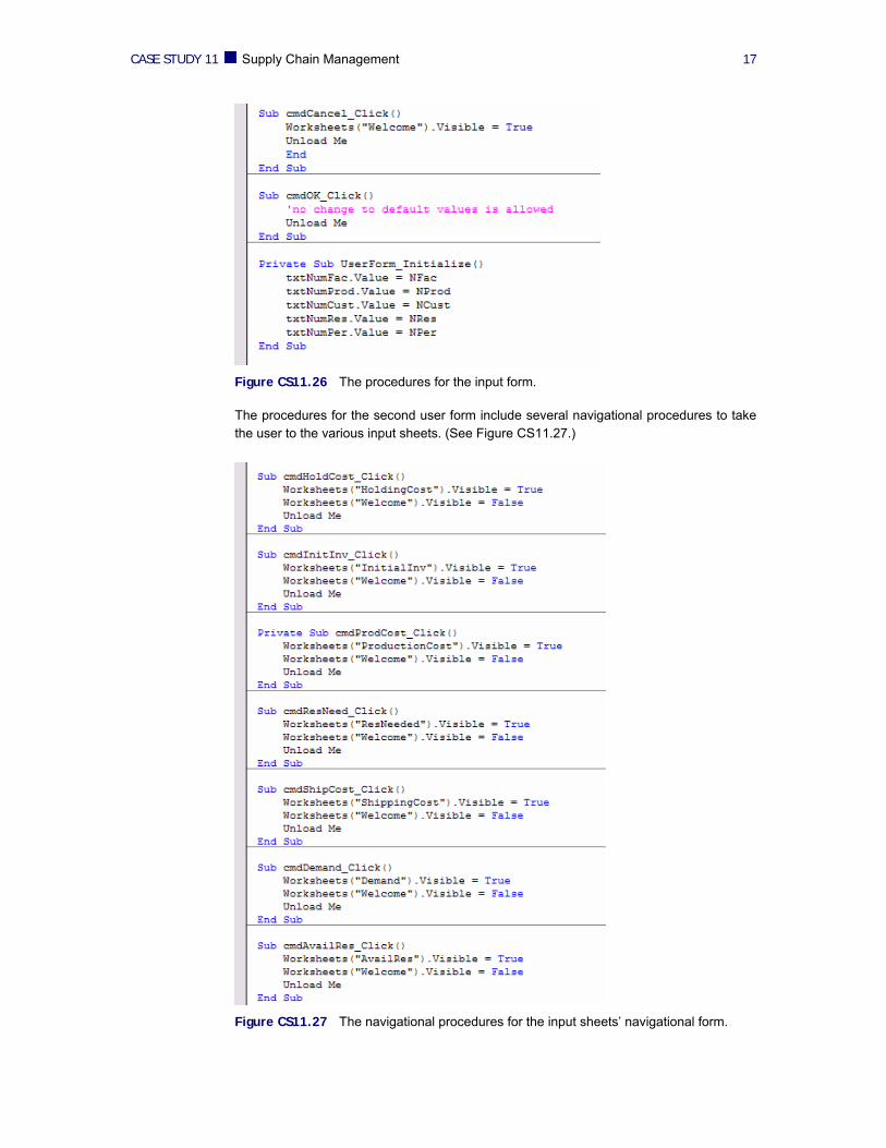
The procedures for the input form simply display the default values for the problem size. (See Figure CS11.26.) If the application allowed the user to change these values, the new sizes would need to be recorded.


Figure CS11.26 The procedures for the input form.

The procedures for the second user form include several navigational procedures to take the user to the various input sheets. (See Figure CS11.27.)

Figure CS11.27 The navigational procedures for the input sheets’ navigational form.


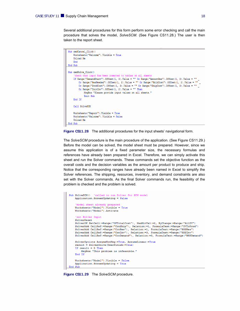
Several additional procedures for this form perform some error checking and call the main procedure that solves the model, SolveSCM. (See Figure CS11.28.) The user is then taken to the report sheet.

Figure CS11.28 The additional procedures for the input sheets’ navigational form.

The SolveSCM procedure is the main procedure of the application. (See Figure CS11.29.) Before the model can be solved, the model sheet must be prepared. However, since we assume this application is of a fixed parameter size, the necessary formulas and references have already been prepared in Excel. Therefore, we can simply activate this sheet and run the Solver commands. These commands set the objective function as the overall costs and the decision variables as the amount per product to produce and ship. Notice that the corresponding ranges have already been named in Excel to simplify the Solver references. The shipping, resources, inventory, and demand constraints are also set with the Solver commands. As the final Solver commands run, the feasibility of the problem is checked and the problem is solved.

Figure CS11.29 The SolveSCM procedure.


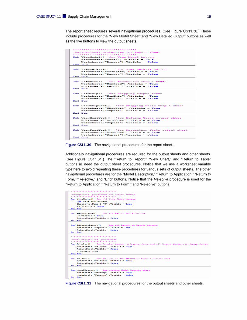
The report sheet requires several navigational procedures. (See Figure CS11.30.) These include procedures for the “View Model Sheet” and “View Detailed Output” buttons as well as the five buttons to view the output sheets.

Figure CS11.30 The navigational procedures for the report sheet.

Additionally navigational procedures are required for the output sheets and other sheets. (See Figure CS11.31.) The “Return to Report,” “View Chart,” and “Return to Table” buttons all need the output sheet procedures. Notice that we use a worksheet variable type here to avoid repeating these procedures for various sets of output sheets. The other navigational procedures are for the “Model Description,” “Return to Application,” “Return to Form,” “Re-solve,” and “End” buttons. Notice that the Re-solve procedure is used for the “Return to Application,” “Return to Form,” and “Re-solve” buttons.

Figure CS11.31 The navigational procedures for the output sheets and other sheets.


CS11.5 Re-solve Options

The user can re-solve this application by pressing the “Re-solve” button on the report sheet. This button is assigned to the Re-solve procedure, which brings the user back to the welcome sheet and re-displays the navigational form for the input sheets. (See Figure CS11.31.) This procedure allows the user to change the input values and re-solve the model calculations. He or she can then return to the report sheet to view all of the output.

CS11.6 Summary

In this application, we seek the best production and shipping schedule that minimizes the supply chain’s costs. These costs include the production costs, the holding costs, and the shipping costs.

This application requires over twenty worksheets: the welcome sheet, a model description sheet, seven input sheets, the model calculations sheet, a report sheet, a detailed output sheet, and ten output sheets that include pivot tables and pivot charts.

For this application’s interface, we use navigational and functional buttons as well as two user forms.

Several procedures in this application initialize and perform the model calculations to find the optimal production and shipping plans that minimize overall costs.

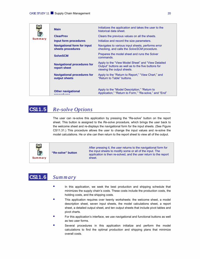
Main Initializes the application and takes the user to the historical data sheet.

ClearPrev Clears the previous values on all the sheets. Input form procedures Initialize and record the size parameters. Navigational form for input sheets procedures

Navigates to various input sheets, performs error checking, and calls the SolveSCM procedure.

SolveSCM Prepares the model sheet and runs the Solver commands.

Navigational procedures for report sheet

Apply to the “View Model Sheet” and “View Detailed Output” buttons as well as to the five buttons for viewing the output sheets.

Navigational procedures for output sheets

Apply to the “Return to Report,” “View Chart,” and “Return to Table” buttons.

Other navigational procedures

Apply to the “Model Description,” “Return to Application,” “Return to Form,” “Re-solve,” and “End”

Summary

“Re-solve” button After pressing it, the user returns to the navigational form for the input sheets to modify some or all of the input. The application is then re-solved, and the user return to the report sheet.

Summary


The user can re-solve the application by pressing the “Re-solve” button on the report sheet; he or she revisits the input sheets, modifies the values, and re-solves the model.

CS11.7 Extensions

If the user were able to change the size parameters of the problem, which sheets would this affect?

If the user were able to change the size parameters of the problem, which procedures would this affect?

If the user were able to change the size parameters of the problem, what are some new procedures that would need to be created? Make these changes to the application so it is dynamic. What other re-solve options are now possible?

Documents

CS11.Supply Chain Management