CS252/Kubiatowicz Lec 21.1 11/10/99 CS252 Graduate Computer Architecture Lecture 21 I/O Introduction Prof. John Kubiatowicz Computer Science 252 Fall 1998

CS252/KubiatowiczLec 21.1

11/10/99

CS252Graduate Computer Architecture

Lecture 21

I/O Introduction

Prof. John Kubiatowicz

Computer Science 252

Fall 1998


11/10/99

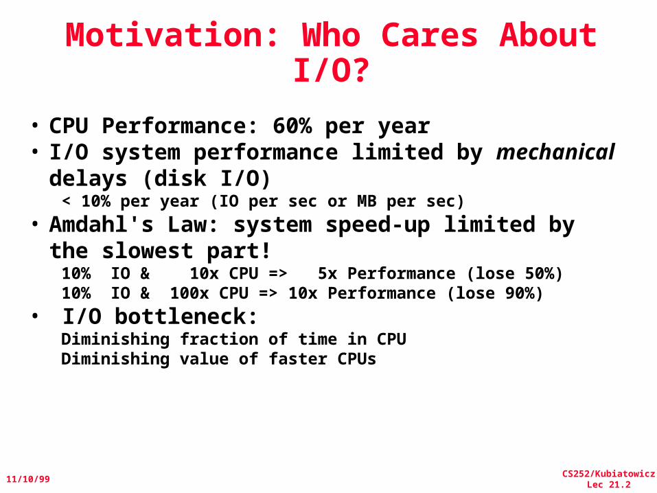
Motivation: Who Cares About I/O?

• CPU Performance: 60% per year• I/O system performance limited by mechanical

delays (disk I/O)< 10% per year (IO per sec or MB per sec)

• Amdahl's Law: system speed-up limited by the slowest part!

10% IO & 10x CPU => 5x Performance (lose 50%)10% IO & 100x CPU => 10x Performance (lose 90%)

• I/O bottleneck: Diminishing fraction of time in CPUDiminishing value of faster CPUs


11/10/99

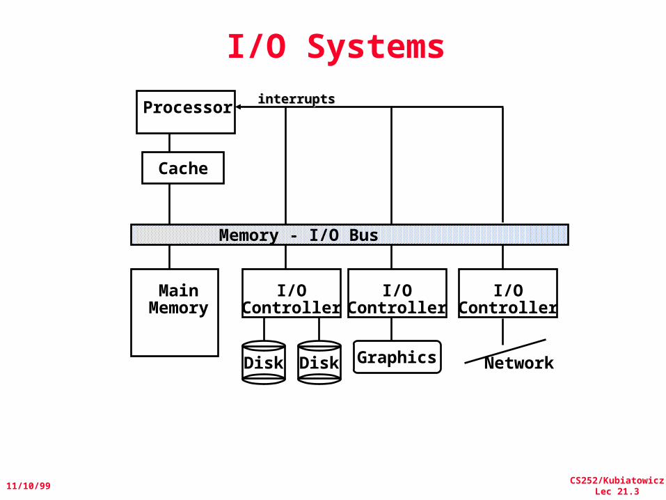
I/O Systems

Processor

Cache

Memory - I/O Bus

MainMemory

I/OController

Disk Disk

I/OController

I/OController

Graphics Network

interruptsinterrupts


11/10/99

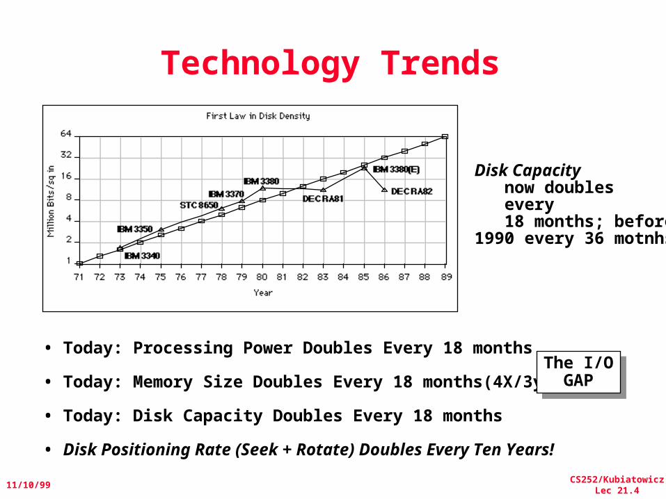
Technology Trends

Disk Capacity now doubles every 18 months; before1990 every 36 motnhs

• Today: Processing Power Doubles Every 18 months

• Today: Memory Size Doubles Every 18 months(4X/3yr)

• Today: Disk Capacity Doubles Every 18 months

• Disk Positioning Rate (Seek + Rotate) Doubles Every Ten Years!

The I/OGAP

The I/OGAP


11/10/99

Storage Technology Drivers

• Driven by the prevailing computing paradigm– 1950s: migration from batch to on-line processing– 1990s: migration to ubiquitous computing

» computers in phones, books, cars, video cameras, …

» nationwide fiber optical network with wireless tails

• Effects on storage industry:– Embedded storage

» smaller, cheaper, more reliable, lower power– Data utilities

» high capacity, hierarchically managed storage


11/10/99

Historical Perspective• 1956 IBM Ramac — early 1970s Winchester

– Developed for mainframe computers, proprietary interfaces– Steady shrink in form factor: 27 in. to 14 in.

• 1970s developments– 5.25 inch floppy disk formfactor (microcode into mainframe)– early emergence of industry standard disk interfaces

» ST506, SASI, SMD, ESDI

• Early 1980s– PCs and first generation workstations

• Mid 1980s– Client/server computing – Centralized storage on file server

» accelerates disk downsizing: 8 inch to 5.25 inch– Mass market disk drives become a reality

» industry standards: SCSI, IPI, IDE» 5.25 inch drives for standalone PCs, End of proprietary interfaces


11/10/99

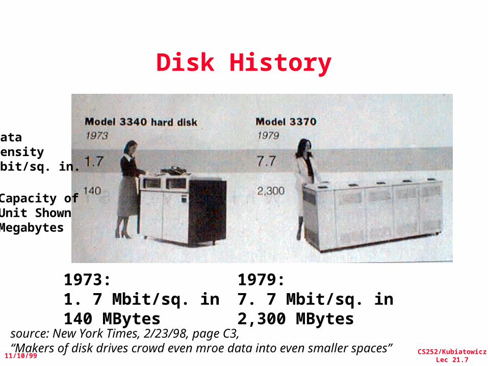
Disk History

Data densityMbit/sq. in.

Capacity ofUnit ShownMegabytes

1973:1. 7 Mbit/sq. in140 MBytes

1979:7. 7 Mbit/sq. in2,300 MBytes

source: New York Times, 2/23/98, page C3, “Makers of disk drives crowd even mroe data into even smaller spaces”


11/10/99

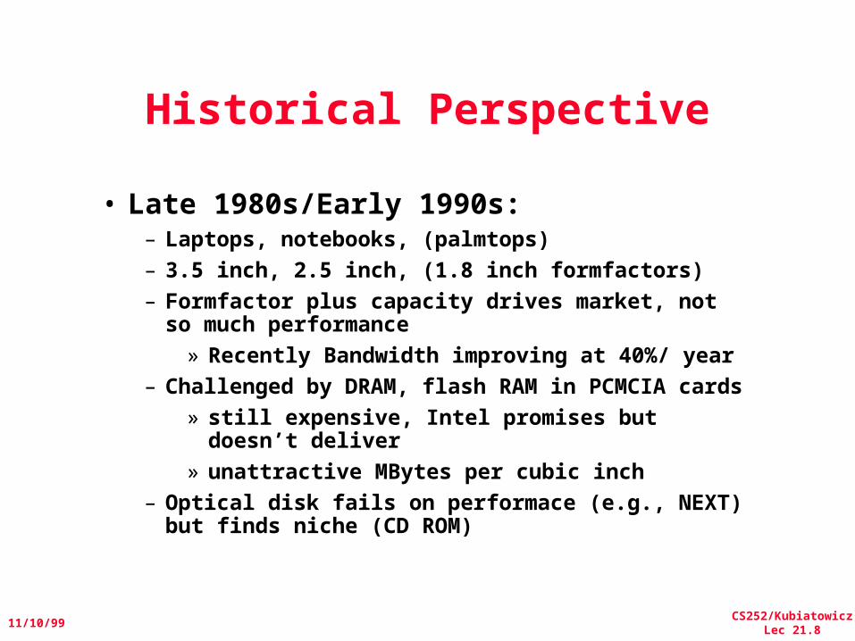
Historical Perspective

• Late 1980s/Early 1990s:– Laptops, notebooks, (palmtops)– 3.5 inch, 2.5 inch, (1.8 inch formfactors)– Formfactor plus capacity drives market, not so

much performance» Recently Bandwidth improving at 40%/ year

– Challenged by DRAM, flash RAM in PCMCIA cards» still expensive, Intel promises but doesn’t

deliver» unattractive MBytes per cubic inch

– Optical disk fails on performace (e.g., NEXT) but finds niche (CD ROM)


11/10/99

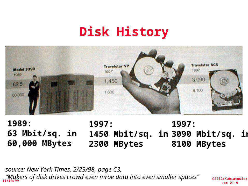
Disk History

1989:63 Mbit/sq. in60,000 MBytes

1997:1450 Mbit/sq. in2300 MBytes


1997:3090 Mbit/sq. in8100 MBytes


11/10/99

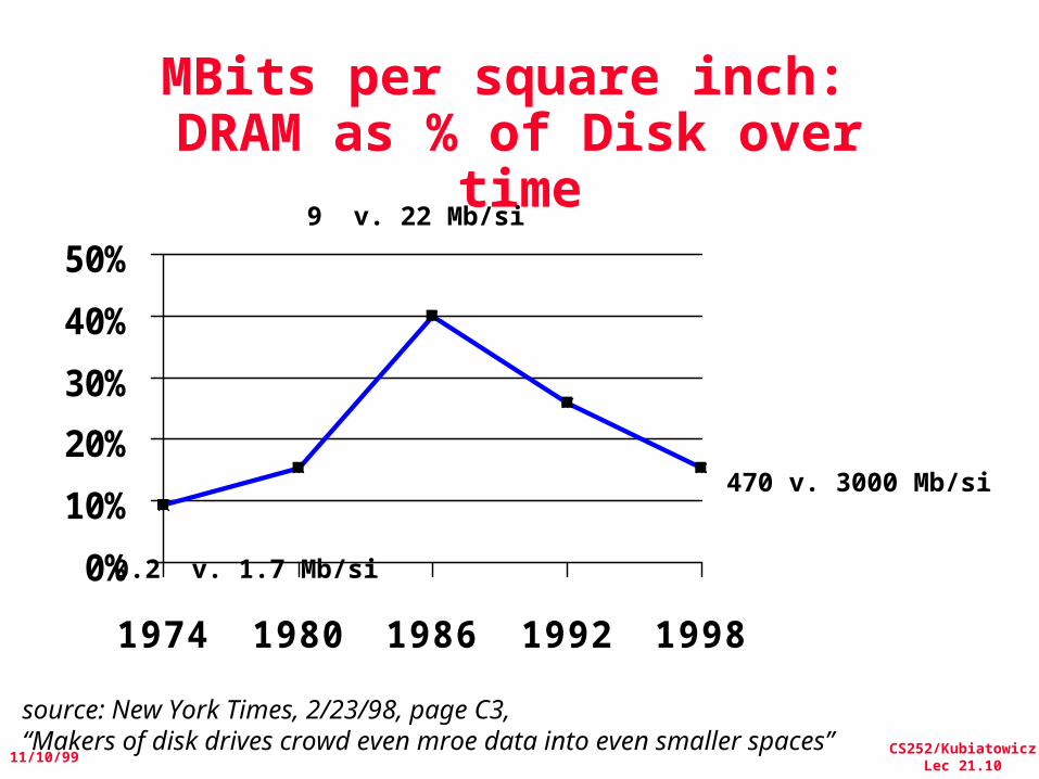
MBits per square inch: DRAM as % of Disk over

time

0%

10%

20%

30%

40%

50%

1974 1980 1986 1992 1998


470 v. 3000 Mb/si

9 v. 22 Mb/si

0.2 v. 1.7 Mb/si


11/10/99

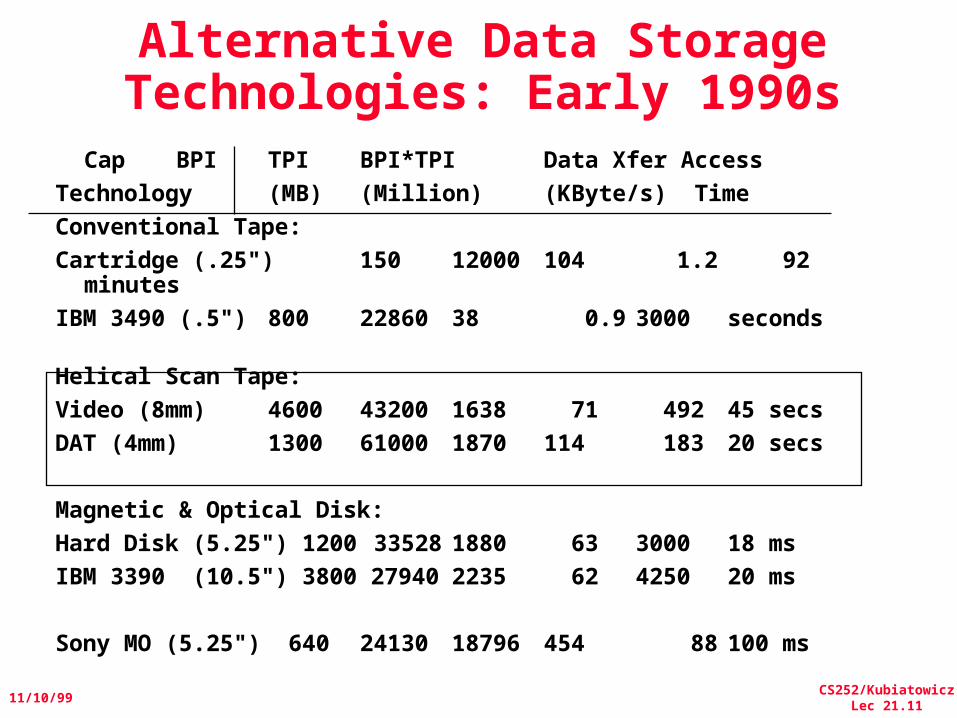
Alternative Data Storage Technologies: Early 1990s

Cap BPI TPI BPI*TPI Data Xfer Access

Technology (MB) (Million) (KByte/s) Time

Conventional Tape:

Cartridge (.25") 150 12000 104 1.2 92 minutes

IBM 3490 (.5") 800 22860 38 0.9 3000 seconds

Helical Scan Tape:

Video (8mm) 4600 43200 1638 71 492 45 secs

DAT (4mm) 1300 61000 1870 114 183 20 secs

Magnetic & Optical Disk:

Hard Disk (5.25") 1200 33528 1880 63 3000 18 ms

IBM 3390 (10.5") 3800 27940 2235 62 4250 20 ms

Sony MO (5.25") 640 24130 18796 454 88 100 ms


11/10/99

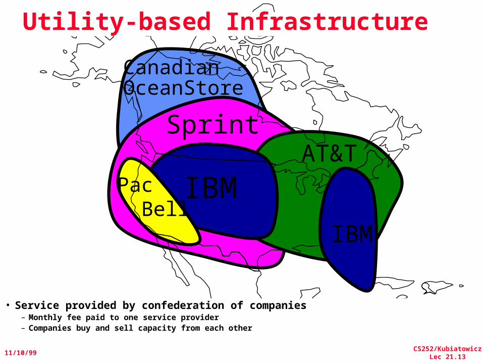
Option 2:The Oceanic Data Utility:

Global-Scale Persistent Storage


11/10/99

Pac Bell

Sprint

IBMAT&T

CanadianOceanStore

• Service provided by confederation of companies– Monthly fee paid to one service provider– Companies buy and sell capacity from each other

IBM

Utility-based Infrastructure


11/10/99

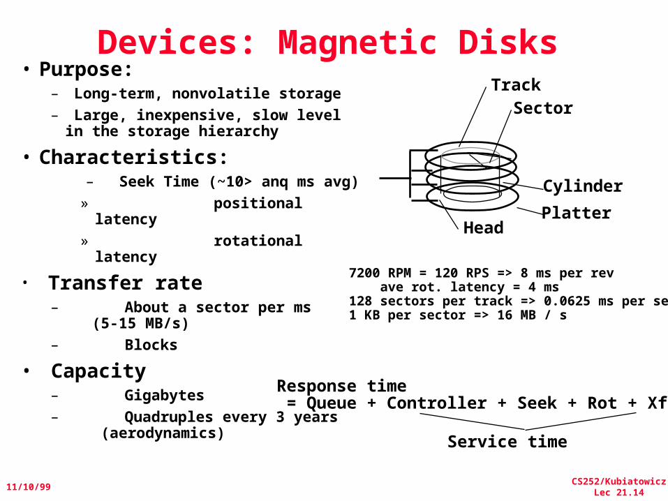
Devices: Magnetic Disks

SectorTrack

Cylinder

HeadPlatter

• Purpose:– Long-term, nonvolatile storage– Large, inexpensive, slow level in

the storage hierarchy

• Characteristics:– Seek Time (~10> anq ms avg)» positional

latency» rotational

latency

• Transfer rate– About a sector per ms

(5-15 MB/s)– Blocks

• Capacity– Gigabytes– Quadruples every 3 years

(aerodynamics)

7200 RPM = 120 RPS => 8 ms per rev ave rot. latency = 4 ms128 sectors per track => 0.0625 ms per sector1 KB per sector => 16 MB / s

Response time = Queue + Controller + Seek + Rot + Xfer

Service time


11/10/99

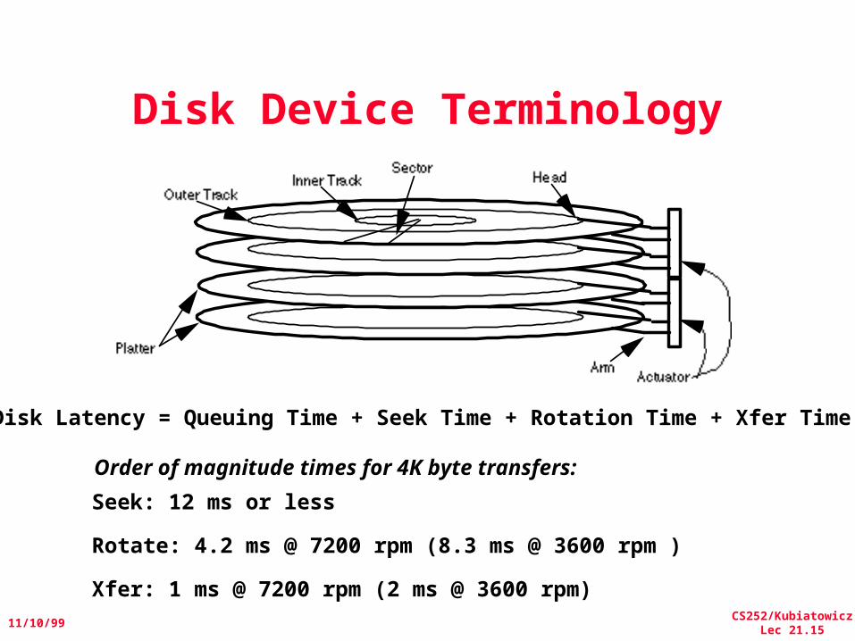
Disk Device Terminology

Disk Latency = Queuing Time + Seek Time + Rotation Time + Xfer Time

Order of magnitude times for 4K byte transfers:

Seek: 12 ms or less

Rotate: 4.2 ms @ 7200 rpm (8.3 ms @ 3600 rpm )

Xfer: 1 ms @ 7200 rpm (2 ms @ 3600 rpm)


11/10/99

Nano-layered Disk Heads• Special sensitivity of Disk head comes from “Giant

Magneto-Resistive effect” or (GMR) • IBM is leader in this technology

– Same technology as TMJ-RAM breakthrough we described in earlier class.

Coil for writing


11/10/99

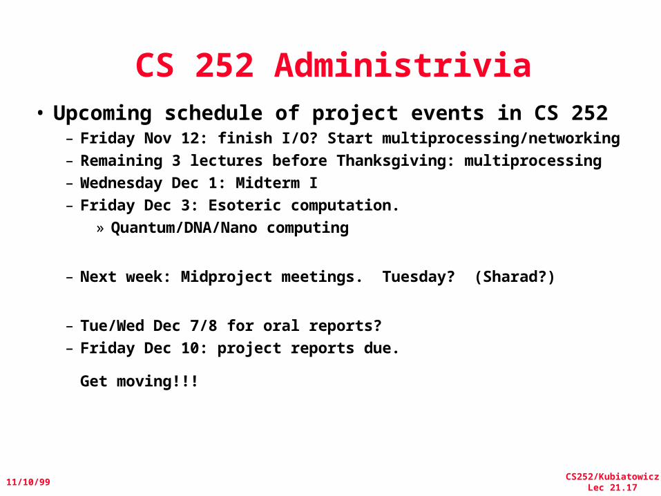
CS 252 Administrivia• Upcoming schedule of project events in CS 252

– Friday Nov 12: finish I/O? Start multiprocessing/networking– Remaining 3 lectures before Thanksgiving: multiprocessing– Wednesday Dec 1: Midterm I – Friday Dec 3: Esoteric computation.

» Quantum/DNA/Nano computing

– Next week: Midproject meetings. Tuesday? (Sharad?)

– Tue/Wed Dec 7/8 for oral reports?– Friday Dec 10: project reports due.

Get moving!!!


11/10/99

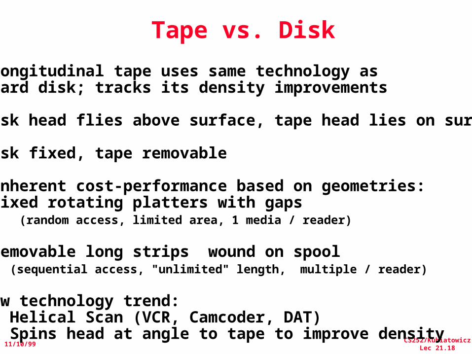
Tape vs. Disk

• Longitudinal tape uses same technology as hard disk; tracks its density improvements

• Disk head flies above surface, tape head lies on surface

• Disk fixed, tape removable

• Inherent cost-performance based on geometries: fixed rotating platters with gaps (random access, limited area, 1 media / reader)vs. removable long strips wound on spool (sequential access, "unlimited" length, multiple / reader)

• New technology trend: Helical Scan (VCR, Camcoder, DAT) Spins head at angle to tape to improve density


11/10/99

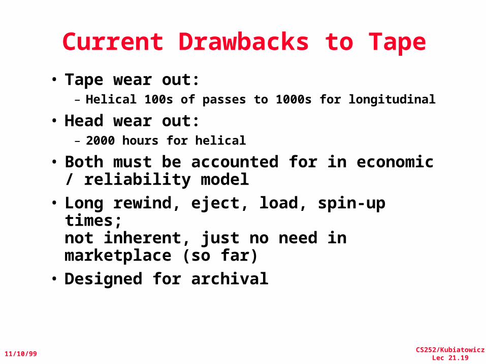
Current Drawbacks to Tape• Tape wear out:

– Helical 100s of passes to 1000s for longitudinal

• Head wear out: – 2000 hours for helical

• Both must be accounted for in economic / reliability model

• Long rewind, eject, load, spin-up times; not inherent, just no need in marketplace (so far)

• Designed for archival


11/10/99

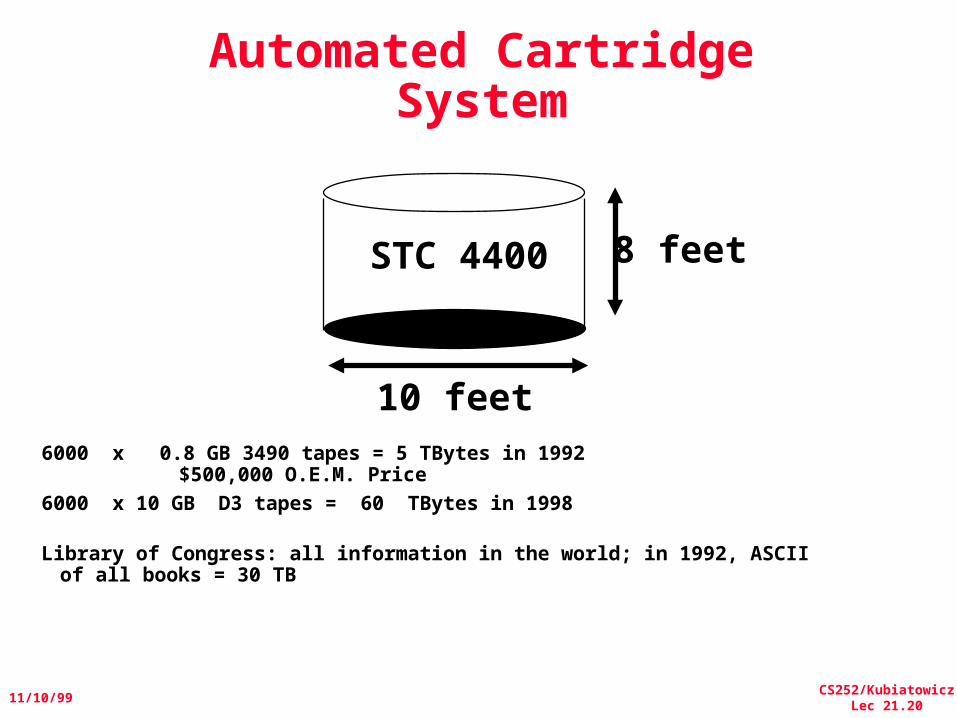
Automated Cartridge System

STC 4400

6000 x 0.8 GB 3490 tapes = 5 TBytes in 1992 $500,000 O.E.M. Price

6000 x 10 GB D3 tapes = 60 TBytes in 1998

Library of Congress: all information in the world; in 1992, ASCII of all books = 30 TB

8 feet

10 feet


11/10/99

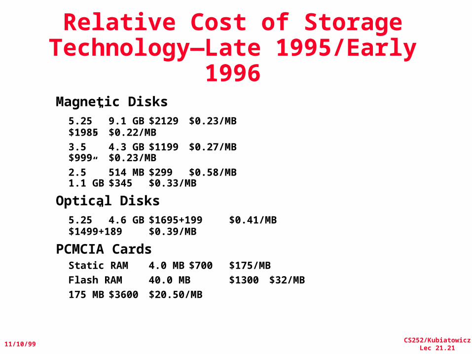
Relative Cost of Storage Technology—Late 1995/Early

1996Magnetic Disks

5.25” 9.1 GB $2129 $0.23/MB$1985 $0.22/MB

3.5” 4.3 GB $1199 $0.27/MB$999 $0.23/MB

2.5” 514 MB $299 $0.58/MB1.1 GB $345 $0.33/MB

Optical Disks5.25” 4.6 GB $1695+199 $0.41/MB

$1499+189 $0.39/MB

PCMCIA CardsStatic RAM 4.0 MB $700 $175/MBFlash RAM 40.0 MB $1300 $32/MB

175 MB $3600 $20.50/MB


11/10/99

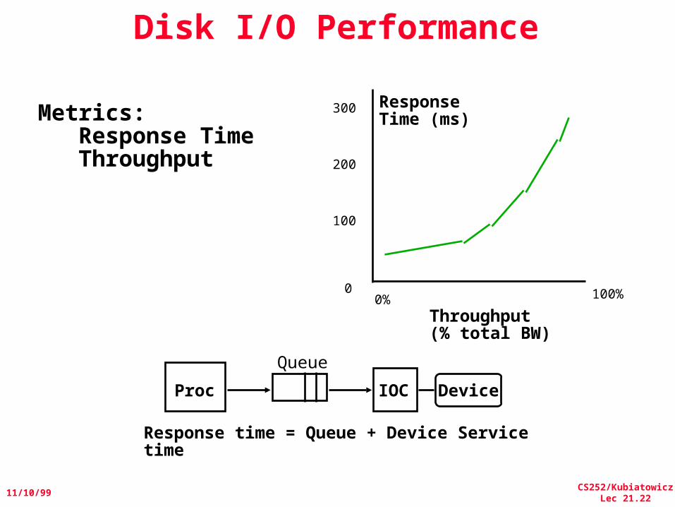
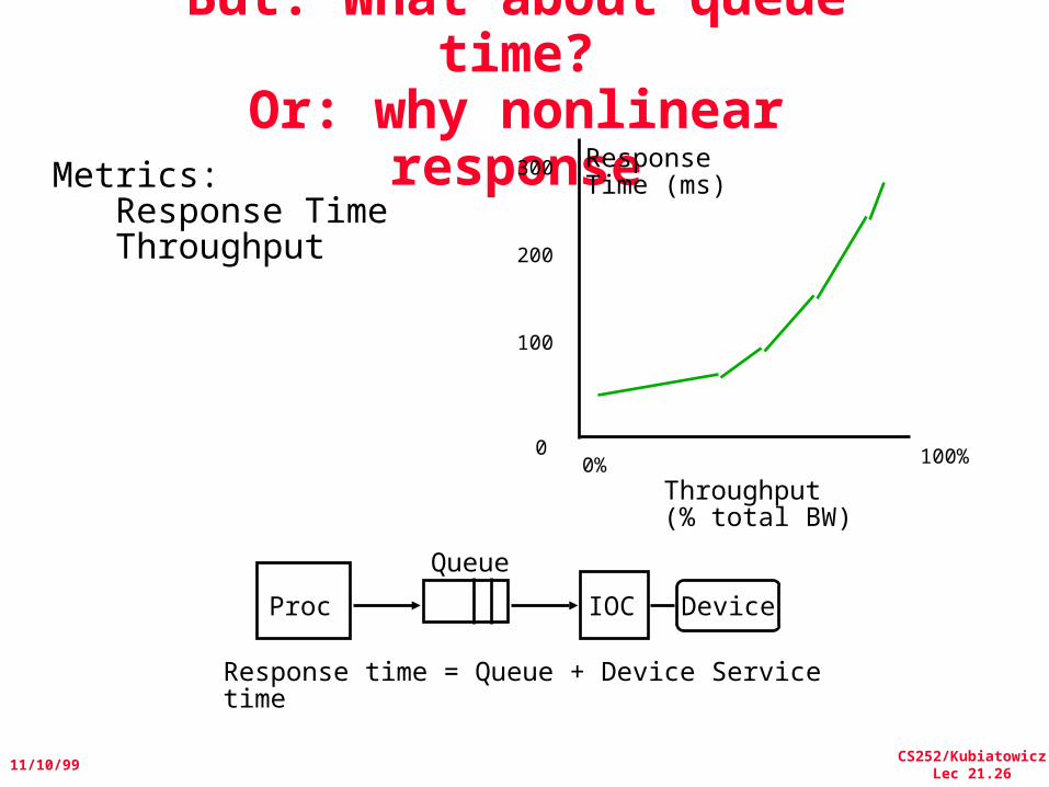
Disk I/O Performance

Response time = Queue + Device Service time

100%

ResponseTime (ms)

Throughput (% total BW)

0

100

200

300

0%

Proc

Queue

IOC Device

Metrics: Response Time Throughput


11/10/99

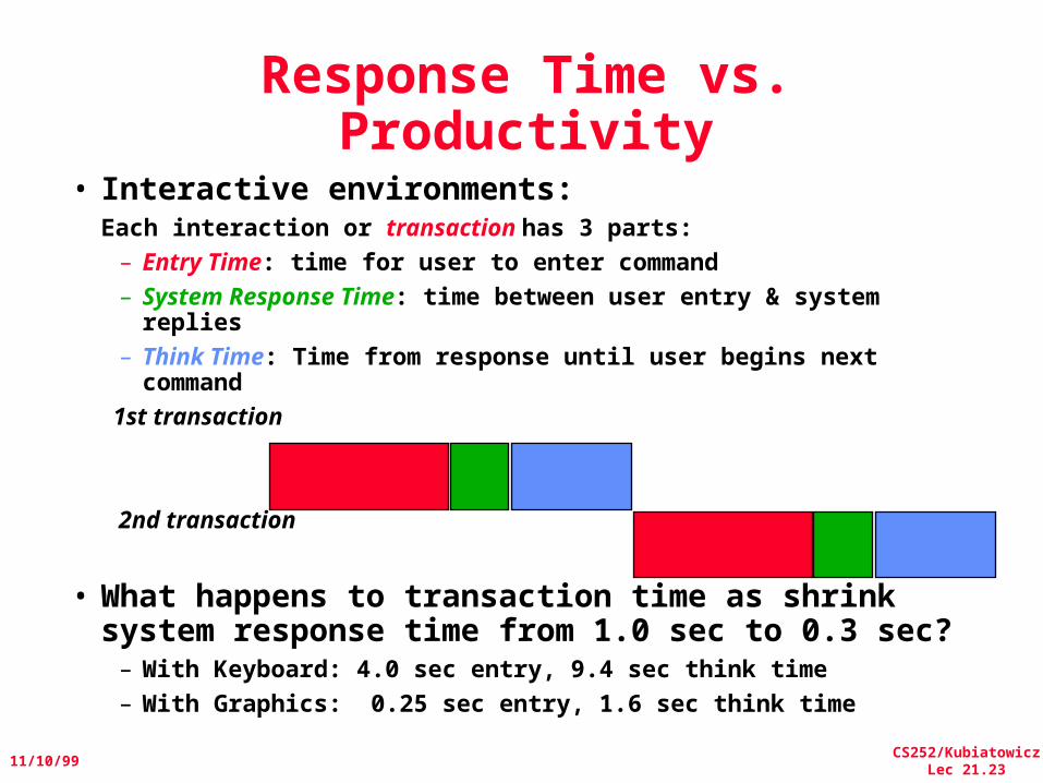
Response Time vs. Productivity

• Interactive environments: Each interaction or transaction has 3 parts:– Entry Time: time for user to enter command– System Response Time: time between user entry & system

replies– Think Time: Time from response until user begins next

command 1st transaction

2nd transaction

• What happens to transaction time as shrink system response time from 1.0 sec to 0.3 sec?– With Keyboard: 4.0 sec entry, 9.4 sec think time– With Graphics: 0.25 sec entry, 1.6 sec think time


11/10/99

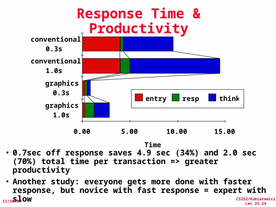
Time

0.00 5.00 10.00 15.00

graphics1.0s

graphics0.3s

conventional1.0s

conventional0.3s

entry resp think

Response Time & Productivity

• 0.7sec off response saves 4.9 sec (34%) and 2.0 sec (70%) total time per transaction => greater productivity

• Another study: everyone gets more done with faster response, but novice with fast response = expert with slow


11/10/99

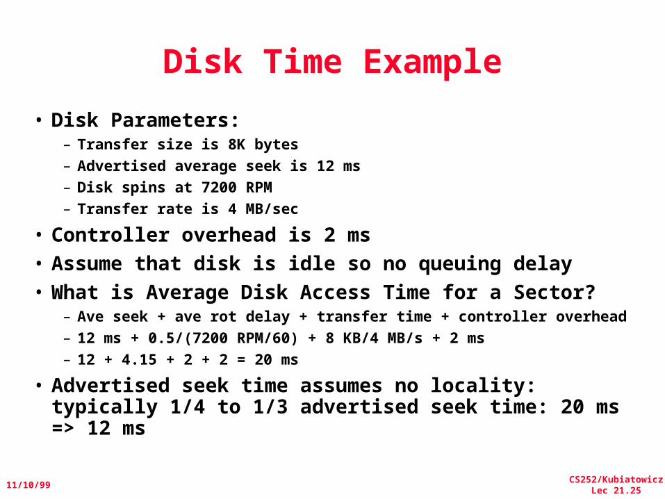
Disk Time Example

• Disk Parameters:– Transfer size is 8K bytes– Advertised average seek is 12 ms– Disk spins at 7200 RPM– Transfer rate is 4 MB/sec

• Controller overhead is 2 ms• Assume that disk is idle so no queuing delay• What is Average Disk Access Time for a Sector?

– Ave seek + ave rot delay + transfer time + controller overhead– 12 ms + 0.5/(7200 RPM/60) + 8 KB/4 MB/s + 2 ms– 12 + 4.15 + 2 + 2 = 20 ms

• Advertised seek time assumes no locality: typically 1/4 to 1/3 advertised seek time: 20 ms => 12 ms


11/10/99

But: What about queue time?

Or: why nonlinear response

Response time = Queue + Device Service time

100%

ResponseTime (ms)

Throughput (% total BW)

0

100

200

300

0%

Proc

Queue

IOC Device

Metrics: Response Time Throughput


11/10/99

Departure to discuss queueing theory

(On board)


11/10/99

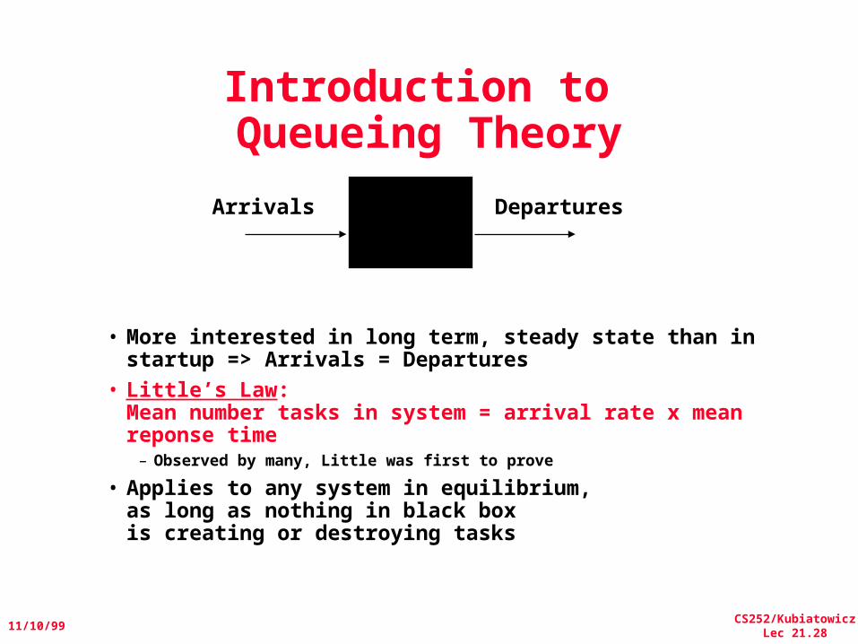
Introduction to Queueing Theory

• More interested in long term, steady state than in startup => Arrivals = Departures

• Little’s Law: Mean number tasks in system = arrival rate x mean reponse time– Observed by many, Little was first to prove

• Applies to any system in equilibrium, as long as nothing in black box is creating or destroying tasks

Arrivals Departures


11/10/99

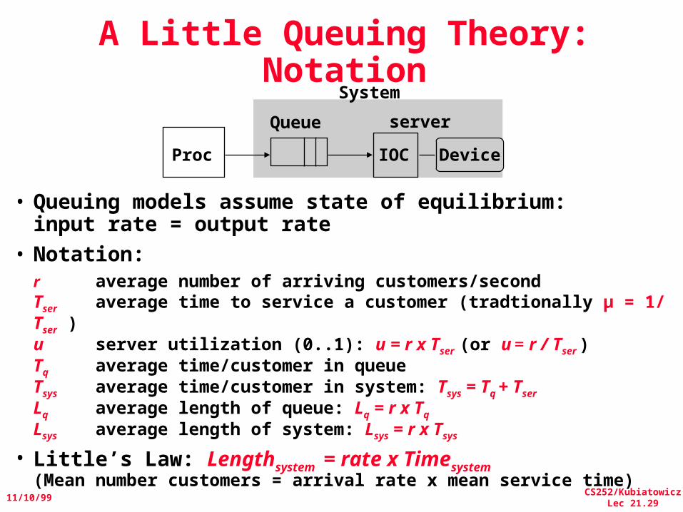
A Little Queuing Theory: Notation

• Queuing models assume state of equilibrium: input rate = output rate

• Notation: r average number of arriving customers/second

Tser average time to service a customer (tradtionally µ = 1/ Tser )u server utilization (0..1): u = r x Tser (or u = r / Tser )Tq average time/customer in queue Tsys average time/customer in system: Tsys = Tq + Tser

Lq average length of queue: Lq = r x Tq

Lsys average length of system: Lsys = r x Tsys

• Little’s Law: Lengthsystem = rate x Timesystem (Mean number customers = arrival rate x mean service time)

Proc IOC Device

Queue server

System


11/10/99

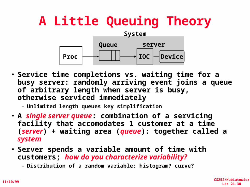
A Little Queuing Theory

• Service time completions vs. waiting time for a busy server: randomly arriving event joins a queue of arbitrary length when server is busy, otherwise serviced immediately– Unlimited length queues key simplification

• A single server queue: combination of a servicing facility that accomodates 1 customer at a time (server) + waiting area (queue): together called a system

• Server spends a variable amount of time with customers; how do you characterize variability?– Distribution of a random variable: histogram? curve?

Proc IOC Device

Queue server

System


11/10/99

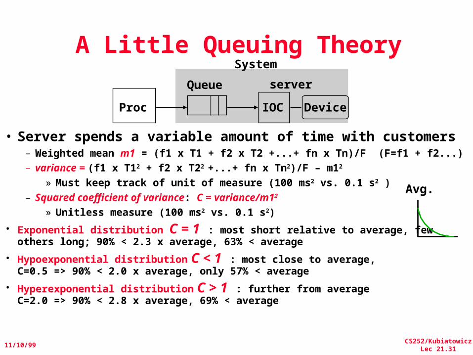
A Little Queuing Theory

• Server spends a variable amount of time with customers– Weighted mean m1 = (f1 x T1 + f2 x T2 +...+ fn x Tn)/F (F=f1 + f2...)– variance = (f1 x T12 + f2 x T22 +...+ fn x Tn2)/F – m12

» Must keep track of unit of measure (100 ms2 vs. 0.1 s2 )– Squared coefficient of variance: C = variance/m12

» Unitless measure (100 ms2 vs. 0.1 s2)

• Exponential distribution C = 1 : most short relative to average, few others long; 90% < 2.3 x average, 63% < average

• Hypoexponential distribution C < 1 : most close to average, C=0.5 => 90% < 2.0 x average, only 57% < average

• Hyperexponential distribution C > 1 : further from average C=2.0 => 90% < 2.8 x average, 69% < average

Proc IOC Device

Queue server

System

Avg.


11/10/99

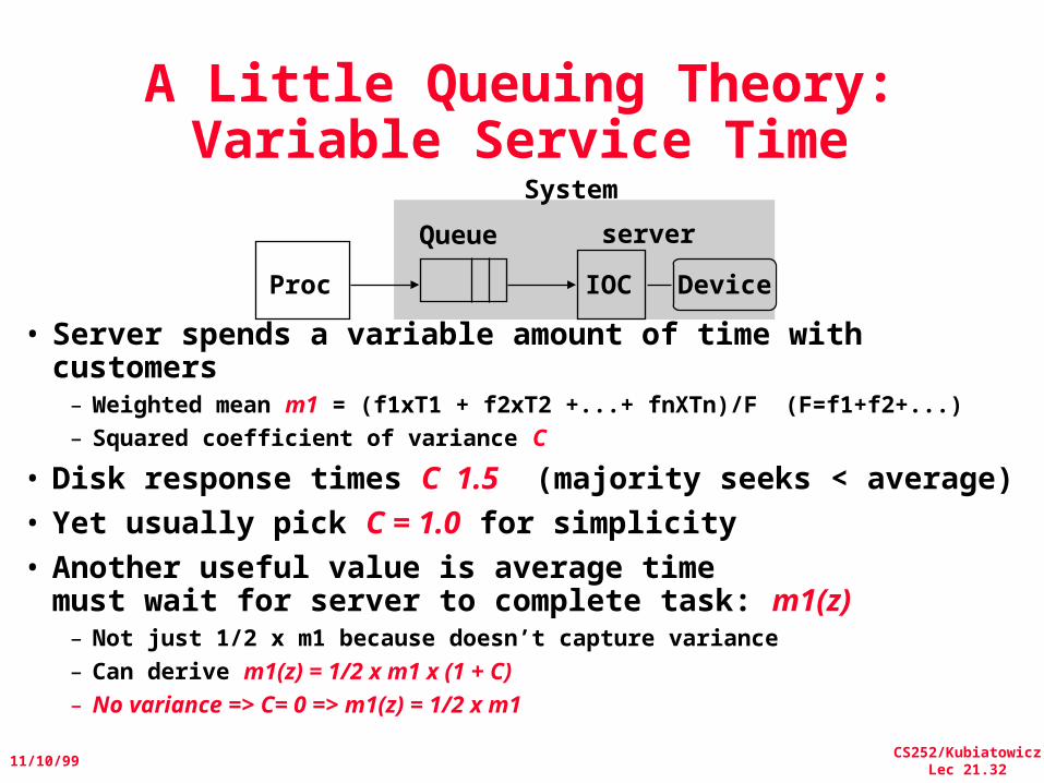
A Little Queuing Theory: Variable Service Time

• Server spends a variable amount of time with customers– Weighted mean m1 = (f1xT1 + f2xT2 +...+ fnXTn)/F (F=f1+f2+...)– Squared coefficient of variance C

• Disk response times C 1.5 (majority seeks < average)• Yet usually pick C = 1.0 for simplicity• Another useful value is average time

must wait for server to complete task: m1(z)– Not just 1/2 x m1 because doesn’t capture variance– Can derive m1(z) = 1/2 x m1 x (1 + C)– No variance => C= 0 => m1(z) = 1/2 x m1

Proc IOC Device

Queue server

System


11/10/99

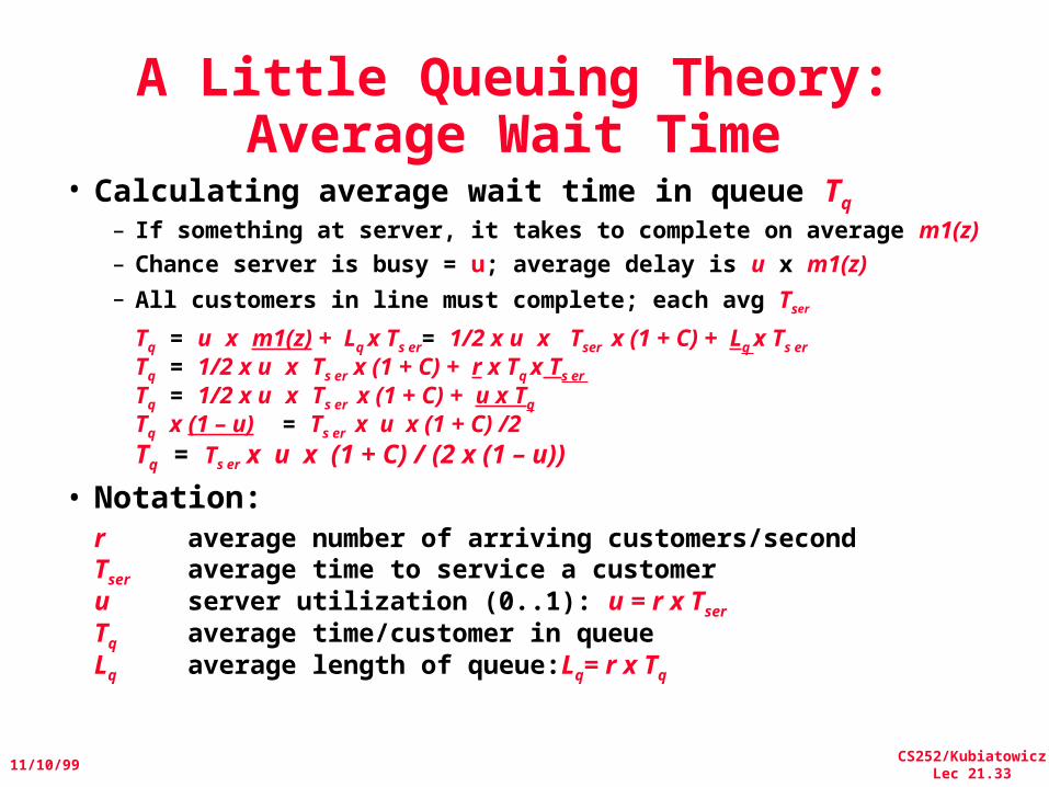
A Little Queuing Theory:Average Wait Time

• Calculating average wait time in queue Tq

– If something at server, it takes to complete on average m1(z)– Chance server is busy = u; average delay is u x m1(z)– All customers in line must complete; each avg Tser

Tq = u x m1(z) + Lq x Ts er= 1/2 x u x Tser x (1 + C) + Lq x Ts er

Tq = 1/2 x u x Ts er x (1 + C) + r x Tq x Ts er

Tq = 1/2 x u x Ts er x (1 + C) + u x Tq

Tq x (1 – u) = Ts er x u x (1 + C) /2Tq = Ts er x u x (1 + C) / (2 x (1 – u))

• Notation: r average number of arriving customers/second

Tser average time to service a customeru server utilization (0..1): u = r x Tser

Tq average time/customer in queueLq average length of queue:Lq= r x Tq


11/10/99

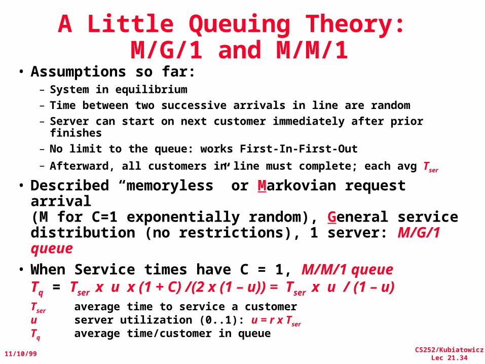
A Little Queuing Theory: M/G/1 and M/M/1

• Assumptions so far:– System in equilibrium– Time between two successive arrivals in line are random– Server can start on next customer immediately after prior

finishes– No limit to the queue: works First-In-First-Out

– Afterward, all customers in line must complete; each avg Tser

• Described “memoryless” or Markovian request arrival (M for C=1 exponentially random), General service distribution (no restrictions), 1 server: M/G/1 queue

• When Service times have C = 1, M/M/1 queueTq = Tser x u x (1 + C) /(2 x (1 – u)) = Tser x u / (1 – u)

Tser average time to service a customeru server utilization (0..1): u = r x Tser

Tq average time/customer in queue


11/10/99

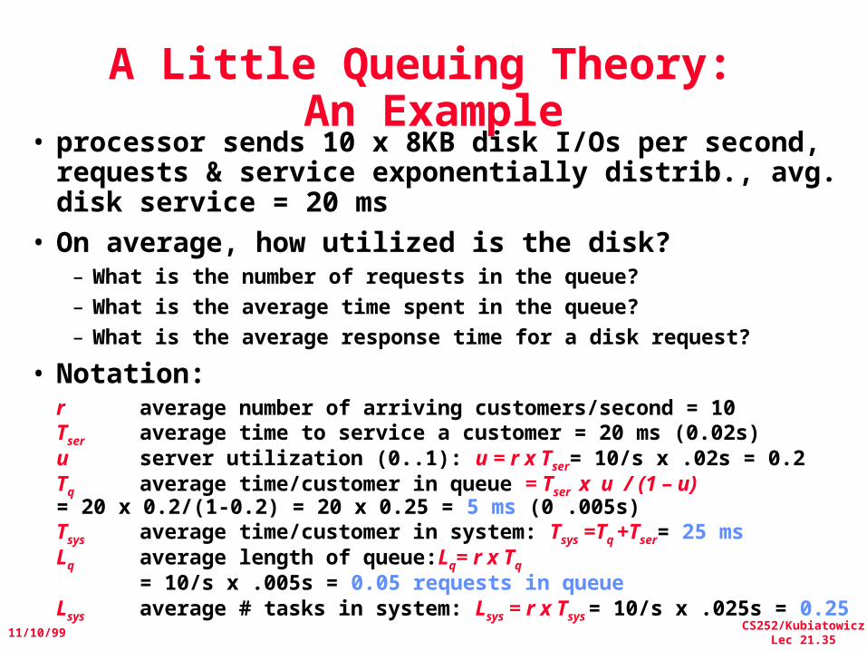
A Little Queuing Theory: An Example

• processor sends 10 x 8KB disk I/Os per second, requests & service exponentially distrib., avg. disk service = 20 ms

• On average, how utilized is the disk?– What is the number of requests in the queue?– What is the average time spent in the queue?– What is the average response time for a disk request?

• Notation: r average number of arriving customers/second = 10

Tser average time to service a customer = 20 ms (0.02s)u server utilization (0..1): u = r x Tser= 10/s x .02s = 0.2Tq average time/customer in queue = Tser x u / (1 – u)

= 20 x 0.2/(1-0.2) = 20 x 0.25 = 5 ms (0 .005s)Tsys average time/customer in system: Tsys =Tq +Tser= 25 msLq average length of queue:Lq= r x Tq

= 10/s x .005s = 0.05 requests in queueLsys average # tasks in system: Lsys = r x Tsys = 10/s x .025s = 0.25


11/10/99

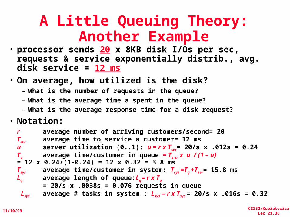
A Little Queuing Theory: Another Example

• processor sends 20 x 8KB disk I/Os per sec, requests & service exponentially distrib., avg. disk service = 12 ms

• On average, how utilized is the disk?– What is the number of requests in the queue?– What is the average time a spent in the queue?– What is the average response time for a disk request?

• Notation: r average number of arriving customers/second= 20

Tser average time to service a customer= 12 msu server utilization (0..1): u = r x Tser= 20/s x .012s = 0.24Tq average time/customer in queue = Ts er x u / (1 – u)

= 12 x 0.24/(1-0.24) = 12 x 0.32 = 3.8 msTsys average time/customer in system: Tsys =Tq +Tser= 15.8 msLq average length of queue:Lq= r x Tq

= 20/s x .0038s = 0.076 requests in queue Lsys average # tasks in system : Lsys = r x Tsys = 20/s x .016s = 0.32


11/10/99

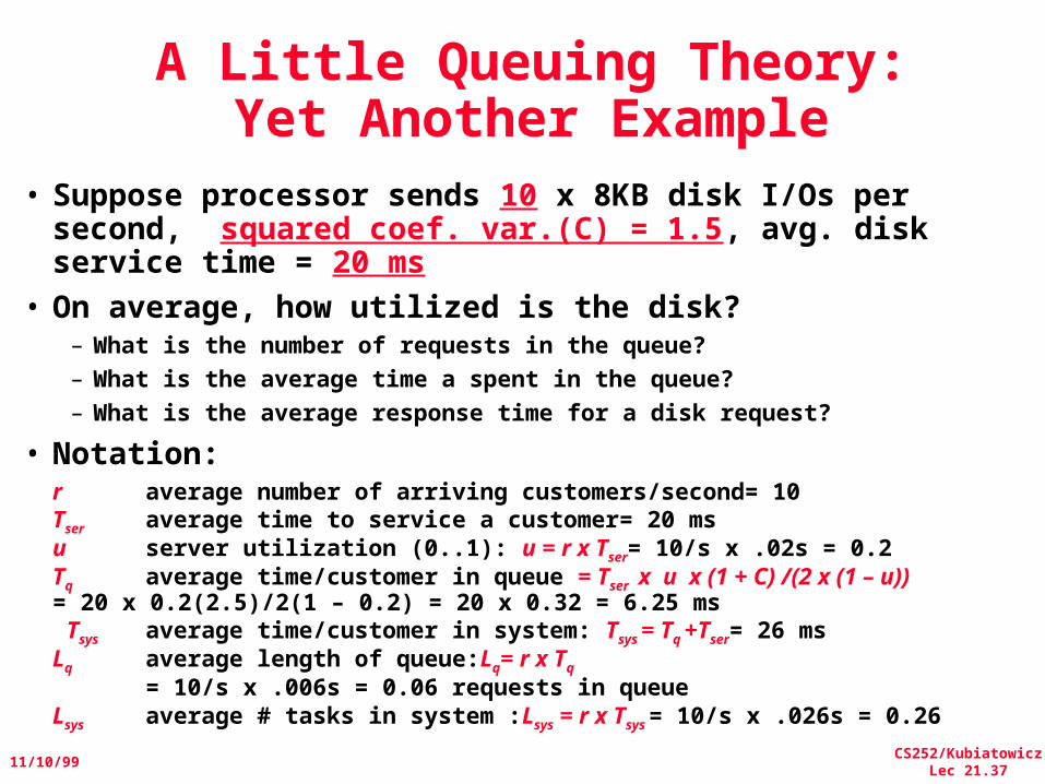
A Little Queuing Theory:Yet Another Example

• Suppose processor sends 10 x 8KB disk I/Os per second, squared coef. var.(C) = 1.5, avg. disk service time = 20 ms

• On average, how utilized is the disk?– What is the number of requests in the queue?– What is the average time a spent in the queue?– What is the average response time for a disk request?

• Notation: r average number of arriving customers/second= 10

Tser average time to service a customer= 20 msu server utilization (0..1): u = r x Tser= 10/s x .02s = 0.2Tq average time/customer in queue = Tser x u x (1 + C) /(2 x (1 – u))

= 20 x 0.2(2.5)/2(1 – 0.2) = 20 x 0.32 = 6.25 ms Tsys average time/customer in system: Tsys = Tq +Tser= 26 msLq average length of queue:Lq= r x Tq

= 10/s x .006s = 0.06 requests in queueLsys average # tasks in system :Lsys = r x Tsys = 10/s x .026s = 0.26


11/10/99

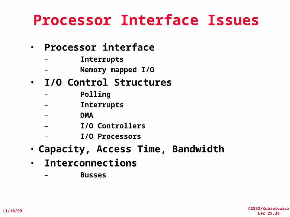
Processor Interface Issues

• Processor interface– Interrupts– Memory mapped I/O

• I/O Control Structures– Polling– Interrupts– DMA– I/O Controllers– I/O Processors

• Capacity, Access Time, Bandwidth• Interconnections

– Busses


11/10/99

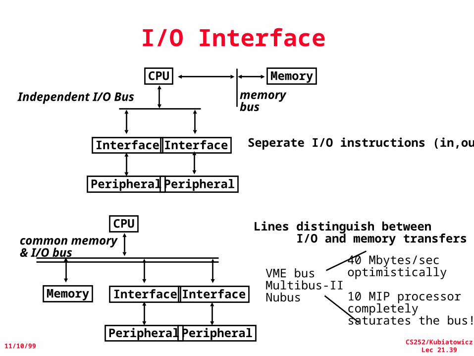
I/O Interface

Independent I/O Bus

CPU

Interface Interface

Peripheral Peripheral

Memory

memorybus

Seperate I/O instructions (in,out)

CPU

Interface Interface


Memory

Lines distinguish between I/O and memory transferscommon memory

& I/O bus

VME busMultibus-IINubus

40 Mbytes/secoptimistically

10 MIP processorcompletelysaturates the bus!


11/10/99

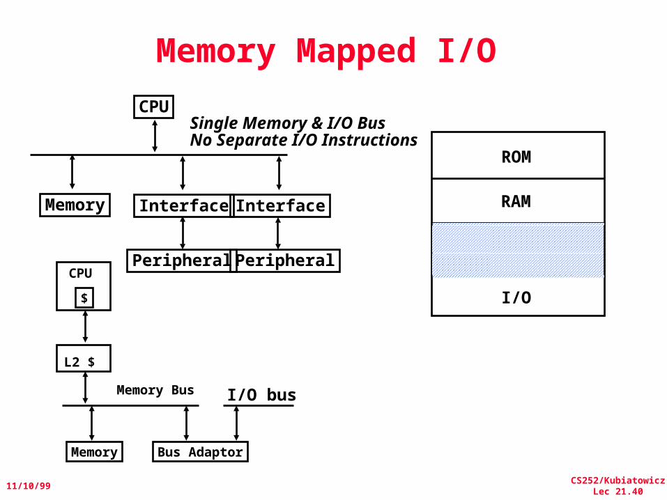
Memory Mapped I/O

Single Memory & I/O Bus No Separate I/O Instructions

CPU

Interface Interface


Memory

ROM

RAM

I/O$

CPU

L2 $

Memory Bus

Memory Bus Adaptor

I/O bus


11/10/99

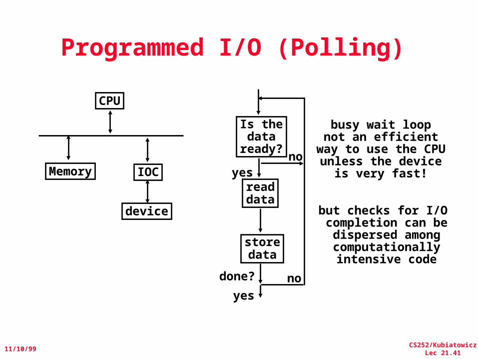
Programmed I/O (Polling)

CPU

IOC

device

Memory

Is thedata

ready?

readdata

storedata

yesno

done? no

yes

busy wait loopnot an efficient

way to use the CPUunless the device

is very fast!

but checks for I/O completion can bedispersed amongcomputationallyintensive code


11/10/99

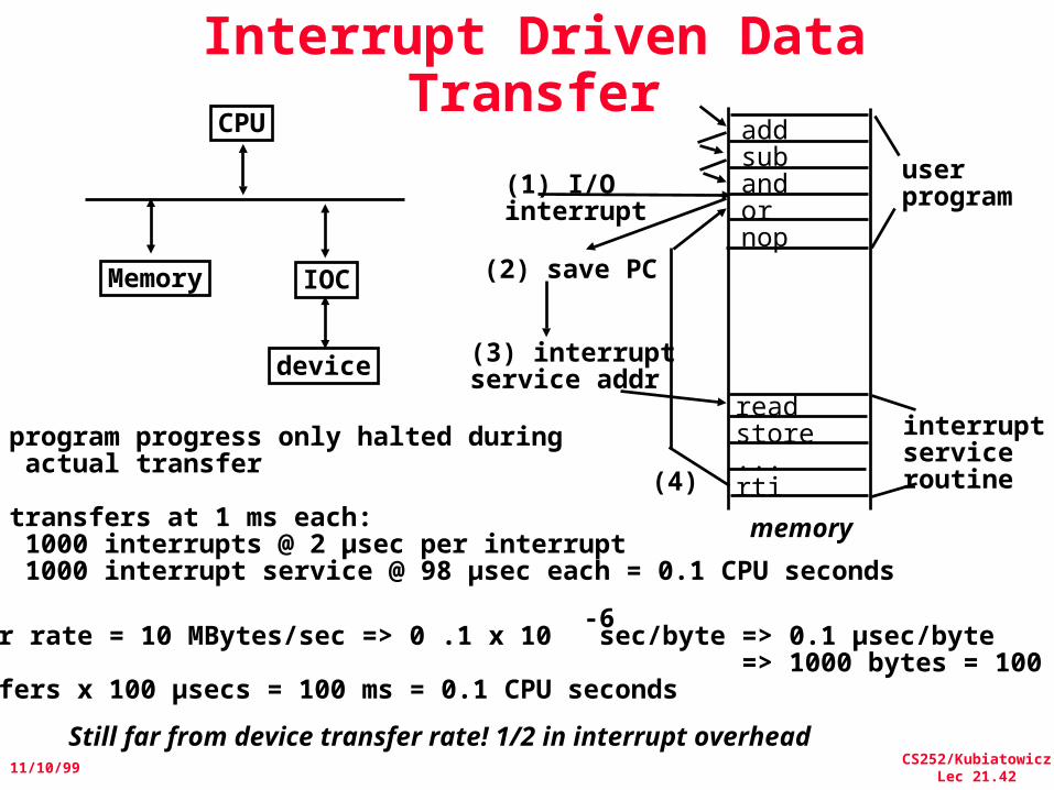
Interrupt Driven Data TransferCPU

IOC

device

Memory

addsubandornop

readstore...rti

memory

userprogram(1) I/O

interrupt

(2) save PC

(3) interruptservice addr

interruptserviceroutine(4)

Device xfer rate = 10 MBytes/sec => 0 .1 x 10 sec/byte => 0.1 µsec/byte => 1000 bytes = 100 µsec 1000 transfers x 100 µsecs = 100 ms = 0.1 CPU seconds

-6

User program progress only halted during actual transfer

1000 transfers at 1 ms each: 1000 interrupts @ 2 µsec per interrupt 1000 interrupt service @ 98 µsec each = 0.1 CPU seconds

Still far from device transfer rate! 1/2 in interrupt overhead


11/10/99

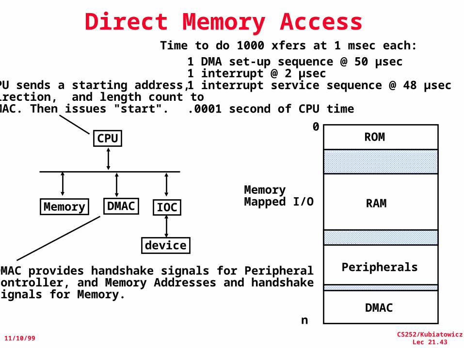
Direct Memory Access

CPU

IOC

device

Memory DMAC

Time to do 1000 xfers at 1 msec each:1 DMA set-up sequence @ 50 µsec1 interrupt @ 2 µsec1 interrupt service sequence @ 48 µsec

.0001 second of CPU time

CPU sends a starting address, direction, and length count to DMAC. Then issues "start".

DMAC provides handshake signals for PeripheralController, and Memory Addresses and handshakesignals for Memory.

0ROM

RAM

Peripherals

DMACn

Memory Mapped I/O


11/10/99

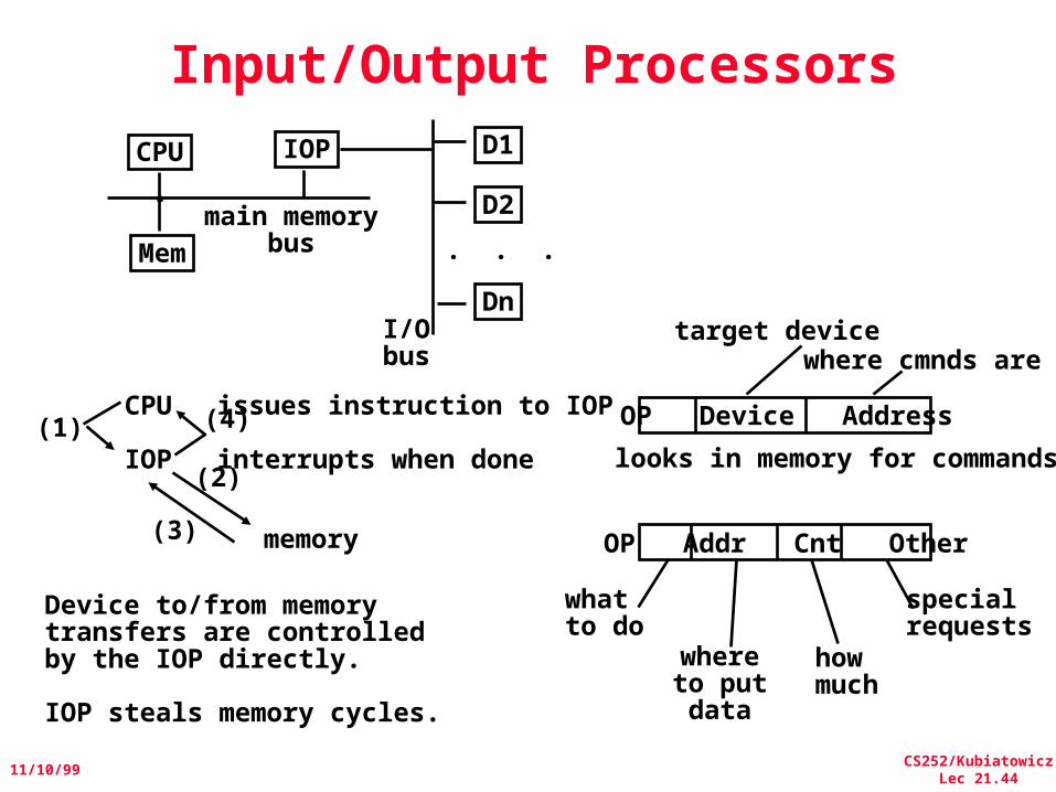
Input/Output Processors

CPU IOP

Mem

D1

D2

Dn

. . .main memory

bus

I/Obus

CPU

IOP

issues instruction to IOP

interrupts when done(1)

memory

(2)

(3)

(4)

Device to/from memorytransfers are controlledby the IOP directly.

IOP steals memory cycles.

OP Device Address

target devicewhere cmnds are

looks in memory for commands

OP Addr Cnt Other

whatto do

whereto putdata

howmuch

specialrequests


11/10/99

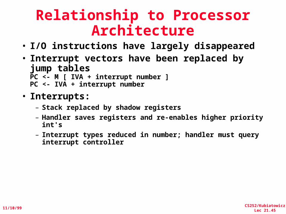
Relationship to Processor Architecture

• I/O instructions have largely disappeared• Interrupt vectors have been replaced by

jump tablesPC <- M [ IVA + interrupt number ]PC <- IVA + interrupt number

• Interrupts:– Stack replaced by shadow registers– Handler saves registers and re-enables higher priority

int's– Interrupt types reduced in number; handler must query

interrupt controller


11/10/99

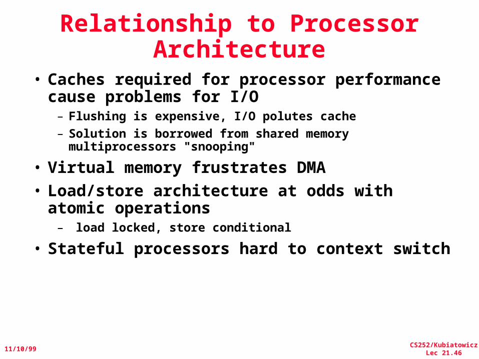
Relationship to Processor Architecture

• Caches required for processor performance cause problems for I/O– Flushing is expensive, I/O polutes cache– Solution is borrowed from shared memory

multiprocessors "snooping"

• Virtual memory frustrates DMA• Load/store architecture at odds with atomic

operations– load locked, store conditional

• Stateful processors hard to context switch


11/10/99

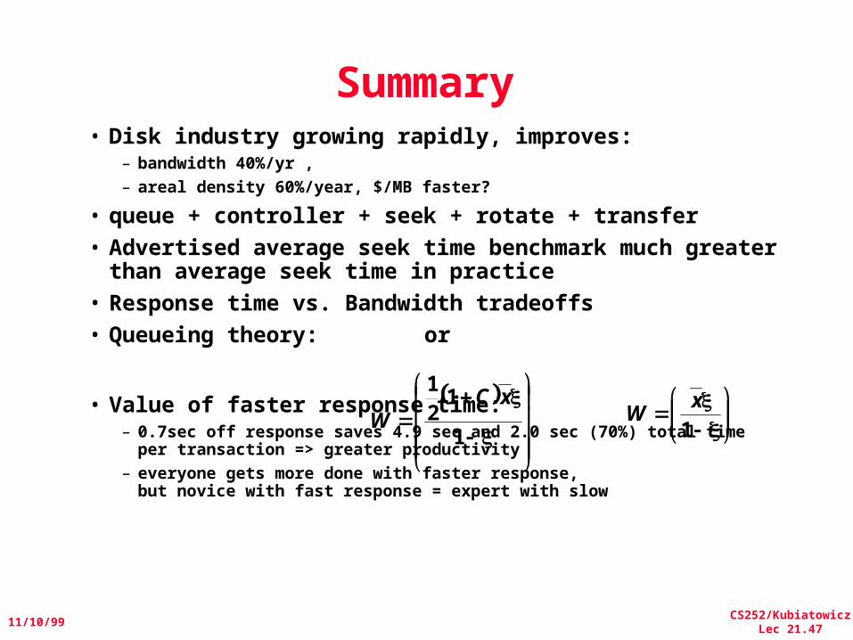
Summary• Disk industry growing rapidly, improves:

– bandwidth 40%/yr , – areal density 60%/year, $/MB faster?

• queue + controller + seek + rotate + transfer• Advertised average seek time benchmark much

greater than average seek time in practice• Response time vs. Bandwidth tradeoffs• Queueing theory: or

• Value of faster response time:– 0.7sec off response saves 4.9 sec and 2.0 sec (70%) total time

per transaction => greater productivity– everyone gets more done with faster response,

but novice with fast response = expert with slow

1

121

xCW

1

xW


11/10/99

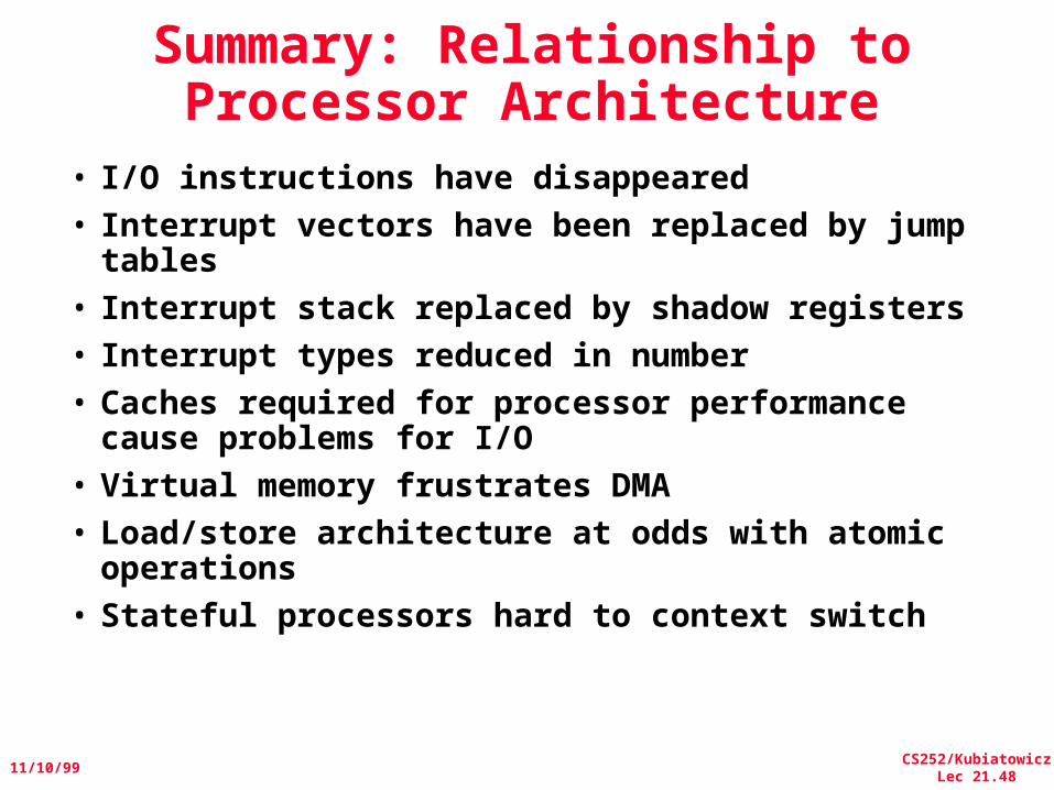
Summary: Relationship to Processor Architecture

• I/O instructions have disappeared• Interrupt vectors have been replaced by jump

tables• Interrupt stack replaced by shadow registers• Interrupt types reduced in number• Caches required for processor performance

cause problems for I/O• Virtual memory frustrates DMA• Load/store architecture at odds with atomic

operations• Stateful processors hard to context switch

Documents

CS252/Kubiatowicz Lec 21.1 11/10/99 CS252 Graduate Computer Architecture Lecture 21 I/O Introduction Prof. John Kubiatowicz Computer Science 252 Fall 1998