Embed Size (px)
Citation preview
CS407 Neural Computation
Lecture 3: Neural NetworkLearning Rules
Lecturer: A/Prof. M. Bennamoun
Learning--DefinitionLearning is a process by which free parameters of NN are adapted thru stimulation from environmentSequence of Events– stimulated by an environment– undergoes changes in its free parameters– responds in a new way to the environment
Learning Algorithm– prescribed steps of process to make a system
learn• ways to adjust synaptic weight of a neuron
– No unique learning algorithms - kit of toolsThe Lecture covers– five learning rules, learning paradigms– probabilistic and statistical aspect of learning
Review:
Gradients and DerivativesGradient Descent Minimization
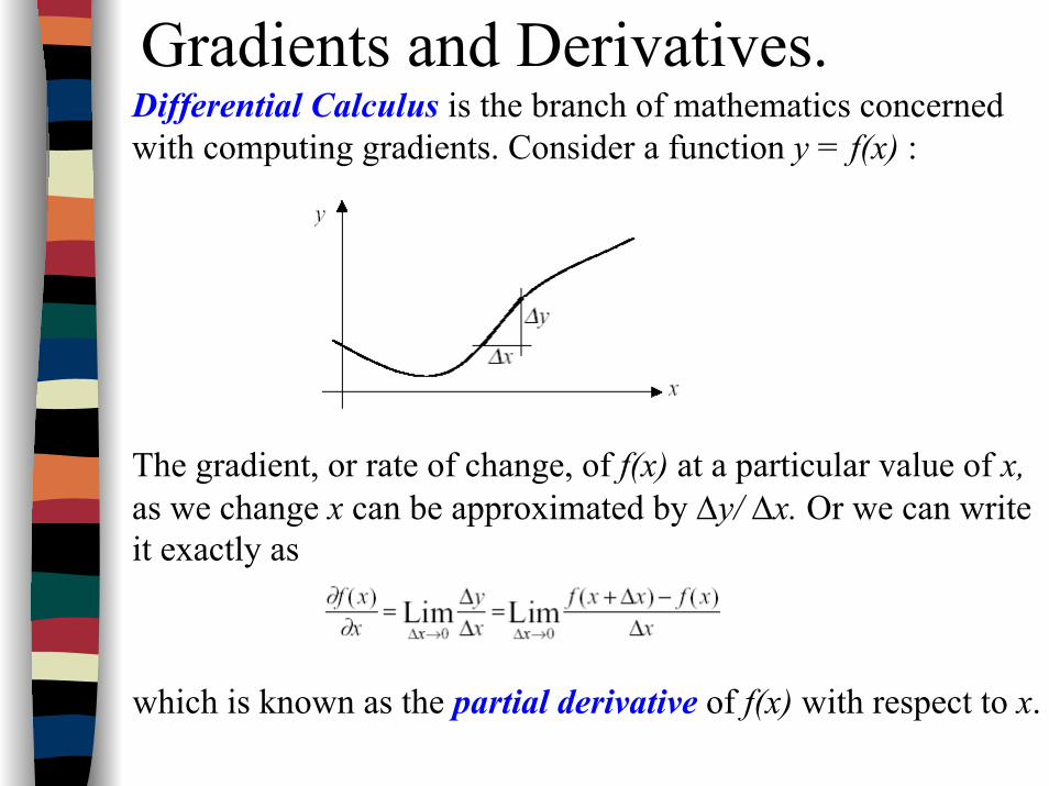
Gradients and Derivatives.Differential Calculus is the branch of mathematics concerned with computing gradients. Consider a function y = f(x) :
The gradient, or rate of change, of f(x) at a particular value of x, as we change x can be approximated by ∆y/ ∆x. Or we can write it exactly as
which is known as the partial derivative of f(x) with respect to x.
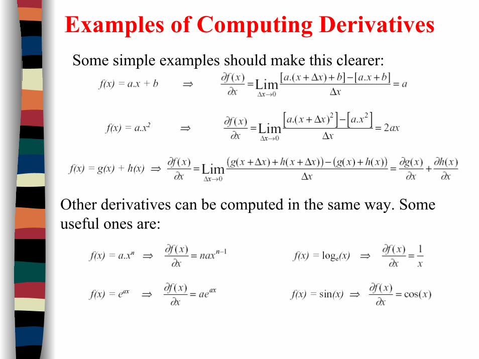
Examples of Computing DerivativesSome simple examples should make this clearer:
Other derivatives can be computed in the same way. Some useful ones are:
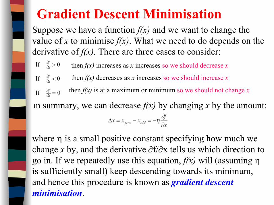
Gradient Descent MinimisationSuppose we have a function f(x) and we want to change the value of x to minimise f(x). What we need to do depends on the derivative of f(x). There are three cases to consider:
then f(x) increases as x increases so we should decrease x
then f(x) decreases as x increases so we should increase x
then f(x) is at a maximum or minimum so we should not change x
In summary, we can decrease f(x) by changing x by the amount:
where η is a small positive constant specifying how much we change x by, and the derivative ∂f/∂x tells us which direction to go in. If we repeatedly use this equation, f(x) will (assuming η is sufficiently small) keep descending towards its minimum, and hence this procedure is known as gradient descent minimisation.
Types of Learning
Learning with Teacher
Supervised learningTeacher has knowledge of environment to learninput and desired output pairs are given as a training setParameters are adjusted based on error signalstep-by-step– The desired response of the system is provided
by a teacher, e.g., the distance ρ[d,o] as an error measure

Learning with Teacher

Learning with Teacher– Estimate the negative error gradient direction and reduce the
error accordingly• Modify the synaptic weights to reduce the stochastic
minimization of error in multidimensional weight spaceMove toward a minimum point of error surface– may not be a global minimum– use gradient of error surface - direction of steepest descent
Good for pattern recognition and function approximation
Unsupervised LearningSelf-organized learning– The desired response is unknown, no explicit error
information can be used to improve network behavior
• E.g. finding the cluster boundaries of input patterns
– Suitable weight self-adaptation mechanisms have to be embedded in the trained network
– No external teacher or critics– Task-independent measure of quality is required
to learn– Network parameters are optimized with respect to
a measure– competitive learning rule is a case of unsupervised
learning
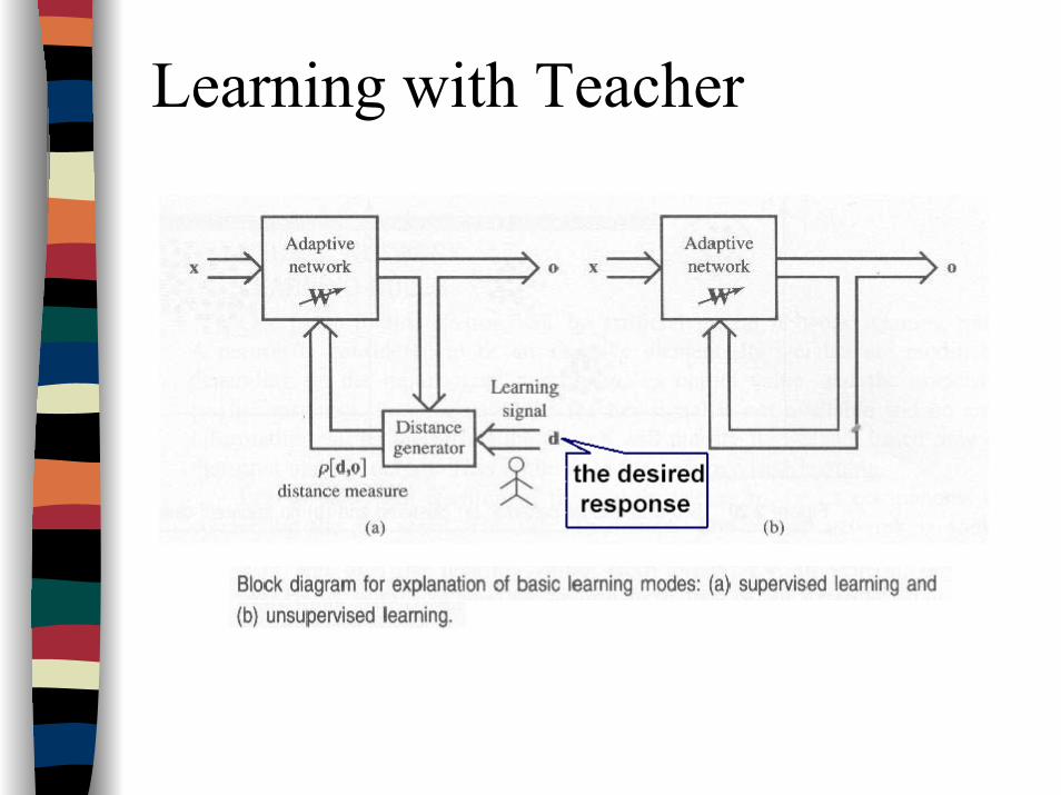
Learning with Teacher
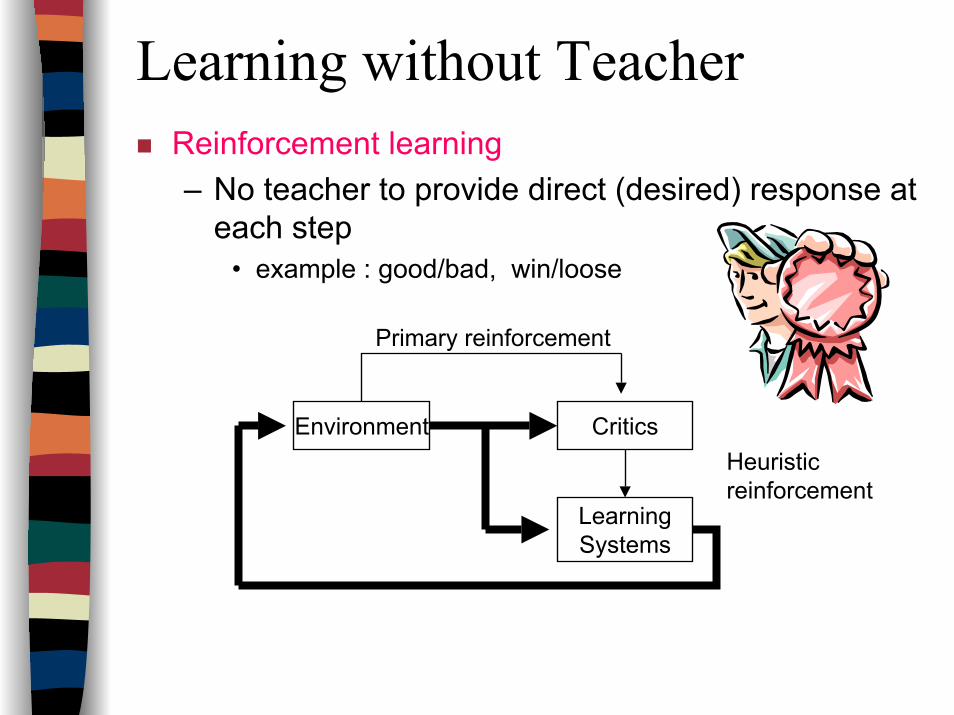
Learning without TeacherReinforcement learning– No teacher to provide direct (desired) response at
each step• example : good/bad, win/loose
Environment Critics
LearningSystems
Primary reinforcement
Heuristicreinforcement
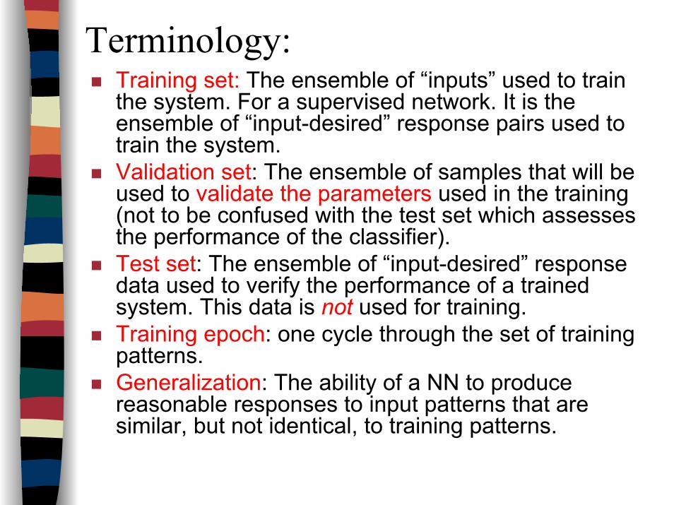
Terminology:Training set: The ensemble of “inputs” used to train the system. For a supervised network. It is the ensemble of “input-desired” response pairs used to train the system.Validation set: The ensemble of samples that will be used to validate the parameters used in the training (not to be confused with the test set which assesses the performance of the classifier).Test set: The ensemble of “input-desired” response data used to verify the performance of a trained system. This data is not used for training.Training epoch: one cycle through the set of training patterns.Generalization: The ability of a NN to produce reasonable responses to input patterns that are similar, but not identical, to training patterns.
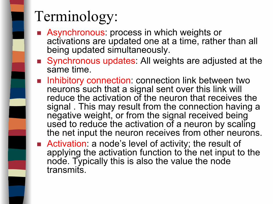
Terminology:Asynchronous: process in which weights or activations are updated one at a time, rather than all being updated simultaneously.Synchronous updates: All weights are adjusted at the same time.Inhibitory connection: connection link between two neurons such that a signal sent over this link will reduce the activation of the neuron that receives the signal . This may result from the connection having a negative weight, or from the signal received being used to reduce the activation of a neuron by scaling the net input the neuron receives from other neurons.Activation: a node’s level of activity; the result of applying the activation function to the net input to the node. Typically this is also the value the node transmits.

Review:
Vectors- Overview

Vectors- A Brief review
2-D vector Vector w.r.t cartesian axes
22
21 vvv +=
r
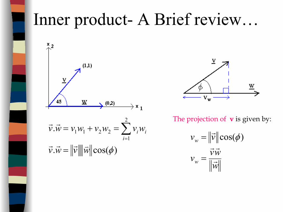
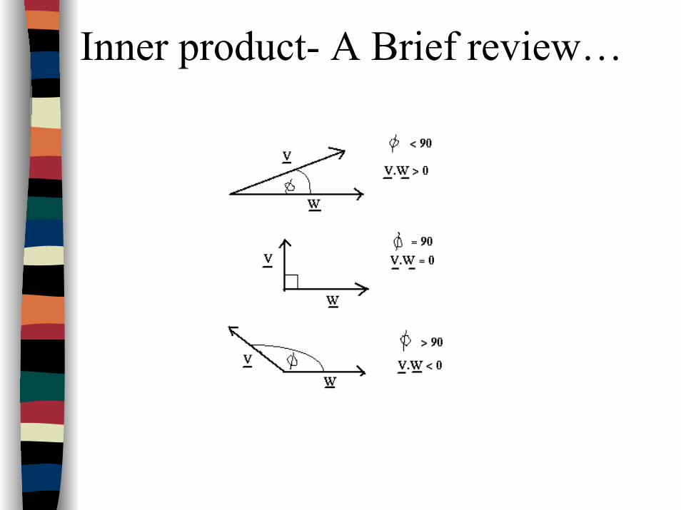
Inner product- A Brief review…
)cos(.
.2
12211
φwvwv
wvwvwvwvi
ii
vrrr
rr
=
=+= ∑=
The projection of v is given by:
wwvv
vv
w
w
r
rr
r
=
= )cos(φ
Inner product- A Brief review…
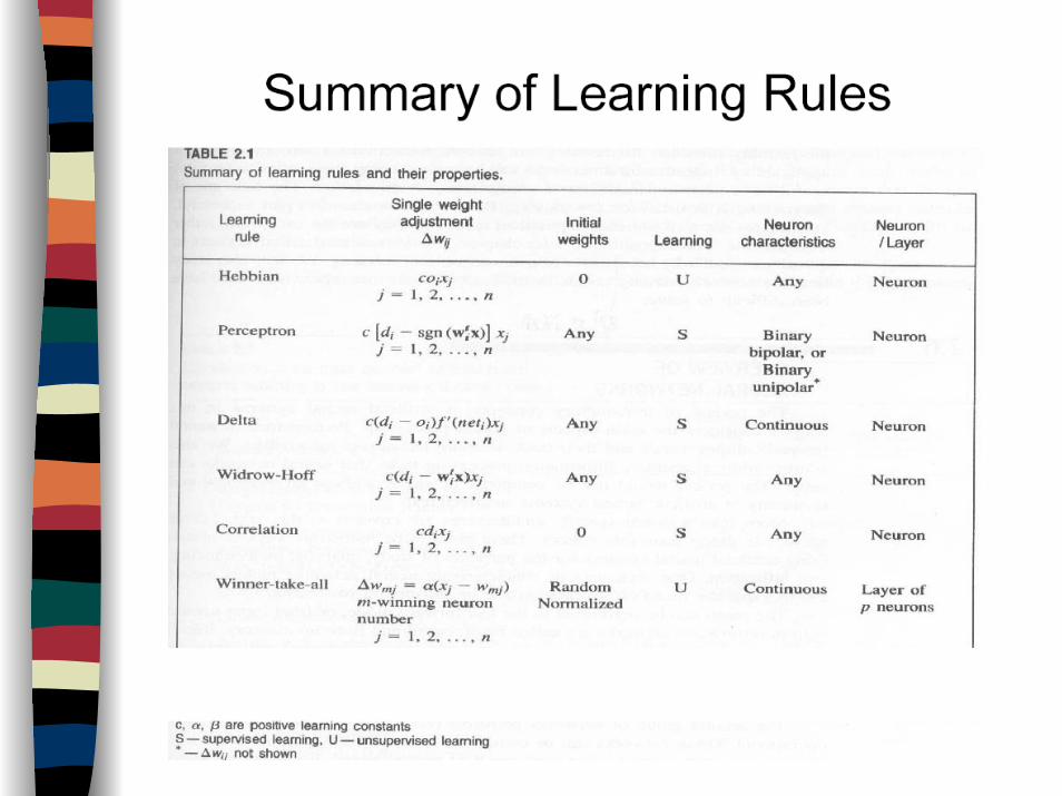
Learning Rules (LR)
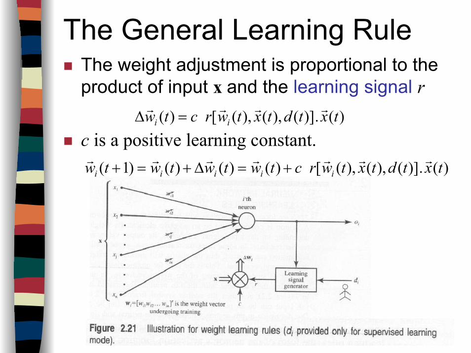
The General Learning RuleThe weight adjustment is proportional to the product of input x and the learning signal r
c is a positive learning constant.)(.)](),(),([)( txtdtxtwrctw ii
rrrr=∆
)(.)](),(),([)()()()1( txtdtxtwrctwtwtwtw iiiiirrrrrrr
+=∆+=+
Learning Rule 1
Error Correction Learning Rule
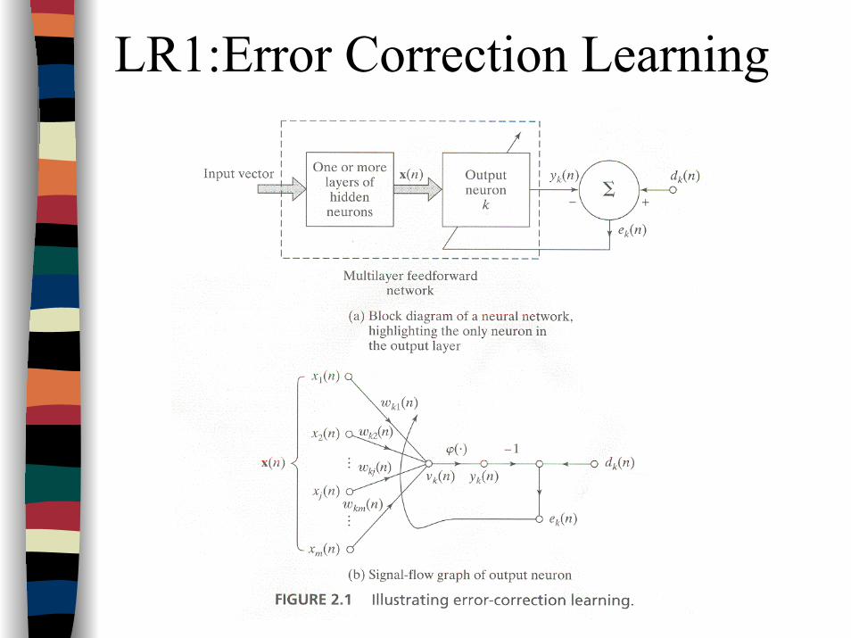
LR1:Error Correction Learning
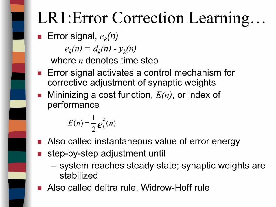
LR1:Error Correction Learning…Error signal, ek(n)
ek(n) = dk(n) - yk(n)where n denotes time step
Error signal activates a control mechanism for corrective adjustment of synaptic weightsMininizing a cost function, E(n), or index of performance
Also called instantaneous value of error energystep-by-step adjustment until– system reaches steady state; synaptic weights are
stabilizedAlso called deltra rule, Widrow-Hoff rule
)(21)( 2 nnE ek=
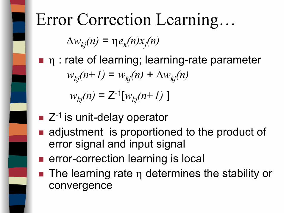
Error Correction Learning…∆wkj(n) = ηek(n)xj(n)
η : rate of learning; learning-rate parameterwkj(n+1) = wkj(n) + ∆wkj(n)
wkj(n) = Z-1[wkj(n+1) ]
Z-1 is unit-delay operatoradjustment is proportioned to the product of error signal and input signalerror-correction learning is localThe learning rate η determines the stability or convergence

E.g 1: Perceptron Learning RuleSupervised learning, only applicable for binary neuron
response (e.g. [-1,1])
The learning signal is equal to:
E.g., in classification task, the weight is adapted only when classification error occurred
The weight initialisation is random
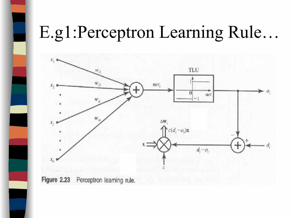
E.g1:Perceptron Learning Rule…
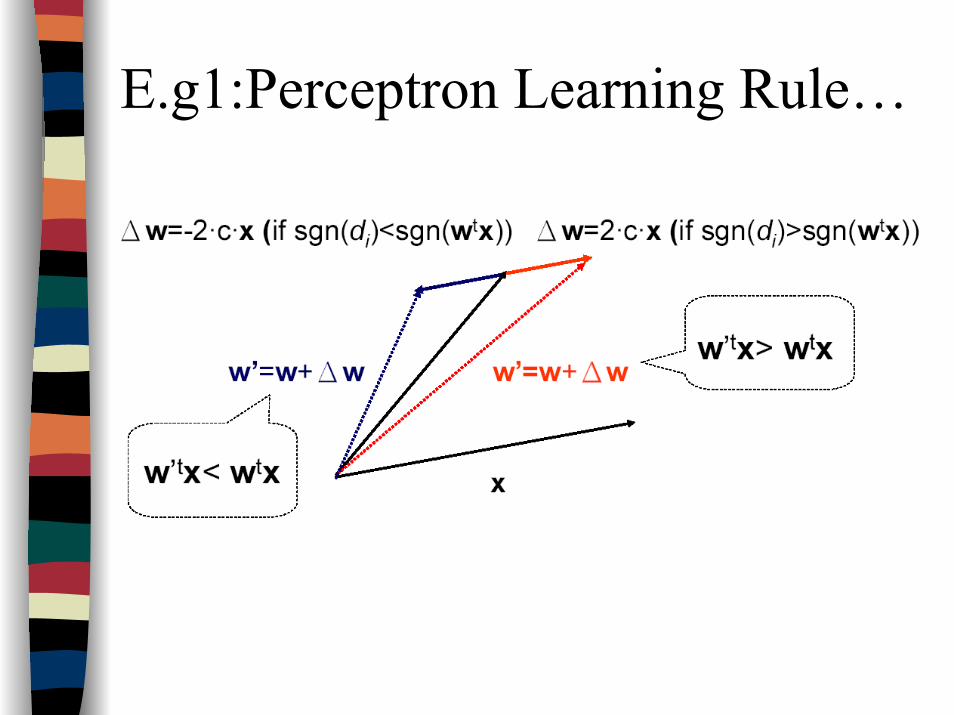
E.g1:Perceptron Learning Rule…
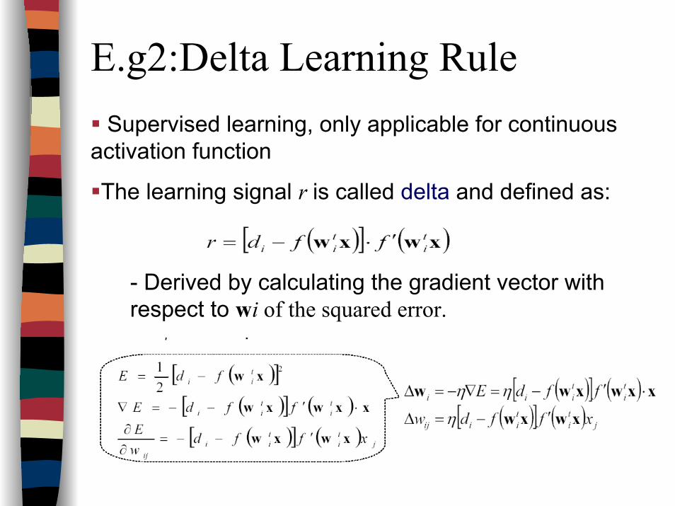
E.g2:Delta Learning RuleSupervised learning, only applicable for continuous
activation function
The learning signal r is called delta and defined as:
- Derived by calculating the gradient vector with respect to wi of the squared error.
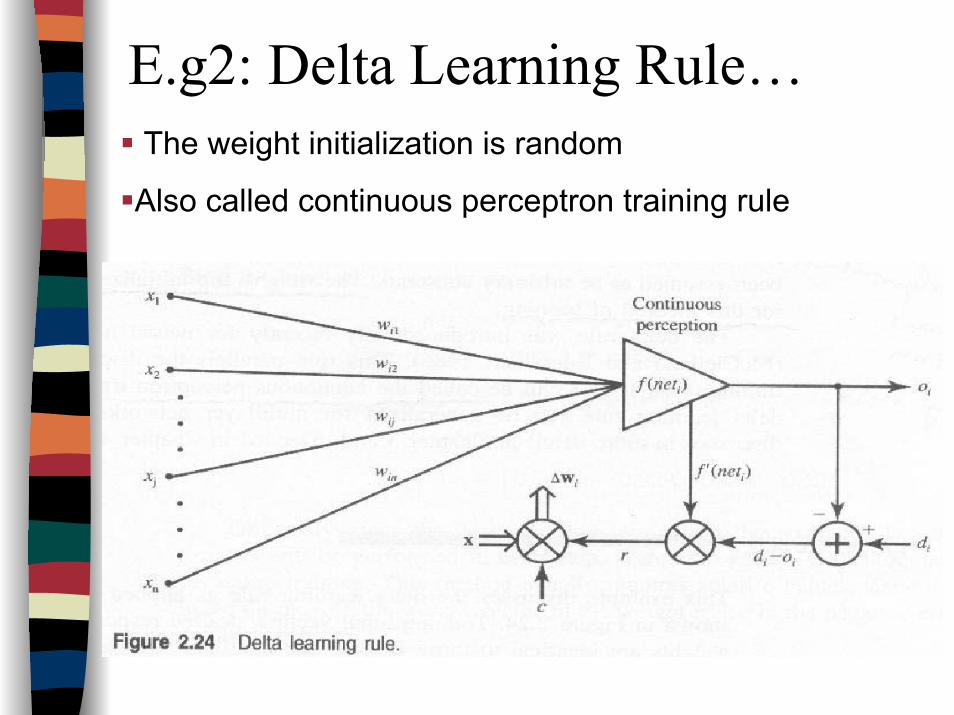
E.g2: Delta Learning Rule…The weight initialization is random
Also called continuous perceptron training rule
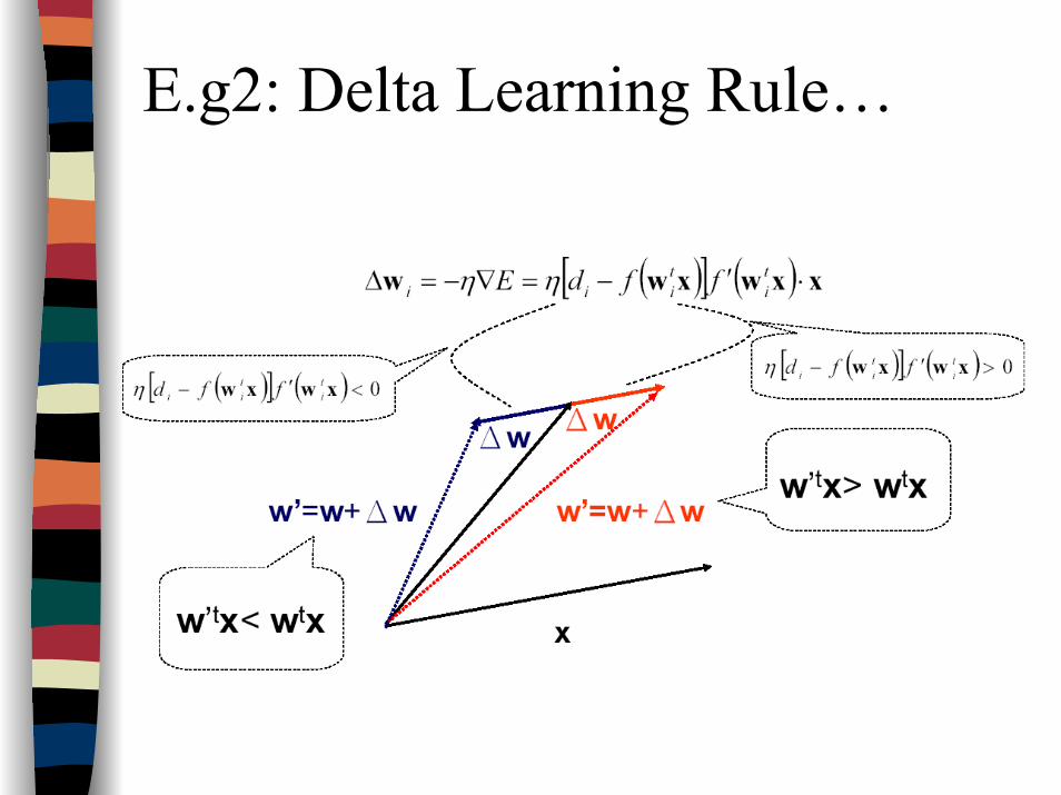
E.g2: Delta Learning Rule…
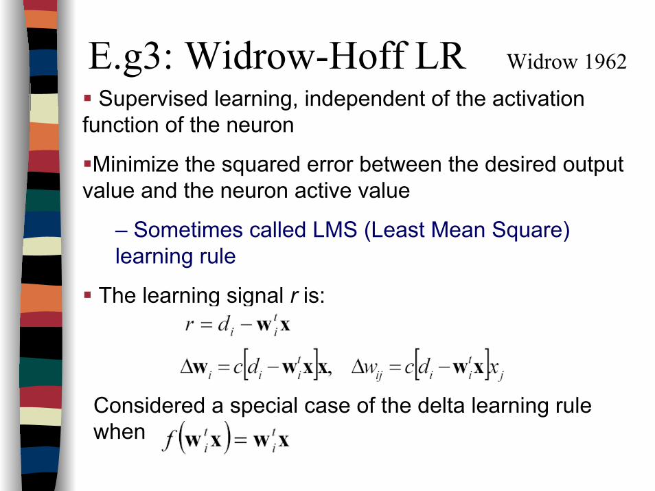
E.g3: Widrow-Hoff LR Widrow 1962
Supervised learning, independent of the activation function of the neuron
Minimize the squared error between the desired output value and the neuron active value
– Sometimes called LMS (Least Mean Square) learning rule
The learning signal r is:
Considered a special case of the delta learning rule when
Learning Rule 2
Memory-based Learning Rule
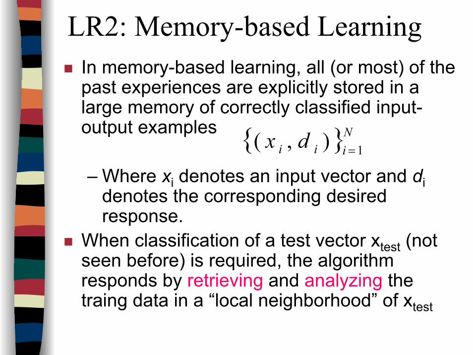
LR2: Memory-based LearningIn memory-based learning, all (or most) of the past experiences are explicitly stored in a large memory of correctly classified input-output examples
– Where xi denotes an input vector and didenotes the corresponding desired response.
When classification of a test vector xtest (not seen before) is required, the algorithm responds by retrieving and analyzing the traing data in a “local neighborhood” of xtest
{ }Niii dx 1),( =
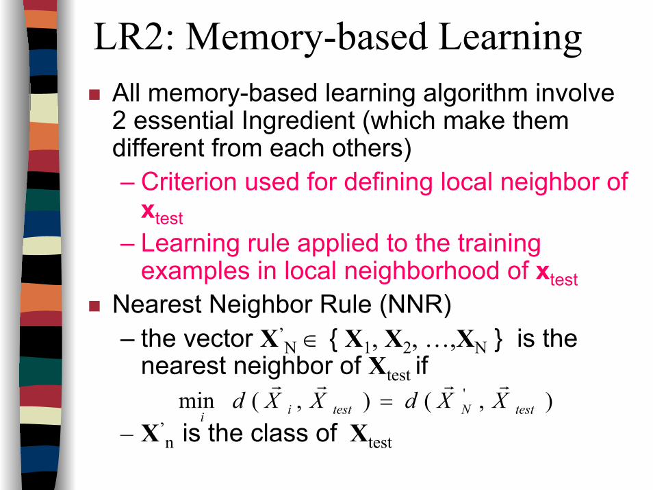
LR2: Memory-based LearningAll memory-based learning algorithm involve 2 essential Ingredient (which make them different from each others)– Criterion used for defining local neighbor of
xtest– Learning rule applied to the training
examples in local neighborhood of xtestNearest Neighbor Rule (NNR)– the vector X’
N ∈ { X1, X2, …,XN } is the nearest neighbor of Xtest if
– X’n is the class of Xtest
),(),(min 'testNtestii
XXdXXdrrrr
=
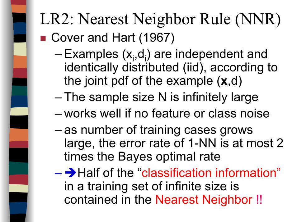
LR2: Nearest Neighbor Rule (NNR)Cover and Hart (1967)– Examples (xi,di) are independent and
identically distributed (iid), according to the joint pdf of the example (x,d)
– The sample size N is infinitely large– works well if no feature or class noise– as number of training cases grows
large, the error rate of 1-NN is at most 2 times the Bayes optimal rate
– Half of the “classification information”in a training set of infinite size is contained in the Nearest Neighbor !!
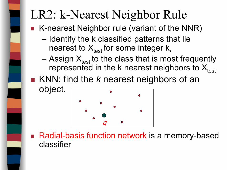
LR2: k-Nearest Neighbor RuleK-nearest Neighbor rule (variant of the NNR)– Identify the k classified patterns that lie
nearest to Xtest for some integer k, – Assign Xtest to the class that is most frequently
represented in the k nearest neighbors to Xtest
KNN: find the k nearest neighbors of an object.
Radial-basis function network is a memory-based classifier
q
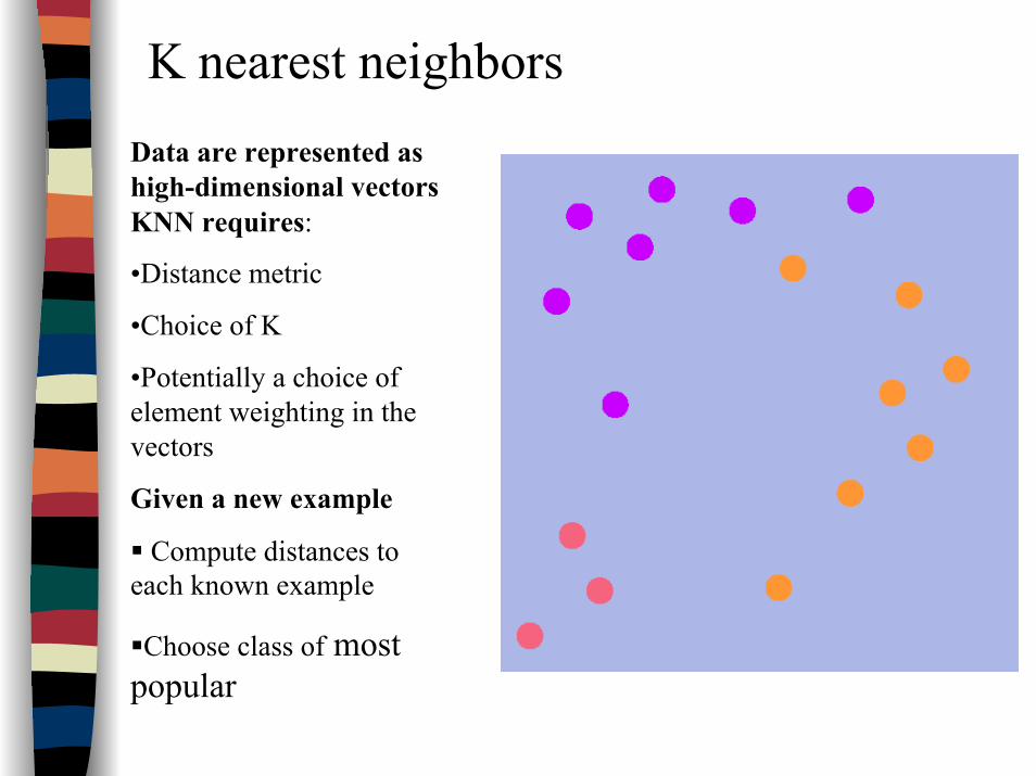
K nearest neighborsData are represented as high-dimensional vectorsKNN requires:
•Distance metric
•Choice of K
•Potentially a choice of element weighting in the vectors
Given a new example
Compute distances to each known example
Choose class of most popular
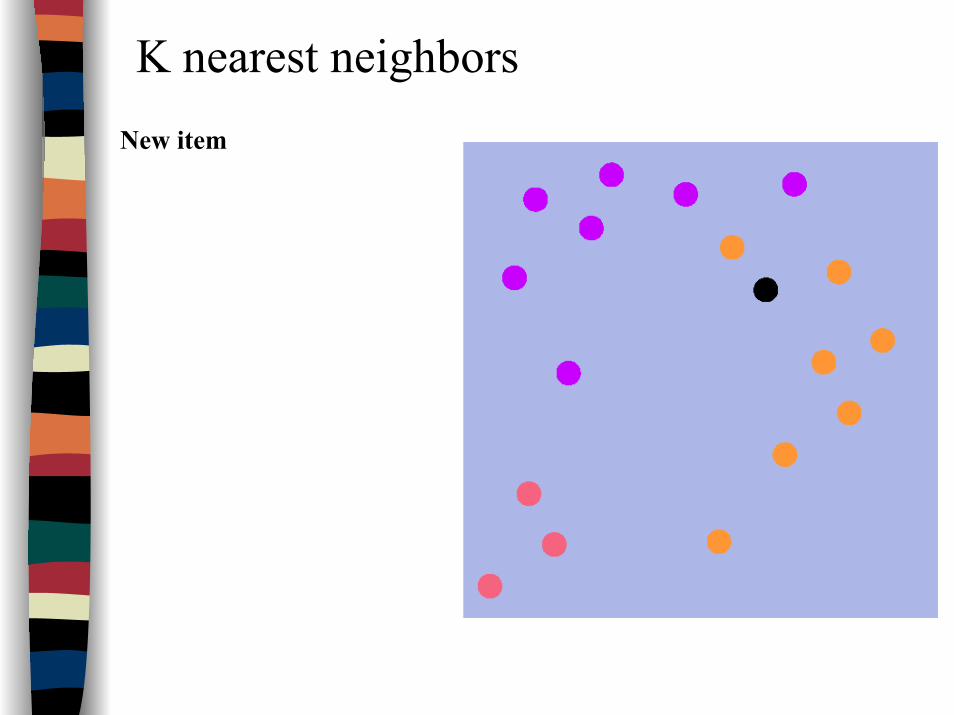
K nearest neighborsNew item
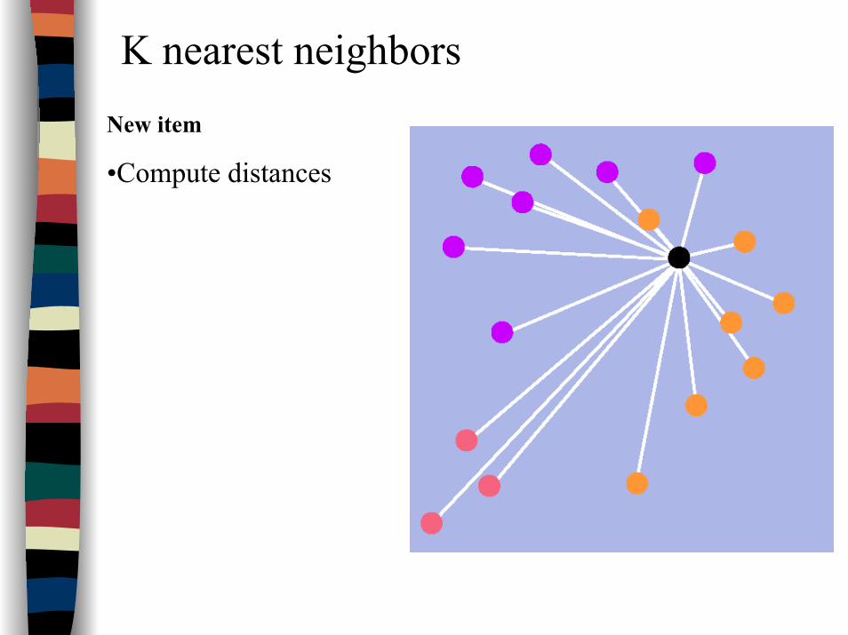
K nearest neighborsNew item
•Compute distances
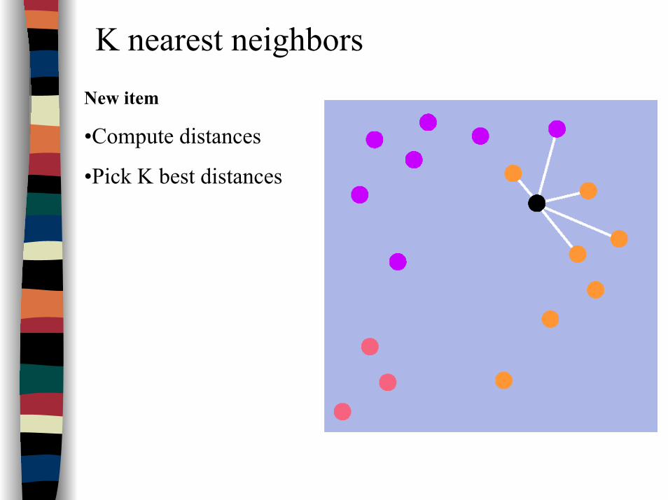
K nearest neighborsNew item
•Compute distances
•Pick K best distances
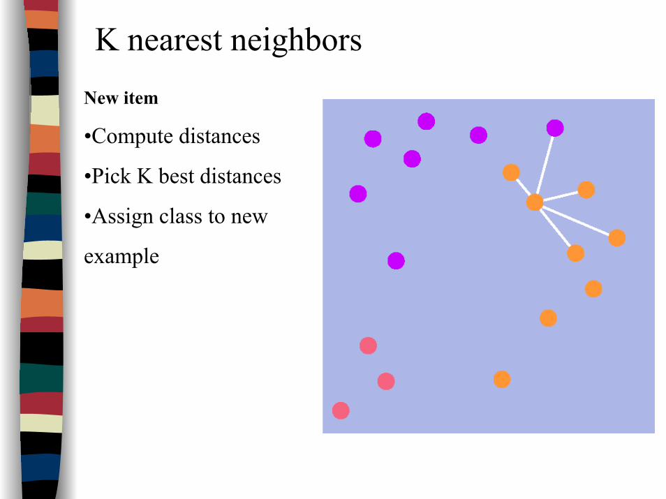
K nearest neighborsNew item
•Compute distances
•Pick K best distances
•Assign class to new
example
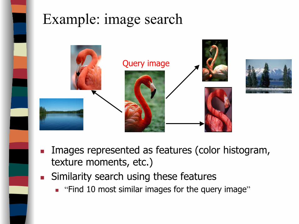
Example: image search
Query image
Images represented as features (color histogram, texture moments, etc.) Similarity search using these features
“Find 10 most similar images for the query image”

Other Applications
Web-page search– “Find 100 most similar pages for a given
page”– Page represented as word-frequency vector– Similarity: vector distance
GIS: “find 5 closest cities of Brisbane”…
Learning Rule 3
Hebbian Learning Rule
D. Hebb
LR3: Hebbian Learning“When an axon of cell A is near enough to excite a cell B and repeatedly or persistently takes place in firing it, some growthprocess or metabolic change takes place in one or both cells such that A’s efficiency, as one of the cells firing B, is increased” (Hebb, 1949)
In other words:
1. If two neurons on either side of a synapse (connection) are activated simultaneously (i.e. synchronously), then the strength of that synapse is selectively increased.
This rule is often supplemented by:
2. If two neurons on either side of a synapse are activated asynchronously, then that synapse is selectively weakened or eliminated. so that chance coincidences do not build up connection strengths.
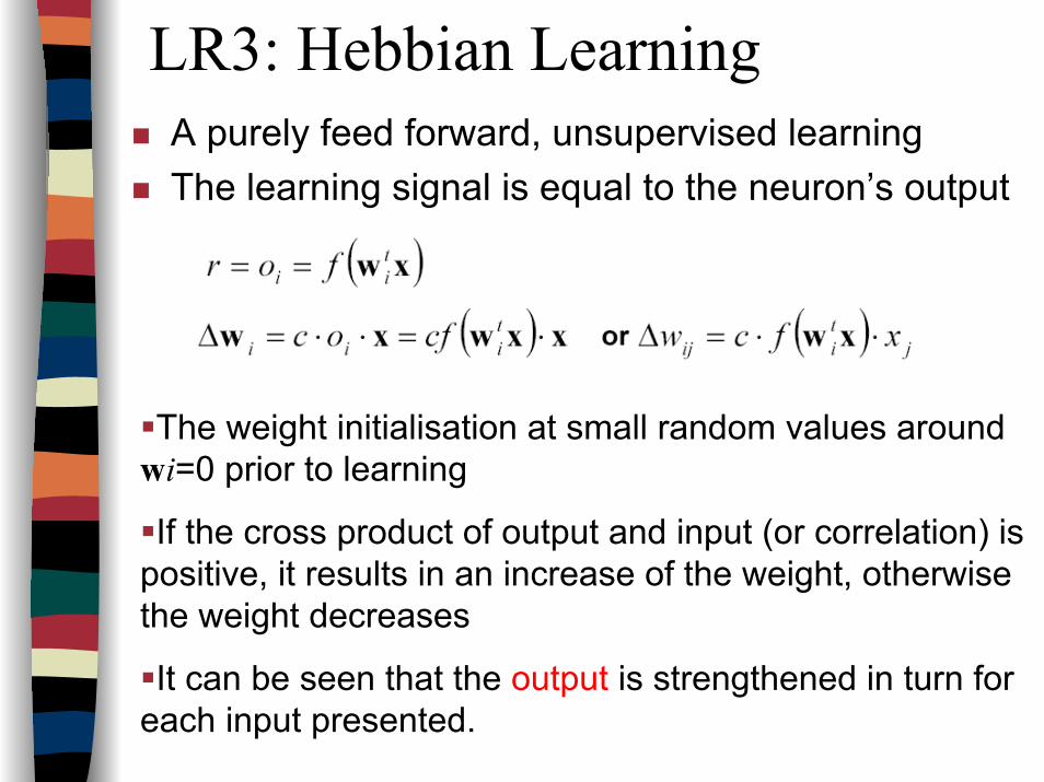
LR3: Hebbian LearningA purely feed forward, unsupervised learning The learning signal is equal to the neuron’s output
The weight initialisation at small random values aroundwi=0 prior to learning
If the cross product of output and input (or correlation) is positive, it results in an increase of the weight, otherwise the weight decreases
It can be seen that the output is strengthened in turn for each input presented.

LR3: Hebbian Learning…Therefore, frequent input patterns will have most influence at the neuron’s weight vector and will eventually produce the largest output.

LR3: Hebbian Learning…In some cases, the Hebbian rule needs to be modified to
counteract unconstrained growth of weight values, which takes place when excitations and responses consistently agree in sign.
This corresponds to the Hebbian learning rule with saturation of the weights at a certain, preset level.
Single Layer Network with Hebb Rule Learning of a set of input-output training vectors is called a HEBB NET
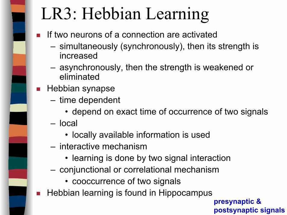
LR3: Hebbian LearningIf two neurons of a connection are activated – simultaneously (synchronously), then its strength is
increased– asynchronously, then the strength is weakened or
eliminatedHebbian synapse– time dependent
• depend on exact time of occurrence of two signals– local
• locally available information is used– interactive mechanism
• learning is done by two signal interaction– conjunctional or correlational mechanism
• cooccurrence of two signalsHebbian learning is found in Hippocampus
presynaptic &postsynaptic signals
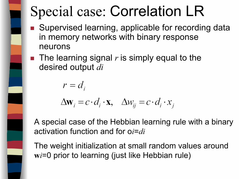
Special case: Correlation LRSupervised learning, applicable for recording data in memory networks with binary response neuronsThe learning signal r is simply equal to the desired output di
A special case of the Hebbian learning rule with a binary activation function and for oi=di
The weight initialization at small random values around wi=0 prior to learning (just like Hebbian rule)

Special case: Correlation LR…
Learning Rule 4
Competitive Learning Rule =Winner-Take-All LR
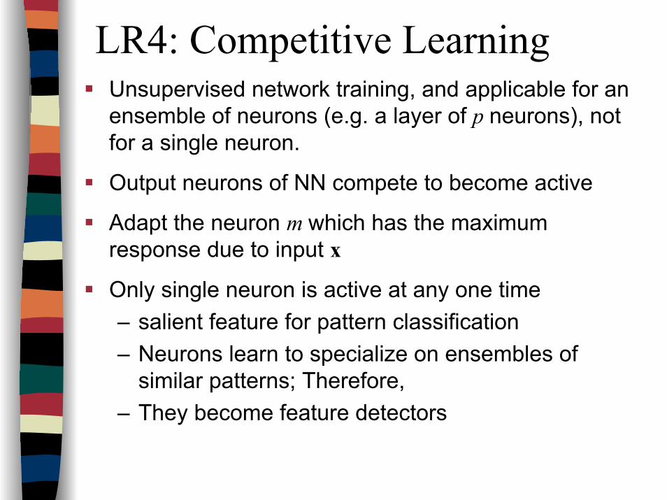
LR4: Competitive LearningUnsupervised network training, and applicable for an ensemble of neurons (e.g. a layer of p neurons), not for a single neuron.
Output neurons of NN compete to become active
Adapt the neuron m which has the maximum response due to input x
Only single neuron is active at any one time– salient feature for pattern classification– Neurons learn to specialize on ensembles of
similar patterns; Therefore,– They become feature detectors
LR4: Competitive Learning…Basic Elements– A set of neurons that are all same except
synaptic weight distribution• respond differently to a given set of input
pattern• A mechanism to compete to respond to
a given input• The winner that wins the competition is
called “winner-takes-all”
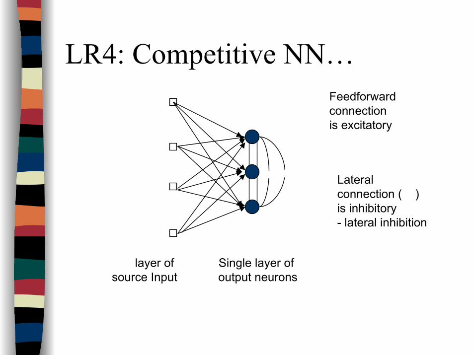
LR4: Competitive NN…Feedforward connectionis excitatory
Lateral connection ( )is inhibitory- lateral inhibition
layer of source Input
Single layer of output neurons
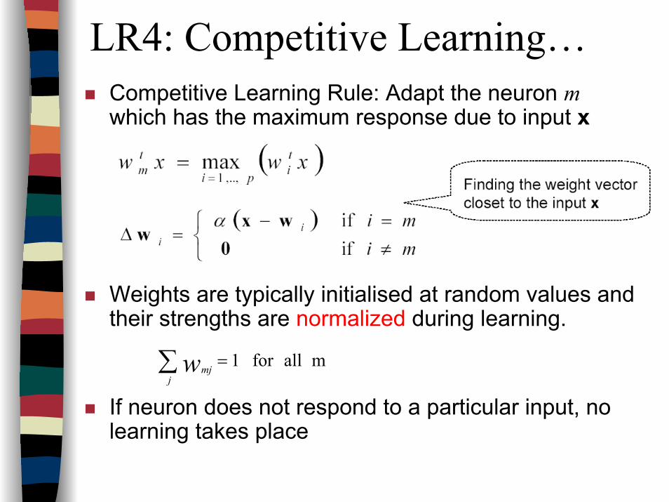
LR4: Competitive Learning…Competitive Learning Rule: Adapt the neuron m which has the maximum response due to input x
Weights are typically initialised at random values and their strengths are normalized during learning.
If neuron does not respond to a particular input, no learning takes place
m allfor 1=∑j
mjw
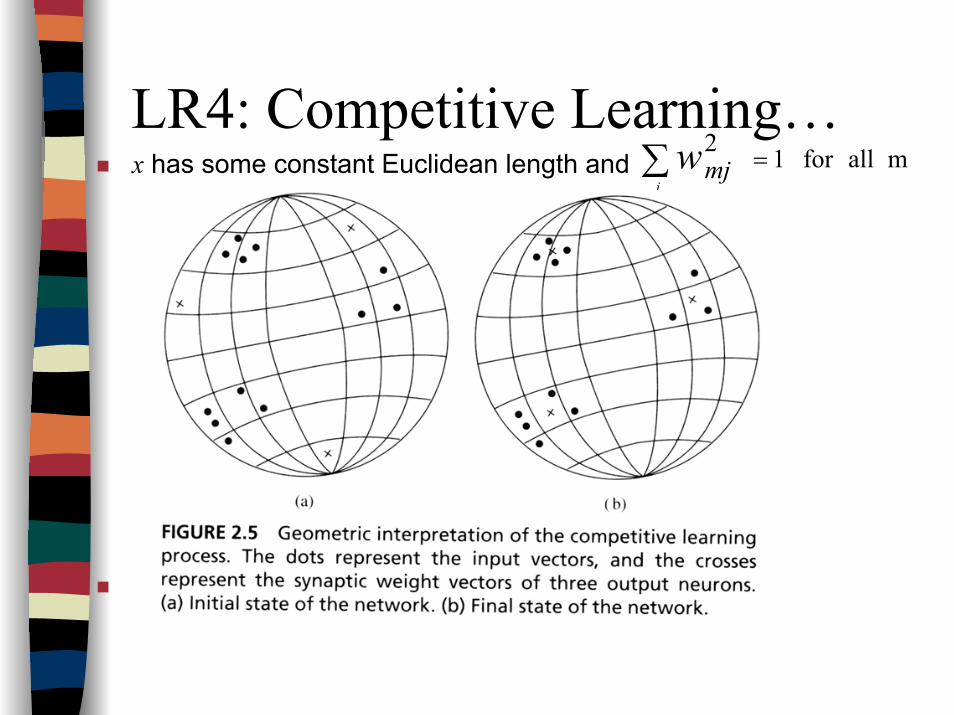
LR4: Competitive Learning…x has some constant Euclidean length and
perform clustering thru competitive learning
m allfor 12=∑
jmjw
LR4: Competitive Learning…What is required for the net to encode the training set is
that the weight vectors become aligned with any clusters present in this set and that each cluster is represented by at least one node. Then, when a vector is presented to the net there will be a node, or group of nodes, which respond maximally to the input and which respond in this way only when this vector is shown at the input
If the net can learn a weight vector configuration like this, without being told explicitly of the existence of clusters at the input, then it is said to undergo a process of self-organised or unsupervised learning. This is to be contrasted with nets which were trained with the delta rule for e.g. where a target vector or output had to be supplied.
LR4: Competitive Learning…In order to achieve this goal, the weight vectors must be
rotated around the sphere so that they line up with the training set. The first thing to notice is that this may be achieved in a
gradual and efficient way by moving the weight vector which is closest (in an angular sense) to the current input vector towards that vector slightly. The node k with the closest vector is that which gives the
greatest input excitation v=w.x since this is just the dot product of the weight and input vectors. As shown below, the weight vector of node k may be aligned more closely with the input if a change is made according to
)(x j mjmj ww −=∆ α
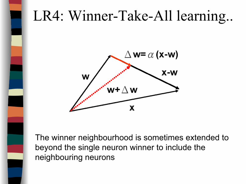
LR4: Winner-Take-All learning..
The winner neighbourhood is sometimes extended to beyond the single neuron winner to include the neighbouring neurons
Learning Rule 5
Boltzman Learning Rule
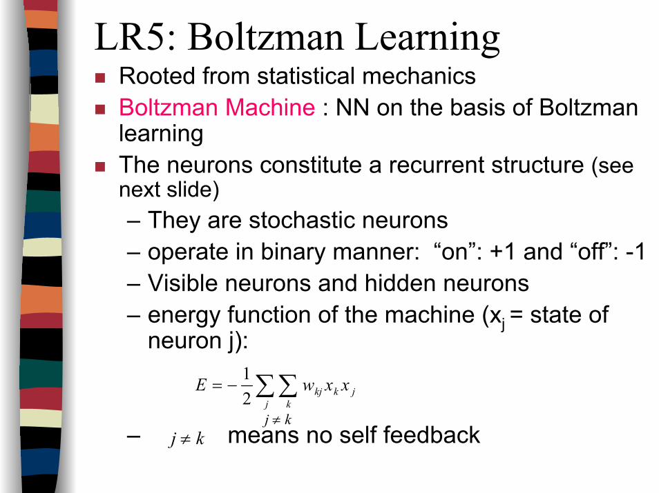
LR5: Boltzman LearningRooted from statistical mechanicsBoltzman Machine : NN on the basis of Boltzman learningThe neurons constitute a recurrent structure (see next slide)– They are stochastic neurons– operate in binary manner: “on”: +1 and “off”: -1– Visible neurons and hidden neurons– energy function of the machine (xj = state of
neuron j):
– means no self feedback
jkj k
kj xxwE ∑ ∑−=21
j ≠ kj ≠ k
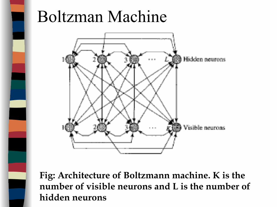
Boltzman Machine
Fig: Architecture of Boltzmann machine. K is the number of visible neurons and L is the number of hidden neurons
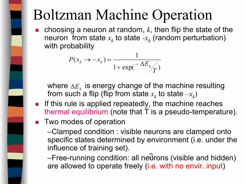
Boltzman Machine Operationchoosing a neuron at random, k, then flip the state of the neuron from state xk to state -xk (random perturbation) with probability
where is energy change of the machine resulting from such a flip (flip from state xk to state –xk)
If this rule is applied repeatedly, the machine reaches thermal equilibrium (note that T is a pseudo-temperature).Two modes of operation–Clamped condition : visible neurons are clamped onto specific states determined by environment (i.e. under the influence of training set).–Free-running condition: all neurons (visible and hidden) are allowed to operate freely (i.e. with no envir. input)
)exp(1
1)(
TExxP
kkk ∆−+
=−→
kE∆
ℑ
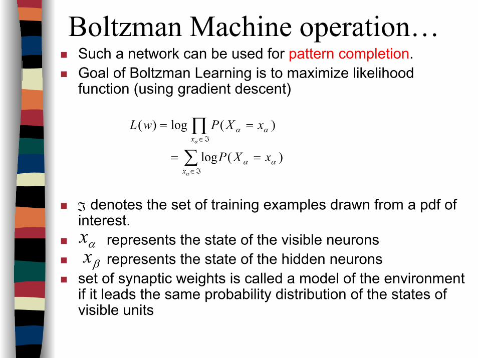
Boltzman Machine operation…Such a network can be used for pattern completion.Goal of Boltzman Learning is to maximize likelihood function (using gradient descent)
denotes the set of training examples drawn from a pdf of interest.
represents the state of the visible neuronsrepresents the state of the hidden neurons
set of synaptic weights is called a model of the environment if it leads the same probability distribution of the states of visible units
ℑ
)(log
)(log)(
αα
αα
α
α
xXP
xXPwL
x
x
==
==
∑
∏
ℑ∈
ℑ∈
αxβx
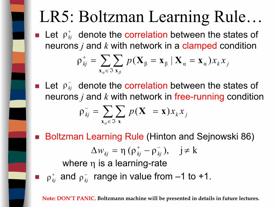
LR5: Boltzman Learning Rule…Let denote the correlation between the states of neurons j and k with network in a clamped condition
Let denote the correlation between the states of neurons j and k with network in free-running condition
Boltzman Learning Rule (Hinton and Sejnowski 86)
where η is a learning-rateand range in value from –1 to +1.
k j ),ρρ( η ≠−=∆ −+kjkjkjw
+kjρ
−kjρ
jkkj xxp )|( ρ ααββ xXxXx x
=== ∑ ∑ℑ∈
+
α β
jkkj xxp )( ρ xXx x
== ∑ ∑ℑ∈
−
α
+kjρ −
kjρ
Note: DON’T PANIC. Boltzmann machine will be presented in details in future lectures.
End of Learning Rules (LR)
Network complexityNo formal methods exist for determining network architecture. For e.g. the number of layers in a feed forward network, the number of nodes in each layer… The next lectures will focus on specific networks.
Suggested Reading.S. Haykin, “Neural Networks”, Prentice-Hall, 1999,
chapter 2, and section 11.7, chapter 11 (for Boltzmannlearning).L. Fausett, “Fundamentals of Neural Networks”,
Prentice-Hall, 1994, Chapter 2, and Section 7.2.2. of chapter 7 (for Boltzmann machine). R.P. Lippmann, “An Introduction to Computing with
Neural Nets”, IEEE Magazine on Acoustics, Signal and Speech Processing, April 1987: 4-22.B. Widrow, “Generalization and Information Storage in
Networks of Adaline “neurons”, Self-Organizing Systems, 1962, ed. MC. Jovitz, G.T. Jacobi, G. Goldstein, Spartan Books, 435-461
References:In addition to the references of the previous slide, the following references were also used to prepare these lecture notes.
1.Berlin Chen Lecture notes: Normal University, Taipei, Taiwan, ROC. http://140.122.185.120
2. Jin Hyung Kim, KAIST Computer Science Dept., CS679 Neural Network lecture notes http://ai.kaist.ac.kr/~jkim/cs679/detail.htm
3. Kevin Gurney lecture notes, “Neural Nets”, Univ. of Sheffield, UK. http://www.shef.ac.uk/psychology/gurney/notes/contents.html
4.Dr John A. Bullinaria, Course Material, Introduction to Neural Networks, http://www.cs.bham.ac.uk/~jxb/inn.html
5.Richard Caruana, lecture notes, Cornell Univ. http://courses.cs.cornell.edu/cs578/2002fa/
6.http://www.free-graphics.com/main.html

References…7. Rothrock-Ling, Wright State Univ. lecture notes:
www.ie.psu.edu/Rothrock/hfe890Spr01/ANN_part1.ppt8. L. Jin, N. Koudas, C. Li, “NNH: Improving Performance of
Nearest-Neighbor Searches Using Histograms”:www.ics.uci.edu/~chenli/pub/NNH.ppt
9. Ajay Jain, UCSF: http://www.cgl.ucsf.edu/Outreach/bmi203/lecture_notes02/lecture7.pdf