Embed Size (px)
Citation preview

© Kavi Arya IIT Bombay 1
CS684 Embedded Systems (Software)
Embedded Applications
Kavi Arya
CSE/ IIT Bombay

© Kavi Arya IIT Bombay 2
Examples of Embedded Systems
We will look at details of • Firebird V robot and simple Digital Camera

© Kavi Arya IIT Bombay 3
Embedded Applications
They are everywhere!
• wristwatches, washing machines, • microwave ovens, • elevators, mobiles, printers • telephone exchanges, • automobiles, aircrafts, …

© Kavi Arya IIT Bombay 4
Common Design Metrics • NRE (Non-recurring engineering) cost • Unit cost • Size (bytes, gates) • Performance (execution time) • Power (more power=> more heat & less battery time) • Flexibility (ability to change functionality) • Time to prototype • Time to market • Maintainability • Correctness • Safety (probability that system won’t cause harm)

© Kavi Arya IIT Bombay 5
Embedded Apps
• A modern home – Has a few general purpose PCs/laptops – but has a dozen of embedded systems.
• More prevalent in industrial sectors – 10’s of embedded computers in modern
automobiles – chemical and nuclear power plants

© Kavi Arya IIT Bombay 6
Embedded Applications An embedded system typically has a digital signal processor and a variety of I/O devices connected to sensors and actuators.
Computer (controller) is surrounded by other subsystems, sensors and actuators
Computer -- Controller's function is : • To monitor parameters of physical processes of its surrounding system • To control these processes whenever needed.
© Kavi Arya IIT Bombay 7
Simple Examples A simple thermostat controller • periodically reads temperature of chamber • switches on or off the cooling system. A pacemaker • constantly monitors the heart • paces the heart when heart beats are missed

© Kavi Arya IIT Bombay 8
1. Digital Camera: An Embedded System Source: Embedded System Design: Frank Vahid/ Tony Givargis
(John Wiley & Sons, Inc.2014)
• Introduction to a simple digital camera
• Requirements specification • Designer’s perspective
• Design exploration

© Kavi Arya IIT Bombay 9
Requirements Specification • System’s reqmts – what system should do
– Nonfunctional requirements • Constraints on design metrics
(e.g., “should use 0.001 watt or less”) – Functional requirements
• System’s behavior (e.g., “output X to be input Y times 2”)
– ….
© Kavi Arya IIT Bombay 10
Requirements Specification…
Initial specification may be very general and come from marketing dept.
• E.g., short document detailing market need for a low-end digital camera that: – Captures/ stores at least 50 low-res images and uploads to PC, – Costs around $100 with single medium-size IC costing < $25, – Has long as possible battery life, – Has expected sales volume of 200,000 if market entry < 6 months, – 100,000 if between 6 and 12 months, – Insignificant sales beyond 12 months

© Kavi Arya IIT Bombay 11
Nonfunctional requirements
• Design metrics of importance based on initial specification – Performance: time required to process image – Size: number of elementary logic gates (2-input
NAND gate) in IC – Power: measure of avg. electrical energy
consumed while processing – Energy: battery lifetime (power x time)
© Kavi Arya IIT Bombay 12
Nonfunctional requirements…
• Constrained metrics – Values must be below (sometimes above)
certain threshold • Optimization metrics
– Improve as much as possible to improve product • Metric can be both constrained and
optimization
© Kavi Arya IIT Bombay 13
Nonfunctional requirements…
• Power – Must operate below certain temperature
(cooling fan not possible) – Therefore, constrained metric
• Energy – Reducing power or time reduces energy – Optimized metric: want battery to last as long
as possible
© Kavi Arya IIT Bombay 14
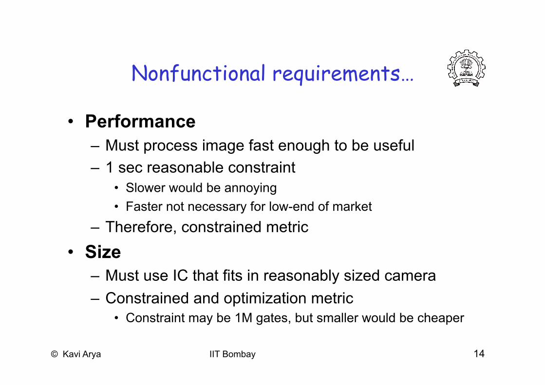
Nonfunctional requirements…
• Performance – Must process image fast enough to be useful – 1 sec reasonable constraint
• Slower would be annoying • Faster not necessary for low-end of market
– Therefore, constrained metric
• Size – Must use IC that fits in reasonably sized camera – Constrained and optimization metric
• Constraint may be 1M gates, but smaller would be cheaper

© Kavi Arya IIT Bombay 15
Example: Panasonic Lumix DMC TZ5
• 9.1 effective Megapixels • 28-280mm equiv lens, 10x optical zoom & 4x Digital Zoom • 3.0-inch LCD with 460,000 dots resolution • Optical Image Stabilizer • ISO sensitivity up to 6400 • Face Detection AF • 6 shooting modes, 23 scene modes inc. Intelligent Auto mode • Venus Engine IV processor • HD output • In-Camera Editing
$300

© Kavi Arya IIT Bombay 16
1. Digital Camera: An Embedded System
Design – Four implementations – Issues:
• General-purpose vs. single-purpose processors?
• Partitioning of functionality among different processor types?

© Kavi Arya IIT Bombay 17
Functional Design & Mapping
HW1 HW2 HW3 HW4Hardware Interface
RTOS/Drivers
Thre
adArchitectural Design
F1F2
F3F4
F5Functional
Design
(F3) (F4)
(F5)
(F2)

© Kavi Arya IIT Bombay 18
Introduction to a simple digital camera • Captures images • Stores images in digital format
– No film – Multiple images stored in camera
• Number depends on memory and bits/image
• Downloads images to PC – Serial comm (USB, etc.) – Wireless (Bluetooth, 802.11, …)

© Kavi Arya IIT Bombay 19
Introduction to a simple digital camera…
• Only possible in couple of decades – Systems-on-a-chip
• Multiple processors and memories on one IC – High-capacity flash memory
• Very simple description used for example – Many more features with real digital camera
• Variable size images, image deletion, digital stretching, zooming in and out, etc.

© Kavi Arya IIT Bombay 20
Designer’s perspective
• Two key tasks 1. Processing images and storing in memory
• When shutter pressed: – Image captured – Converted to digital form by charge-coupled device
(CCD) – Compressed and archived in internal memory
2. Uploading images to PC • Digital camera attached to PC • Software to transmit archived images serially

© Kavi Arya IIT Bombay 21
Charge-coupled device (CCD) • Special sensor that captures an image • Light-sensitive silicon solid-state device composed of
many cells
Light ⇒ charge ⇒ 8-bit value 0 => no exposure 255=> intense light
Some columns covered with black strip. Light-intensity here used for zero-bias adjustment
Electromechanical shutter activates to expose cells to light
Circuitry discharges cells, activates shutter, reads 8-bit value of each cell.
Values clocked out of CCD by external logic through std parallel bus interface.
Lens area
Pixel columns
Covered columns
Electronic circuitry
Electro-mechanical
shutter
Pixe
l row
s

© Kavi Arya IIT Bombay 22
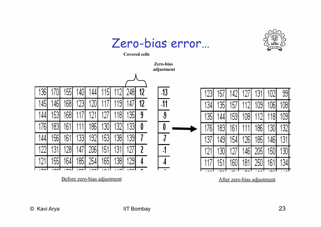
Zero-bias error • Manufacturing errors cause cells to measure
slightly above or below actual light intensity • Error typically same across columns, but different
across rows • Some of left most columns blocked by black paint
to detect zero-bias error – Reading of non-zero in blocked cells is zero-bias error – Each row corrected by subtracting avg error in blocked cells
for that row
© Kavi Arya IIT Bombay 23
Zero-bias error… Covered cells
Before zero-bias adjustment After zero-bias adjustment
Zero-bias adjustment

© Kavi Arya IIT Bombay 24
Compression • Store more images • Transmit image to PC in less time • JPEG (Joint Photographic Experts Group)

© Kavi Arya IIT Bombay 25
Compression…
JPEG (Joint Photographic Experts Group) – Popular standard format for representing digital images
in a compressed form – Provides for a number of different modes of operation – Sequential Mode used here provides high compression
ratios using DCT (Discrete Cosine Transform) (others are -- progressive, lossless, hierarchical)
– Image data divided into blocks of 8 x 8 pixels – 3 steps performed on each block DCT, Quantization, Huffman encoding

© Kavi Arya IIT Bombay 26
DCT step • Transforms original 8 x 8 block into a
cosine-frequency domain – Upper-left corner values represent more of
essence of image (Average for the image) – Lower-right corner values represent finer
details • Can reduce precision of these values and
retain reasonable image quality • Quantize – many may become 0
© Kavi Arya IIT Bombay 27
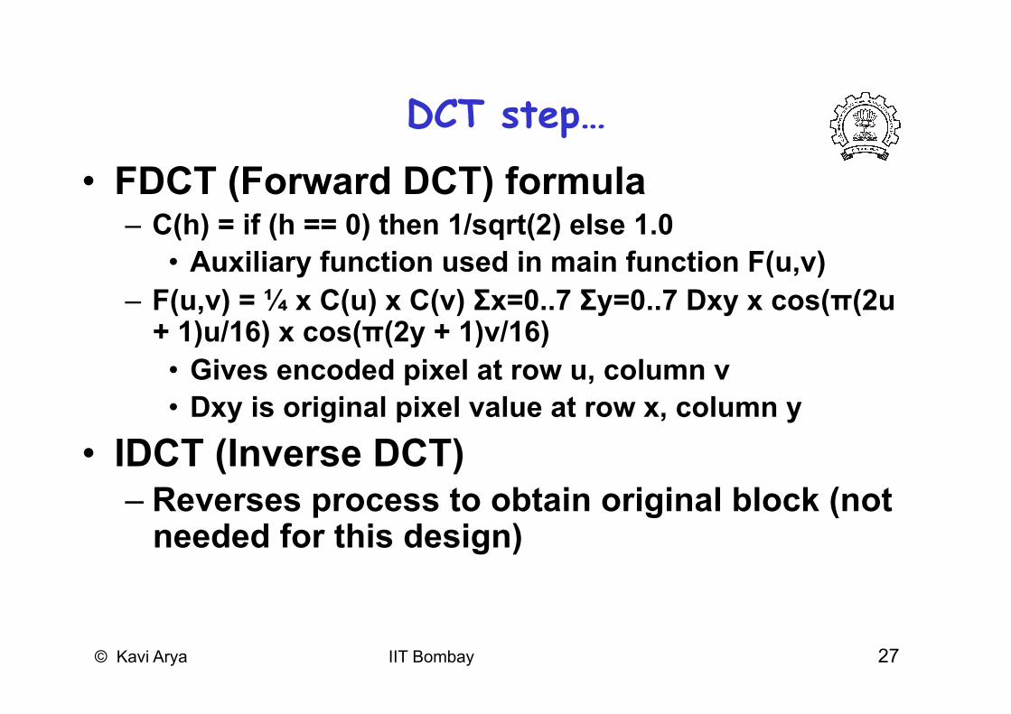
DCT step… • FDCT (Forward DCT) formula
– C(h) = if (h == 0) then 1/sqrt(2) else 1.0 • Auxiliary function used in main function F(u,v)
– F(u,v) = ¼ x C(u) x C(v) Σx=0..7 Σy=0..7 Dxy x cos(π(2u + 1)u/16) x cos(π(2y + 1)v/16) • Gives encoded pixel at row u, column v • Dxy is original pixel value at row x, column y
• IDCT (Inverse DCT) – Reverses process to obtain original block (not
needed for this design)

© Kavi Arya IIT Bombay 28
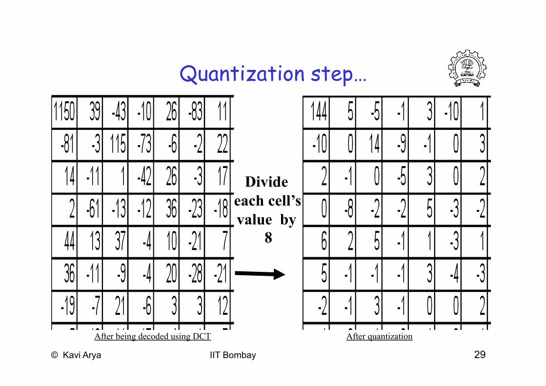
Quantization step
• Achieve high compression ratio by reducing image quality – Reduce bit precision of encoded data
• Fewer bits needed for encoding • One way is divide all values by factor of 2
– Simple right shifts can do this – General: table driven mapping
– Dequantization reverses process for decompression
© Kavi Arya IIT Bombay 29
Quantization step…
After being decoded using DCT After quantization
Divide each cell’s value by
8

© Kavi Arya IIT Bombay 30
• Serialize 8 x 8 block of pixels – Values are converted into single list using zigzag pattern
Huffman encoding step
Usually, first item of blocks are stored differentially Zigzag brings equal values together => run-length encoding

© Kavi Arya IIT Bombay 31
• Perform Huffman encoding – More frequently occurring pixels assigned
short binary code – Longer binary codes left for less
frequently occurring pixels • Each pixel in serial list converted to
Huffman encoded values – Much shorter list, thus compression
Huffman encoding step…
© Kavi Arya IIT Bombay 32
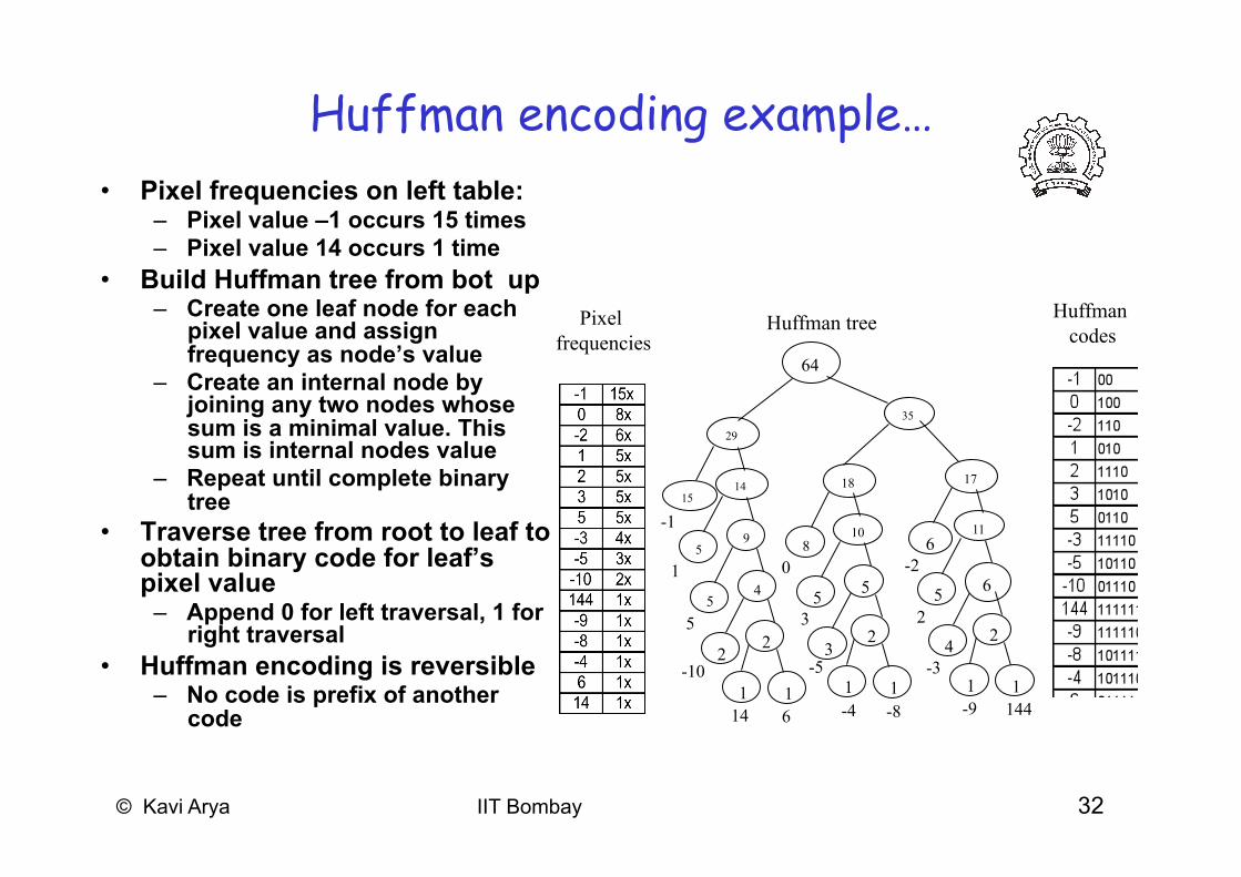
Huffman encoding example… • Pixel frequencies on left table:
– Pixel value –1 occurs 15 times – Pixel value 14 occurs 1 time
• Build Huffman tree from bot up – Create one leaf node for each
pixel value and assign frequency as node’s value
– Create an internal node by joining any two nodes whose sum is a minimal value. This sum is internal nodes value
– Repeat until complete binary tree
• Traverse tree from root to leaf to obtain binary code for leaf’s pixel value
– Append 0 for left traversal, 1 for right traversal
• Huffman encoding is reversible – No code is prefix of another
code 144
5 3 2
1 0 -2
-1
-10 -5 -3
-4 -8 -9 6 14 1 1
2
1 1
2
1
22
4
3
5
4
6 5
9
5
10
5
11 5
14
6
17
8
18 15
29
35
64
1
Pixel frequencies
Huffman tree Huffman codes

© Kavi Arya IIT Bombay 33
Archive step • Record starting address and image size
– Can use linked list • One possible way to archive images
– If max number of images archived is N: • Set aside memory for N addresses and N image-size variables • Keep counter for location of next available address • Initialize addresses and image-size variables to 0 • Set global memory address to N x 4
– Assuming addresses, image-size variables occupy N x 4 bytes • First image archived starting at address N x 4 • Global memory address updated to N x 4 + (compressed image
size) • Memory requirement based on N, image size, and average
compression ratio

© Kavi Arya IIT Bombay 34
Uploading to PC
• When connected to PC and upload command received – Read images from memory – Transmit serially using UART* – While transmitting
• Reset pointers, image-size variables and global memory pointer accordingly
*UART (Universal Asynchronous Receiver Transmitter)
© Kavi Arya IIT Bombay 35
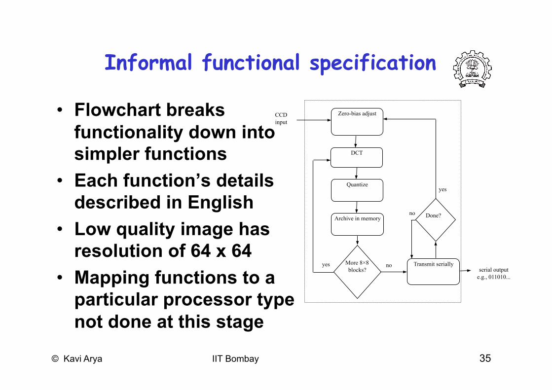
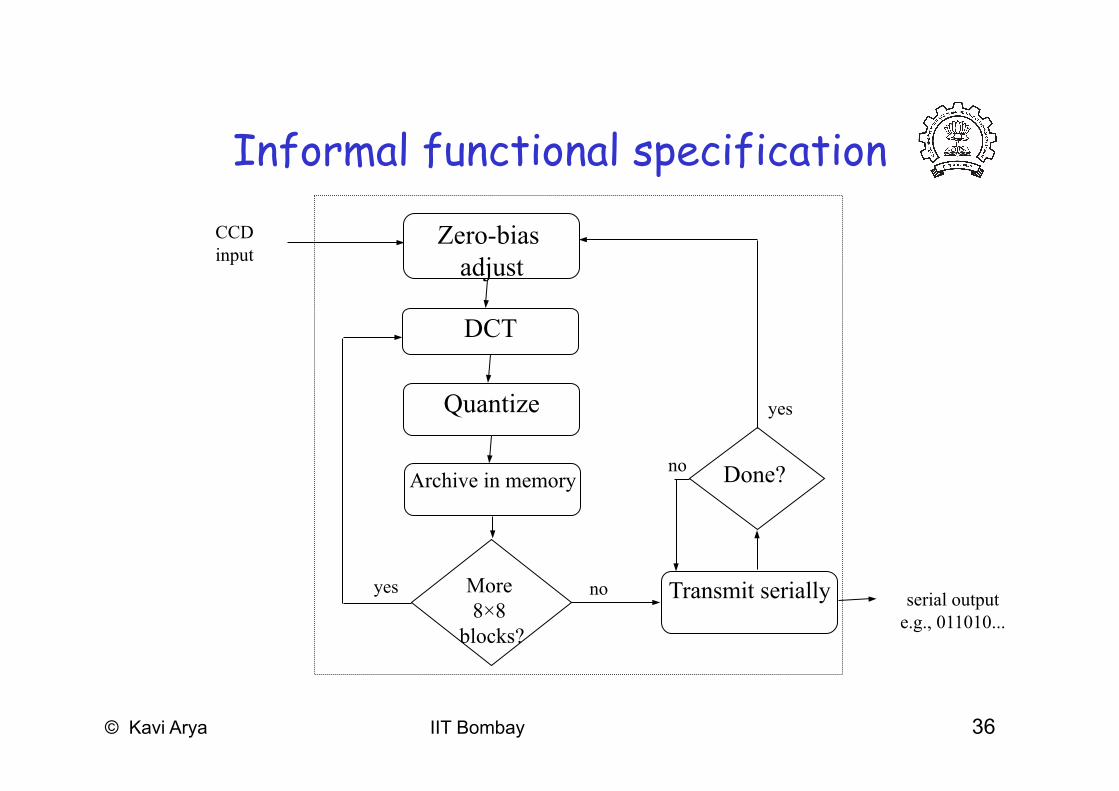
Informal functional specification
• Flowchart breaks functionality down into simpler functions
• Each function’s details described in English
• Low quality image has resolution of 64 x 64
• Mapping functions to a particular processor type not done at this stage
serial output e.g., 011010...
yes no
CCD input
Zero-bias adjust
DCT
Quantize
Archive in memory
More 8×8 blocks?
Transmit serially
yes
no Done?
© Kavi Arya IIT Bombay 36
Informal functional specification
serial output e.g., 011010...
yes no
CCD input
Zero-bias adjust
DCT
Quantize
Archive in memory
More 8×8
blocks?
Transmit serially
yes
no Done?
© Kavi Arya IIT Bombay 37
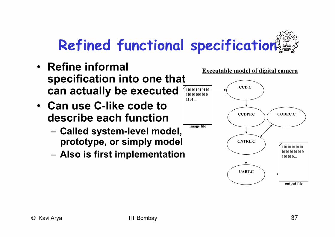
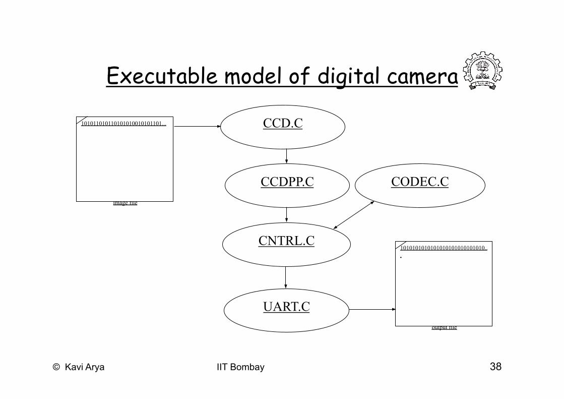
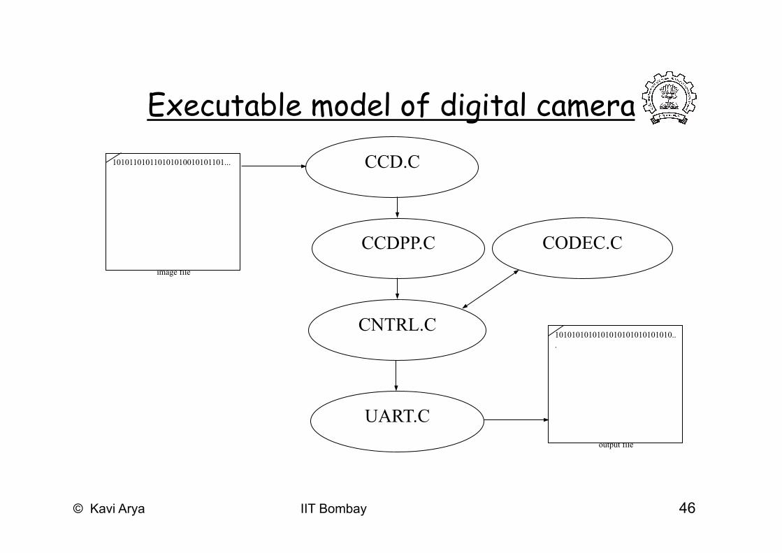
Refined functional specification • Refine informal
specification into one that can actually be executed
• Can use C-like code to describe each function – Called system-level model,
prototype, or simply model – Also is first implementation
image file
101011010110101010010101101...
CCD.C
CNTRL.C
UART.C
output file
1010101010101010101010101010...
CODEC.C CCDPP.C
Executable model of digital camera
© Kavi Arya IIT Bombay 38
Executable model of digital camera
image file
101011010110101010010101101... CCD.C
CNTRL.C
UART.C output file
1010101010101010101010101010...
CODEC.C CCDPP.C

© Kavi Arya IIT Bombay 39
Refined functional specification…
• Provides insight into operations of system – Profiling finds computationally intensive functions
• Can obtain sample output used to verify correctness of final implementation
© Kavi Arya IIT Bombay 40
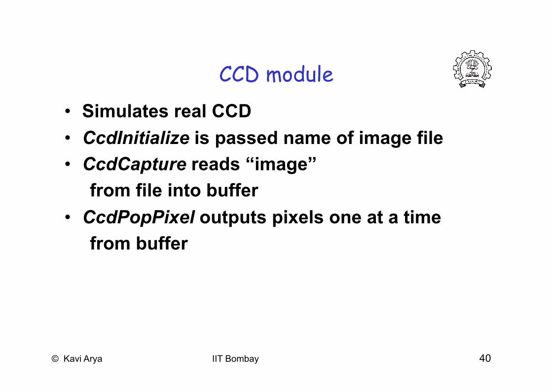
CCD module • Simulates real CCD • CcdInitialize is passed name of image file • CcdCapture reads “image” from file into buffer • CcdPopPixel outputs pixels one at a time from buffer

© Kavi Arya IIT Bombay 41
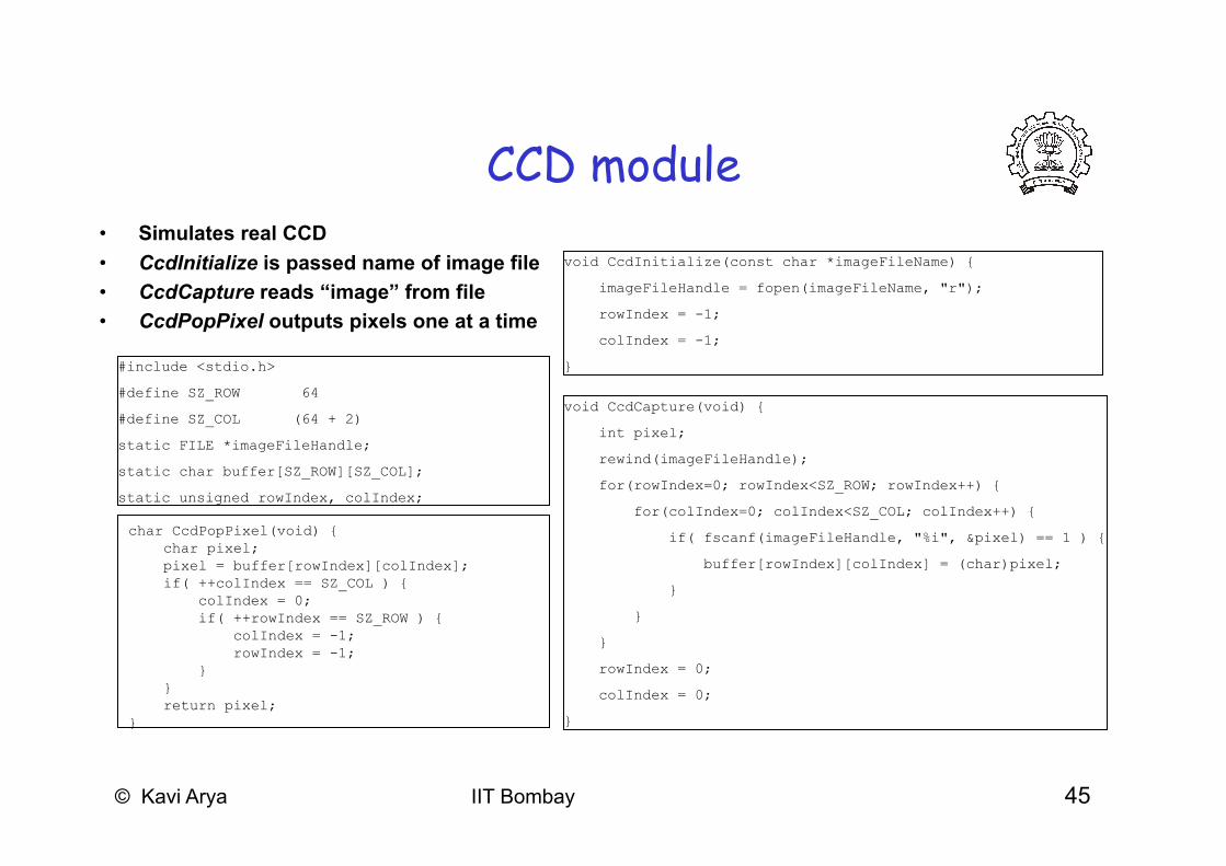
CCD module • Simulates real CCD • CcdInitialize is passed name of image file • CcdCapture reads “image” from file • CcdPopPixel outputs pixels one at a time
#include <stdio.h>
#define SZ_ROW 64
#define SZ_COL (64 + 2)
static FILE *imageFileHandle;
static char buffer[SZ_ROW][SZ_COL];
static unsigned rowIndex, colIndex;
© Kavi Arya IIT Bombay 42
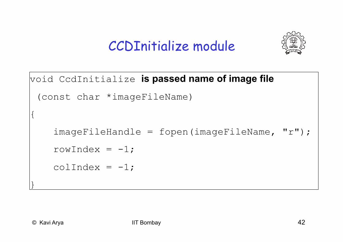
CCDInitialize module
void CcdInitialize is passed name of image file
(const char *imageFileName)
{
imageFileHandle = fopen(imageFileName, "r");
rowIndex = -1;
colIndex = -1;
}

© Kavi Arya IIT Bombay 43
CCDCapture module void CcdCapture(void) {reads “image” from file into buffer int pixel;
rewind(imageFileHandle);
for(rowIndex=0; rowIndex<SZ_ROW; rowIndex++) {
for(colIndex=0; colIndex<SZ_COL; colIndex++) {
if( fscanf(imageFileHandle, "%i", &pixel) == 1 ) {
buffer[rowIndex][colIndex] = (char)pixel;
}
}
} rowIndex = 0; colIndex = 0;
}

© Kavi Arya IIT Bombay 44
CCDPopPixel module • CcdPopPixel outputs pixels one at a time from buffer
char CcdPopPixel(void) { char pixel; pixel = buffer[rowIndex][colIndex]; if( ++colIndex == SZ_COL ) { colIndex = 0; if( ++rowIndex == SZ_ROW ) { colIndex = -1; rowIndex = -1; } } return pixel; }
© Kavi Arya IIT Bombay 45
CCD module • Simulates real CCD • CcdInitialize is passed name of image file • CcdCapture reads “image” from file • CcdPopPixel outputs pixels one at a time
char CcdPopPixel(void) { char pixel; pixel = buffer[rowIndex][colIndex]; if( ++colIndex == SZ_COL ) { colIndex = 0; if( ++rowIndex == SZ_ROW ) { colIndex = -1; rowIndex = -1; } } return pixel; }
#include <stdio.h>
#define SZ_ROW 64
#define SZ_COL (64 + 2)
static FILE *imageFileHandle;
static char buffer[SZ_ROW][SZ_COL];
static unsigned rowIndex, colIndex;
void CcdInitialize(const char *imageFileName) {
imageFileHandle = fopen(imageFileName, "r");
rowIndex = -1;
colIndex = -1;
}
void CcdCapture(void) {
int pixel;
rewind(imageFileHandle);
for(rowIndex=0; rowIndex<SZ_ROW; rowIndex++) {
for(colIndex=0; colIndex<SZ_COL; colIndex++) {
if( fscanf(imageFileHandle, "%i", &pixel) == 1 ) {
buffer[rowIndex][colIndex] = (char)pixel;
}
}
}
rowIndex = 0;
colIndex = 0;
}
© Kavi Arya IIT Bombay 46
Executable model of digital camera
image file
101011010110101010010101101... CCD.C
CNTRL.C
UART.C output file
1010101010101010101010101010...
CODEC.C CCDPP.C

© Kavi Arya IIT Bombay 47
CCDPP (CCD PreProcessing) module • Performs zero-bias adjustment • CcdppCapture uses CcdCapture and CcdPopPixel to obtain image • Performs zero-bias adjustment after each row read in

© Kavi Arya IIT Bombay 48
CCDPP (CCD PreProcessing) module • Performs zero-bias adjustment • CcdppCapture uses CcdCapture and CcdPopPixel to
obtain image • Performs zero-bias adjustment after each row read in
#define SZ_ROW 64
#define SZ_COL 64
static char buffer[SZ_ROW][SZ_COL];
static unsigned rowIndex, colIndex;
void CcdppInitialize() {
rowIndex = -1;
colIndex = -1;
}
void CcdppCapture(void) {
char bias;
CcdCapture();
for(rowIndex=0; rowIndex<SZ_ROW; rowIndex++) {
for(colIndex=0; colIndex<SZ_COL; colIndex++) {
buffer[rowIndex][colIndex] = CcdPopPixel();
}
bias = (CcdPopPixel() + CcdPopPixel()) / 2;
for(colIndex=0; colIndex<SZ_COL; colIndex++) {
buffer[rowIndex][colIndex] -= bias;
}
}
rowIndex = 0;
colIndex = 0;
}
char CcdppPopPixel(void) {
char pixel;
pixel = buffer[rowIndex][colIndex];
if( ++colIndex == SZ_COL ) {
colIndex = 0;
if( ++rowIndex == SZ_ROW ) {
colIndex = -1;
rowIndex = -1;
}
}
return pixel;
}

© Kavi Arya IIT Bombay 49
CCDPPCapture module void CcdppCapture(void) {
char bias;
CcdCapture();
for(rowIndex=0; rowIndex<SZ_ROW; rowIndex++) {
for(colIndex=0; colIndex<SZ_COL; colIndex++) {
buffer[rowIndex][colIndex] = CcdPopPixel();
}
bias = (CcdPopPixel() + CcdPopPixel()) / 2;
for(colIndex=0; colIndex<SZ_COL; colIndex++) {
buffer[rowIndex][colIndex] -= bias;
}
} rowIndex = 0; colIndex = 0; }

© Kavi Arya IIT Bombay 50
Executable model of digital camera
image file
101011010110101010010101101... CCD.C
CNTRL.C
UART.C output file
1010101010101010101010101010...
CODEC.C CCDPP.C
© Kavi Arya IIT Bombay 51
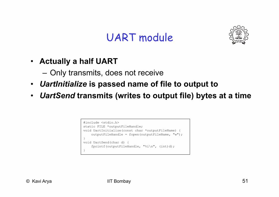
UART module
• Actually a half UART – Only transmits, does not receive
• UartInitialize is passed name of file to output to • UartSend transmits (writes to output file) bytes at a time
#include <stdio.h> static FILE *outputFileHandle; void UartInitialize(const char *outputFileName) { outputFileHandle = fopen(outputFileName, "w"); } void UartSend(char d) { fprintf(outputFileHandle, "%i\n", (int)d); }

© Kavi Arya IIT Bombay 52
Executable model of digital camera
image file
101011010110101010010101101... CCD.C
CNTRL.C
UART.C output file
1010101010101010101010101010...
CODEC.C CCDPP.C

© Kavi Arya IIT Bombay 53
CODEC module • Models FDCT* encoding • ibuffer holds original 8 x 8 block • obuffer holds encoded 8 x 8 block • CodecPushPixel called 64x to fill ibuffer w/original block • CodecDoFdct called once to transform 8 x 8 block
– Explained in next slide • CodecPopPixel called 64 times to retrieve encoded block
from obuffer
*Forward Discrete Cosine Transform

© Kavi Arya IIT Bombay 54
CODEC module • Models FDCT encoding • ibuffer holds original 8 x 8 block • obuffer holds encoded 8 x 8
block • CodecPushPixel called 64 times
to fill ibuffer with original block • CodecDoFdct called once to
transform 8 x 8 block – Explained in next slide
• CodecPopPixel called 64 times to retrieve encoded block from obuffer
static short ibuffer[8][8], obuffer[8][8], idx;
void CodecInitialize(void) { idx = 0; }
void CodecDoFdct(void) {
int x, y;
for(x=0; x<8; x++) {
for(y=0; y<8; y++)
obuffer[x][y] = FDCT(x, y, ibuffer);
}
idx = 0;
}
void CodecPushPixel(short p) {
if( idx == 64 ) idx = 0;
ibuffer[idx / 8][idx % 8] = p; idx++;
}
short CodecPopPixel(void) {
short p;
if( idx == 64 ) idx = 0;
p = obuffer[idx / 8][idx % 8]; idx++;
return p;
}

© Kavi Arya IIT Bombay 55
FDCT (Forward DCT) formula
C(h) = if (h == 0) then 1/sqrt(2) else 1.0 • Auxiliary function used in main function F(u,v)
F(u,v) = ¼ x C(u) x C(v) Σx=0..7 Σy=0..7 Dxy x cos(π(2x + 1)u/16) x cos(π(2y + 1)v/16) = ¼ x C(u) x C(v) Σx=0..7 cos(π(2x + 1)u/16) x Σy=0..7 Dxy x cos(π(2y + 1)v/16)
• Gives encoded pixel at row u, column v • Dxy is original pixel value at row x, column y

© Kavi Arya IIT Bombay 56
CODEC… • Implementing FDCT formula • Only 64 possible inputs to COS, so table can be
used to save performance time – Floating-point values multiplied by 32,678 and rounded
to nearest integer – 32,678 chosen to store each value in 2 bytes of memory – Fixed-point representation explained more later
• FDCT unrolls inner loop of summation, implements outer summation as two consecutive for loops

© Kavi Arya IIT Bombay 57
CODEC… • Implementing FDCT formula • Only 64 possible inputs to COS, so
table can be used to save performance time
– Floating-point values multiplied by 32,678 and rounded to nearest integer
– 32,678 chosen in order to store each value in 2 bytes of memory
– Fixed-point representation explained more later
• FDCT unrolls inner loop of summation, implements outer summation as two consecutive for loops
static const short COS_TABLE[8][8] = {
{ 32768, 32138, 30273, 27245, 23170, 18204, 12539, 6392 },
{ 32768, 27245, 12539, -6392, -23170, -32138, -30273, -18204 },
{ 32768, 18204, -12539, -32138, -23170, 6392, 30273, 27245 },
{ 32768, 6392, -30273, -18204, 23170, 27245, -12539, -32138 },
{ 32768, -6392, -30273, 18204, 23170, -27245, -12539, 32138 },
{ 32768, -18204, -12539, 32138, -23170, -6392, 30273, -27245 },
{ 32768, -27245, 12539, 6392, -23170, 32138, -30273, 18204 },
{ 32768, -32138, 30273, -27245, 23170, -18204, 12539, -6392 }
};
static int FDCT(int u, int v, short img[8][8]) {
double s[8], r = 0; int x;
for(x=0; x<8; x++) {
s[x] = img[x][0] * COS(0, v) + img[x][1] * COS(1, v) +
img[x][2] * COS(2, v) + img[x][3] * COS(3, v) +
img[x][4] * COS(4, v) + img[x][5] * COS(5, v) +
img[x][6] * COS(6, v) + img[x][7] * COS(7, v);
}
for(x=0; x<8; x++) r += s[x] * COS(x, u);
return (short)(r * .25 * C(u) * C(v));
}
static short ONE_OVER_SQRT_TWO = 23170;
static double COS(int xy, int uv) {
return COS_TABLE[xy][uv] / 32768.0;
}
static double C(int h) {
return h ? 1.0 : ONE_OVER_SQRT_TWO / 32768.0;
}

© Kavi Arya IIT Bombay 58
Executable model of digital camera
image file
101011010110101010010101101... CCD.C
CNTRL.C
UART.C output file
1010101010101010101010101010...
CODEC.C CCDPP.C

© Kavi Arya IIT Bombay 59
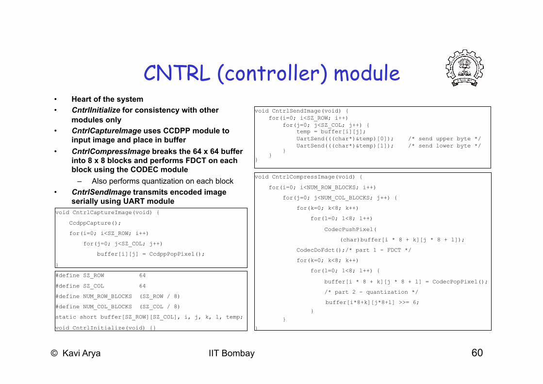
CNTRL (controller) module • Heart of the system • CntrlCaptureImage uses CCDPP module to input image
and place in buffer • CntrlCompressImage breaks the 64 x 64 buffer into 8 x 8
blocks and performs FDCT on each block using the CODEC module – Also performs quantization on each block
• CntrlSendImage transmits encoded image serially using UART module
© Kavi Arya IIT Bombay 60
CNTRL (controller) module • Heart of the system • CntrlInitialize for consistency with other
modules only • CntrlCaptureImage uses CCDPP module to
input image and place in buffer • CntrlCompressImage breaks the 64 x 64 buffer
into 8 x 8 blocks and performs FDCT on each block using the CODEC module
– Also performs quantization on each block • CntrlSendImage transmits encoded image
serially using UART module
void CntrlSendImage(void) { for(i=0; i<SZ_ROW; i++) for(j=0; j<SZ_COL; j++) { temp = buffer[i][j]; UartSend(((char*)&temp)[0]); /* send upper byte */ UartSend(((char*)&temp)[1]); /* send lower byte */ } } }
#define SZ_ROW 64
#define SZ_COL 64
#define NUM_ROW_BLOCKS (SZ_ROW / 8)
#define NUM_COL_BLOCKS (SZ_COL / 8)
static short buffer[SZ_ROW][SZ_COL], i, j, k, l, temp;
void CntrlInitialize(void) {}
void CntrlCaptureImage(void) {
CcdppCapture();
for(i=0; i<SZ_ROW; i++)
for(j=0; j<SZ_COL; j++)
buffer[i][j] = CcdppPopPixel();
}
void CntrlCompressImage(void) {
for(i=0; i<NUM_ROW_BLOCKS; i++)
for(j=0; j<NUM_COL_BLOCKS; j++) {
for(k=0; k<8; k++)
for(l=0; l<8; l++)
CodecPushPixel(
(char)buffer[i * 8 + k][j * 8 + l]);
CodecDoFdct();/* part 1 - FDCT */
for(k=0; k<8; k++)
for(l=0; l<8; l++) {
buffer[i * 8 + k][j * 8 + l] = CodecPopPixel();
/* part 2 - quantization */
buffer[i*8+k][j*8+l] >>= 6;
}
}
}

© Kavi Arya IIT Bombay 61
CNTRL (controller) module void CntrlCompressImage(void) {
for(i=0; i<NUM_ROW_BLOCKS; i++)
for(j=0; j<NUM_COL_BLOCKS; j++) {
for(k=0; k<8; k++)
for(l=0; l<8; l++)
CodecPushPixel(
(char)buffer[i * 8 + k][j * 8 + l]);
CodecDoFdct();/* part 1 - FDCT */
for(k=0; k<8; k++)
for(l=0; l<8; l++) {
buffer[i * 8 + k][j * 8 + l] = CodecPopPixel();
/* part 2 - quantization */
buffer[i*8+k][j*8+l] >>= 6;
} }
}

© Kavi Arya IIT Bombay 62
Putting it all together • Main initializes all modules, then uses CNTRL module to
capture, compress, and transmit one image • This system-level model can be used for extensive
experimentation – Bugs much easier to correct here rather than in later
models int main(int argc, char *argv[]) { char *uartOutputFileName = argc > 1 ? argv[1] : "uart_out.txt"; char *imageFileName = argc > 2 ? argv[2] : "image.txt"; /* initialize the modules */ UartInitialize(uartOutputFileName); CcdInitialize(imageFileName); CcdppInitialize(); CodecInitialize(); CntrlInitialize(); /* simulate functionality */ CntrlCaptureImage(); CntrlCompressImage(); CntrlSendImage(); }
© Kavi Arya IIT Bombay 63
Design
• Determine system’s architecture – Processors
• Any combination of single-purpose (custom or standard) or general-purpose processors
– Memories, buses
• Map functionality to that architecture – Multiple functions on one processor – One function on one or more processors

© Kavi Arya IIT Bombay 64
Design.. • Implementation
– A particular architecture and mapping – Solution space is set of all implementations
• Starting point – Low-end gen. purpose processor connected to flash memory
• All functionality mapped to software running on processor • Usually satisfies power, size, time-to-market constraints • If timing constraint not satisfied then try:
– use single-purpose processors for time-critical functions
– rewrite functional specification
© Kavi Arya IIT Bombay 65
Implementation 1: Microcontroller alone
• Low-end processor could be Intel 8051 microcontroller Today: RPi, ARM Cortex,…
• Total IC cost including NRE about $5 • Well below 200 mW power • Time-to-market about 3 months • However…

© Kavi Arya IIT Bombay 66
Implementation 1: Microcontroller alone…
• However, one image per second not possible – 12 MHz, 12 cycles per instruction
• Executes one million instructions per second
– CcdppCapture has nested loops => 4096 (64x64) iterations • ~100 assembly instructions each iteration • 409,000 (4096 x 100) instructions per image • Half of budget for reading image alone
– Would be over budget after adding compute-intensive DCT and Huffman encoding

© Kavi Arya IIT Bombay 67
Implementation 2: Microcontroller and CCDPP
8051
UART CCDPP
RAM EEPROM
SOC

© Kavi Arya IIT Bombay 68
Implementation 2: Microcontroller and CCDPP
• CCDPP function on custom single-purpose processor – Improves performance – less microcontroller cycles – Increases NRE cost and time-to-market – Easy to implement: Simple datapath, Few states in controller
• Simple UART easy to implement as single-purpose processor also
• EEPROM for program memory and RAM for data memory added as well
8051
UART CCDPP
RAM EEPROM
SOC

© Kavi Arya IIT Bombay 69
Microcontroller
To External Memory Bus
Controller
4K ROM
128 RAM
Instruction Decoder
ALU
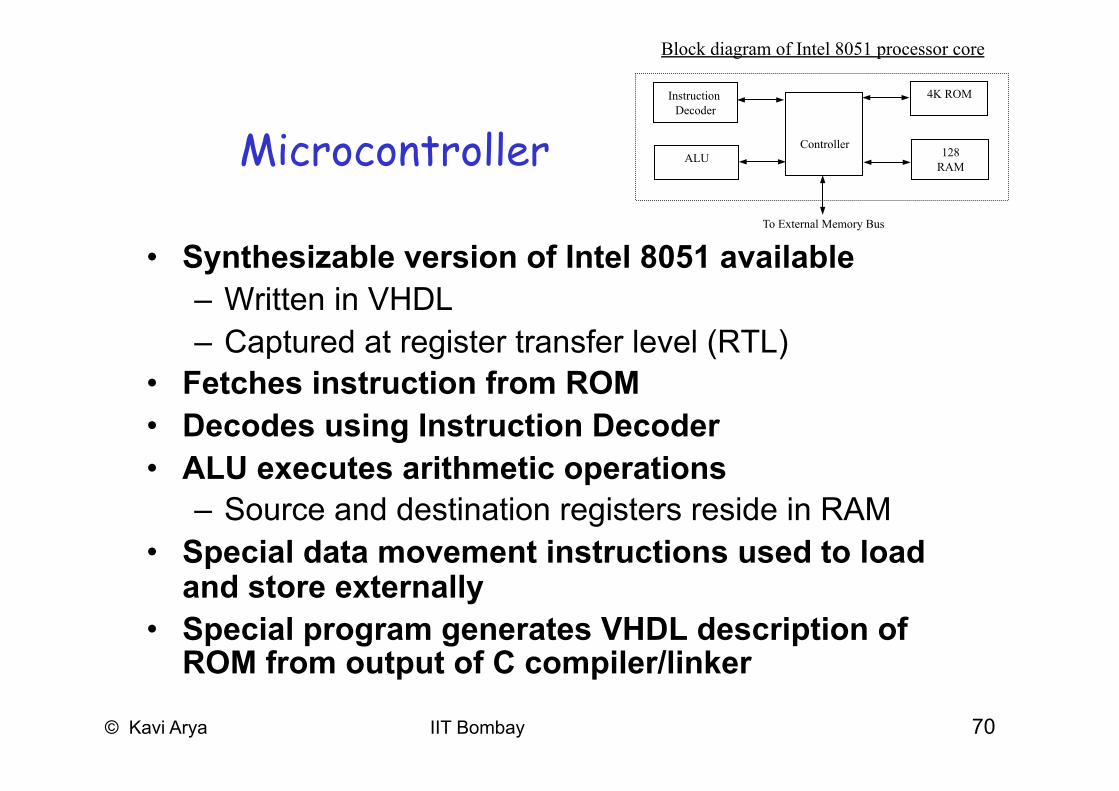
Block diagram of Intel 8051 processor core
© Kavi Arya IIT Bombay 70
Microcontroller
• Synthesizable version of Intel 8051 available – Written in VHDL – Captured at register transfer level (RTL)
• Fetches instruction from ROM • Decodes using Instruction Decoder • ALU executes arithmetic operations
– Source and destination registers reside in RAM • Special data movement instructions used to load
and store externally • Special program generates VHDL description of
ROM from output of C compiler/linker
To External Memory Bus
Controller
4K ROM
128 RAM
Instruction Decoder
ALU
Block diagram of Intel 8051 processor core

© Kavi Arya IIT Bombay 71
UART • UART in idle mode until invoked
– UART invoked when 8051 executes store instruction with UART’s enable register as target
address • Memory-mapped communication • Lower 8-bits of memory address for RAM • Upper 8-bits of memory address for memory-mapped I/
O devices • Start state transmits 0 indicating start of byte
transmission then transitions to Data state • Data state sends 8 bits serially then transitions to Stop
state, Stop state transmits 1 indicating transmission done then transitions back to idle mode
invoked
I = 8
I < 8
Idle:
I = 0
Start: Transmit LOW
Data: Transmit data(I), then I++
Stop: Transmit HIGH
FSMD description of UART

© Kavi Arya IIT Bombay 72
CCDPP • Hardware implementation of zero-bias
operations • Interacts with external CCD chip
– CCD chip resides external to our SOC mainly because combining CCD with ordinary logic not feasible
• Internal buffer, B, memory-mapped to 8051 • Variables R, C are buffer’s row, column indices • GetRow state reads in one row from CCD to B
– 66 bytes: 64 pixels + 2 blacked-out pixels • ComputeBias state computes bias for that row
and stores in variable Bias • FixBias state iterates over same row
subtracting Bias from each element • NextRow transitions to GetRow for repeat of
process on next row or to Idle state when all 64 rows completed
C = 64
C < 64
R = 64 C = 66
invoked
R < 64
C < 66
Idle: R=0 C=0
GetRow: B[R][C]=Pxl
C=C+1
ComputeBias: Bias=(B[R][11] +
B[R][10]) / 2 C=0
NextRow: R++ C=0
FixBias: B[R][C]=B[R][C]-Bias
FSMD description of CCDPP

© Kavi Arya IIT Bombay 73
Connecting SOC components • Memory-mapped
– All single-purpose processors and RAM are connected to 8051’s memory bus
• Read – Processor places address on 16-bit address bus – Asserts read control signal for 1 cycle – Reads data from 8-bit data bus 1 cycle later – Device (RAM or SPP) detects asserted read control signal – Checks address – Places and holds requested data on data bus for 1 cycle
© Kavi Arya IIT Bombay 74
Connecting SOC components… • Write
– Processor places address/data on address/data bus – Asserts write control signal for 1 clock cycle – Device (RAM or SPP) detects asserted write control signal – Checks address bus – Reads and stores data from data bus

© Kavi Arya IIT Bombay 75
Software • System-level model provides majority of code
– Module hierarchy, procedure names, and main program unchanged
• Code for UART and CCDPP modules must be redesigned – Simply replace with memory assignments
• xdata used to load/store variables over external memory bus
• _at_ specifies memory address to store these variables • Byte sent to U_TX_REG by processor will invoke UART • U_STAT_REG used by UART to indicate its ready for
next byte – UART may be much slower than processor
– Similar modification for CCDPP code • All other modules untouched

© Kavi Arya IIT Bombay 76
Software…
static unsigned char xdata U_TX_REG _at_ 65535; static unsigned char xdata U_STAT_REG _at_ 65534; void UARTInitialize(void) {} void UARTSend(unsigned char d) { while( U_STAT_REG == 1 ) { /* busy wait */ } U_TX_REG = d; }
Rewritten UART module
#include <stdio.h> static FILE *outputFileHandle; void UartInitialize(const char *outputFileName) { outputFileHandle = fopen(outputFileName, "w"); } void UartSend(char d) { fprintf(outputFileHandle, "%i\n", (int)d); }
Original code from system-level model

© Kavi Arya IIT Bombay 77
Analysis • Entire SOC tested on
VHDL simulator – Interprets VHDL descriptions
and functionally simulates execution of system
• Recall program code translated to VHDL description of ROM
– Tests for correct functionality – Measures clock cycles to
process one image (performance)
Power
VHDL simulator
VHDL VHDL VHDL
Execution time
Synthesis tool
gates gates gates
Sum gates
Gate level simulator
Power equation
Chip area
Obtaining design metrics of interest
© Kavi Arya IIT Bombay 78
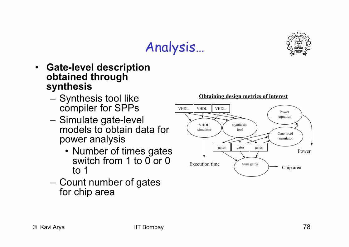
Analysis… • Gate-level description
obtained through synthesis – Synthesis tool like
compiler for SPPs – Simulate gate-level
models to obtain data for power analysis • Number of times gates
switch from 1 to 0 or 0 to 1
– Count number of gates for chip area
Power
VHDL simulator
VHDL VHDL VHDL
Execution time
Synthesis tool
gates gates gates
Sum gates
Gate level simulator
Power equation
Chip area
Obtaining design metrics of interest

© Kavi Arya IIT Bombay 79
Implementation 2: Microcontroller and CCDPP
• Analysis of implementation 2 – Total execution time for processing one image:
• 9.1 seconds – Power consumption:
• 0.033 watt – Energy consumption:
• 0.30 joule (9.1 s x 0.033 watt) – Total chip area:
• 98,000 gates

© Kavi Arya IIT Bombay 80
Implementation 3: Microcontroller and CCDPP/Fixed-Point DCT
• 9.1 seconds still doesn’t meet performance constraint of 1 second
• DCT operation prime candidate for improvement – Execution of implementation 2 shows microprocessor
spends most cycles here – Could design custom hardware like we did for CCDPP
• More complex so more design effort – Instead, will speed up DCT functionality by modifying
behavior
© Kavi Arya IIT Bombay 81
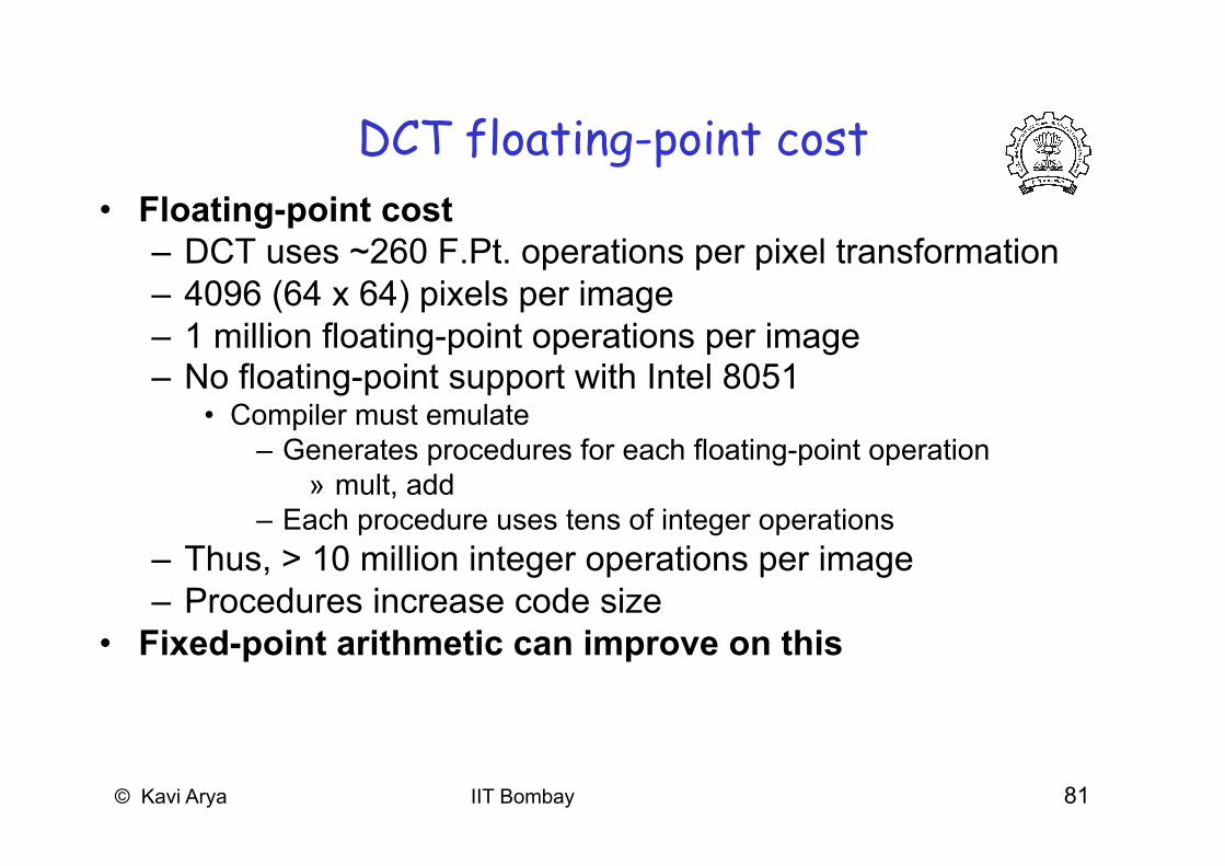
DCT floating-point cost • Floating-point cost
– DCT uses ~260 F.Pt. operations per pixel transformation – 4096 (64 x 64) pixels per image – 1 million floating-point operations per image – No floating-point support with Intel 8051
• Compiler must emulate – Generates procedures for each floating-point operation
» mult, add – Each procedure uses tens of integer operations
– Thus, > 10 million integer operations per image – Procedures increase code size
• Fixed-point arithmetic can improve on this

© Kavi Arya IIT Bombay 82
Fixed-point arithmetic
• Integer used to represent a real number – Constant number of integer’s bits represents
fractional portion of real number • More bits, more accurate the
representation – Remaining bits represent portion of real
number before decimal point

© Kavi Arya IIT Bombay 83
Fixed-point arithmetic…
Translating a real constant to a fixed-point representation – Multiply real value by 2 ^ (# of bits used for fractional part) – Round to nearest integer – E.g., represent 3.14 as 8-bit integer with 4 bits for fraction
• 2^4 = 16 • 3.14 x 16 = 50.24 ≈ 50 = 00110010 • 16 (2^4) possible values for fraction, each represents 0.0625 (1/16) • Last 4 bits (0010) = 2 • 2 x 0.0625 = 0.125 • 3(0011) + 0.125 = 3.125 ≈ 3.14 (more bits for fraction would increase
accuracy)

© Kavi Arya IIT Bombay 84
Fixed-point arithmetic operations • Addition
– Simply add integer representations – E.g., 3.14 + 2.71 = 5.85
• 3.14 → 50 = 00110010 • 2.71 → 43 = 00101011 • 50 + 43 = 93 = 01011101 • 5(0101) + 13(1101) x 0.0625 = 5.8125 ≈ 5.85
• Multiply – Multiply integer representations – Shift result right by # of bits in fractional part – E.g., 3.14 * 2.71 = 8.5094
• 50 * 43 = 2150 = 100001100110 • >> 4 = 10000110 • 8(1000) + 6(0110) x 0.0625 = 8.375 ≈ 8.5094
• Range of real values used limited by bit widths of possible resulting values
© Kavi Arya IIT Bombay 85
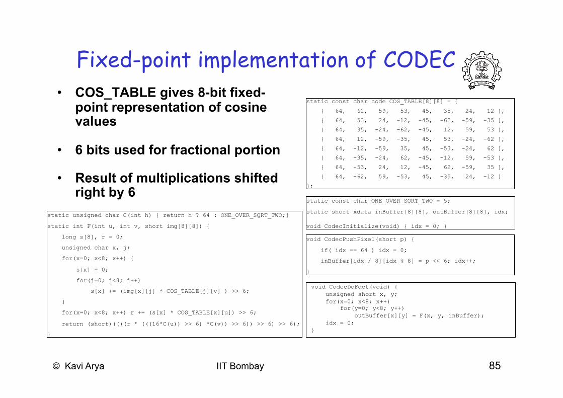
Fixed-point implementation of CODEC • COS_TABLE gives 8-bit fixed-
point representation of cosine values
• 6 bits used for fractional portion
• Result of multiplications shifted right by 6
void CodecDoFdct(void) { unsigned short x, y; for(x=0; x<8; x++) for(y=0; y<8; y++) outBuffer[x][y] = F(x, y, inBuffer); idx = 0; }
static const char code COS_TABLE[8][8] = {
{ 64, 62, 59, 53, 45, 35, 24, 12 },
{ 64, 53, 24, -12, -45, -62, -59, -35 },
{ 64, 35, -24, -62, -45, 12, 59, 53 },
{ 64, 12, -59, -35, 45, 53, -24, -62 },
{ 64, -12, -59, 35, 45, -53, -24, 62 },
{ 64, -35, -24, 62, -45, -12, 59, -53 },
{ 64, -53, 24, 12, -45, 62, -59, 35 },
{ 64, -62, 59, -53, 45, -35, 24, -12 }
};
static const char ONE_OVER_SQRT_TWO = 5;
static short xdata inBuffer[8][8], outBuffer[8][8], idx;
void CodecInitialize(void) { idx = 0; }
static unsigned char C(int h) { return h ? 64 : ONE_OVER_SQRT_TWO;}
static int F(int u, int v, short img[8][8]) {
long s[8], r = 0;
unsigned char x, j;
for(x=0; x<8; x++) {
s[x] = 0;
for(j=0; j<8; j++)
s[x] += (img[x][j] * COS_TABLE[j][v] ) >> 6;
}
for(x=0; x<8; x++) r += (s[x] * COS_TABLE[x][u]) >> 6;
return (short)((((r * (((16*C(u)) >> 6) *C(v)) >> 6)) >> 6) >> 6);
}
void CodecPushPixel(short p) {
if( idx == 64 ) idx = 0;
inBuffer[idx / 8][idx % 8] = p << 6; idx++;
}

© Kavi Arya IIT Bombay 86
Implementation 3: Microcontroller and CCDPP/Fixed-Point DCT
• Analysis of implementation 3 – Use same analysis techniques as implementation 2 – Total execution time for processing one image:
• 1.5 seconds – Power consumption:
• 0.033 watt (same as 2) – Energy consumption:
• 0.050 joule (1.5 s x 0.033 watt) • Battery life 6x longer!!
– Total chip area: • 90,000 gates • 8,000 less gates (less memory needed for code)
© Kavi Arya IIT Bombay 87
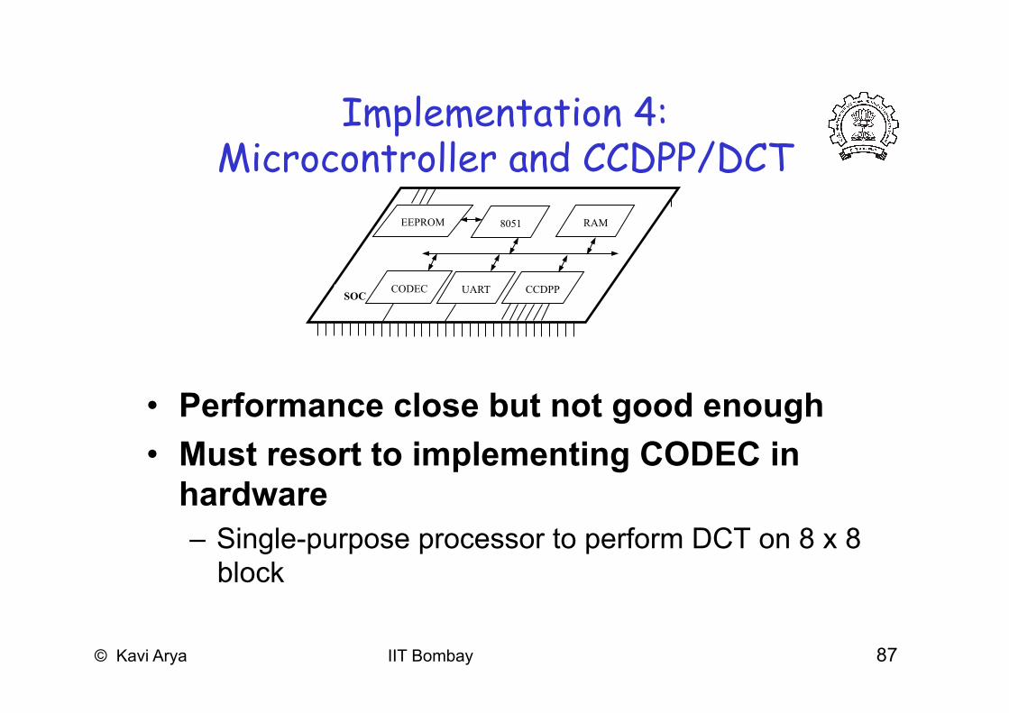
Implementation 4: Microcontroller and CCDPP/DCT
• Performance close but not good enough • Must resort to implementing CODEC in
hardware – Single-purpose processor to perform DCT on 8 x 8
block
8051
UART CCDPP
RAM EEPROM
SOC CODEC
© Kavi Arya IIT Bombay 88
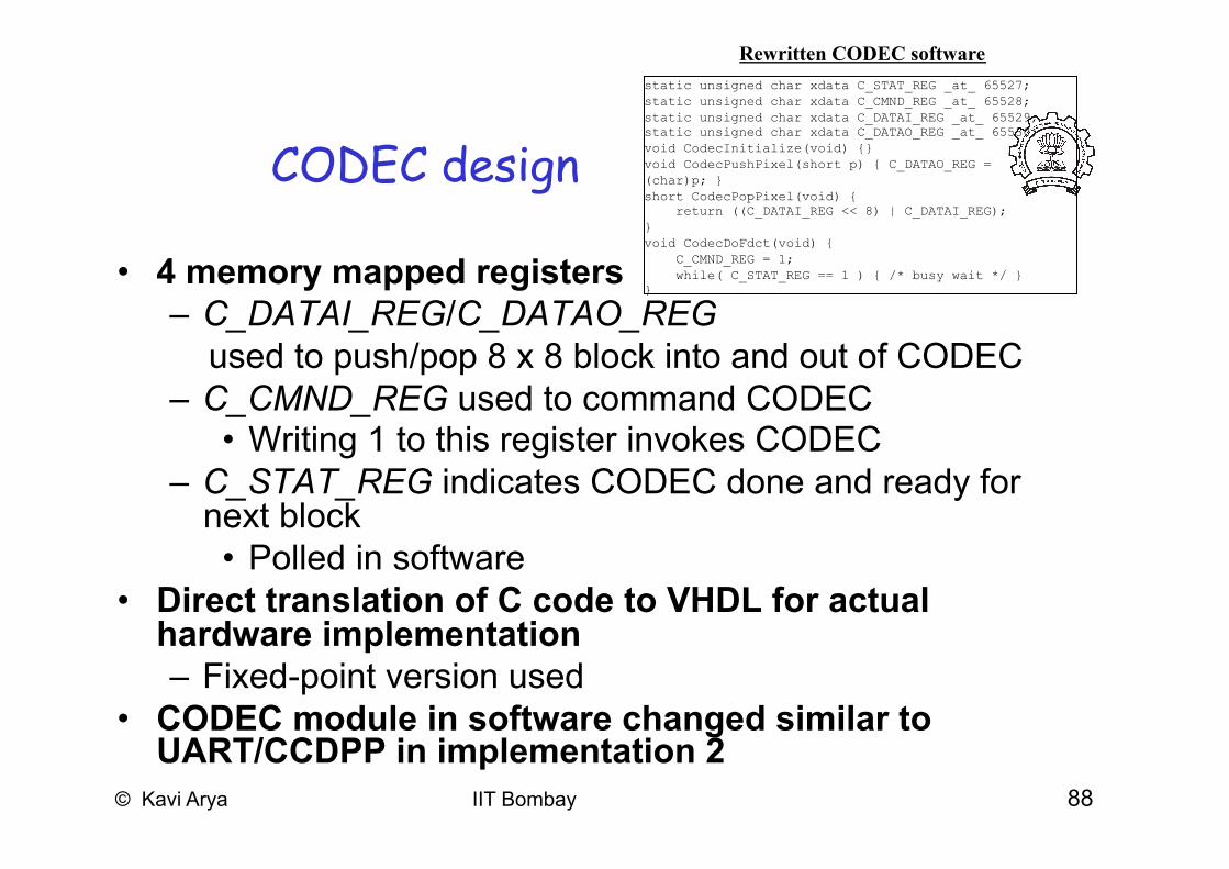
CODEC design
• 4 memory mapped registers – C_DATAI_REG/C_DATAO_REG used to push/pop 8 x 8 block into and out of CODEC – C_CMND_REG used to command CODEC
• Writing 1 to this register invokes CODEC – C_STAT_REG indicates CODEC done and ready for
next block • Polled in software
• Direct translation of C code to VHDL for actual hardware implementation – Fixed-point version used
• CODEC module in software changed similar to UART/CCDPP in implementation 2
static unsigned char xdata C_STAT_REG _at_ 65527; static unsigned char xdata C_CMND_REG _at_ 65528; static unsigned char xdata C_DATAI_REG _at_ 65529; static unsigned char xdata C_DATAO_REG _at_ 65530; void CodecInitialize(void) {} void CodecPushPixel(short p) { C_DATAO_REG = (char)p; } short CodecPopPixel(void) { return ((C_DATAI_REG << 8) | C_DATAI_REG); } void CodecDoFdct(void) { C_CMND_REG = 1; while( C_STAT_REG == 1 ) { /* busy wait */ } }
Rewritten CODEC software

© Kavi Arya IIT Bombay 89
Implementation 4: Microcontroller and CCDPP/DCT
• Analysis of implementation 4 – Total execution time for processing one image:
• 0.099 seconds (well under 1 sec) – Power consumption:
• 0.040 watt • Increase over 2 and 3 because SOC has another
processor – Energy consumption:
• 0.00040 joule (0.099 s x 0.040 watt) • Battery life 12x longer than previous implementation!!
– Total chip area: • 128,000 gates, significant increase over previous
implementations
© Kavi Arya IIT Bombay 90
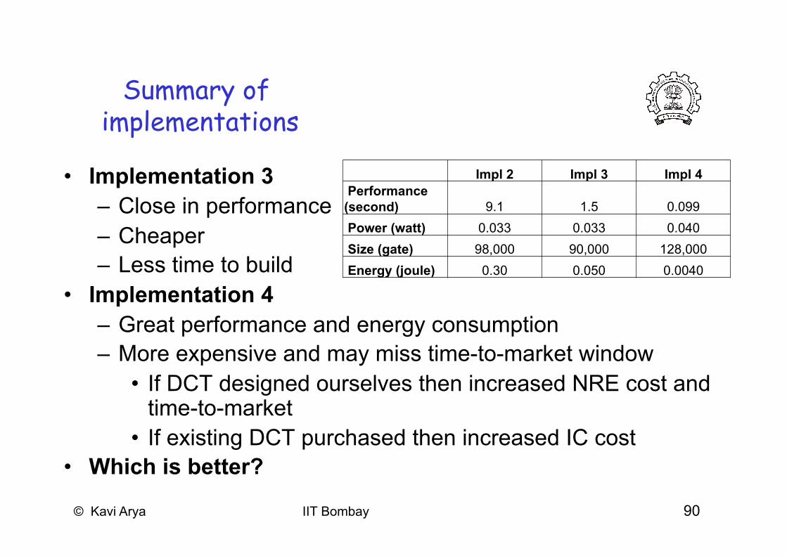
Summary of implementations
• Implementation 3 – Close in performance – Cheaper – Less time to build
• Implementation 4 – Great performance and energy consumption – More expensive and may miss time-to-market window
• If DCT designed ourselves then increased NRE cost and time-to-market
• If existing DCT purchased then increased IC cost • Which is better?
Impl 2 Impl 3 Impl 4 Performance (second) 9.1 1.5 0.099 Power (watt) 0.033 0.033 0.040 Size (gate) 98,000 90,000 128,000 Energy (joule) 0.30 0.050 0.0040
© Kavi Arya IIT Bombay 91
Digital Camera -- Summary
• Digital camera example – Specifications in English and executable language – Design metrics: performance, power and area
• Several implementations – Microcontroller: too slow – Microcontroller and coprocessor: better, but still too slow – Fixed-point arithmetic: almost fast enough – Additional coprocessor for compression: fast enough, but
expensive and hard to design – Tradeoffs between hw/sw – the main lesson of this course!

© Kavi Arya IIT Bombay 92
Examples of Embedded Systems
We looked at details of • A simple Digital Camera
We will study microcontroller prog. with
• TI TIVA Microcontroller based on ARM Cortex (to be studied in microcontroller workshop)
The world gets exciting… • Apple iPad, intelligent
transportation systems, service robots, …


![Wordnet-Affect [IIT-Bombay]](https://img.pdfslide.net/doc/110x75/55503cebb4c90580748b4770/wordnet-affect-iit-bombay.jpg)


