Embed Size (px)
Citation preview
CSALF-Q: A Bricolage Algorithm for Anisotropic Quad Mesh Generation
CSALF-Q: A Bricolage Algorithm for Anisotropic Quad Mesh
Generation
Nilanjan Mukherjee
Meshing & Abstraction Group
Digital Simulation Solutions
Siemens PLM Software
SIEMENS 2000 Eastman Dr., Milford, Ohio 45150 USA
Abstract: “Bricolage”, a multidisciplinary term used extensively in visual arts, anthropology and
cultural studies, refers to a creation that borrows elements from a diverse range of existing de-
signs. The term is applied here to describe CSALF-Q, a new automatic 2D quad meshing algo-
rithm that combines the strengths of recursive subdivision, loop-paving and transfinite interpola-
tion to generate surface meshes that are anisotropic yet boundary structured, robust yet sensitive
to size fields and competitive in performance. This algorithm is based on the understanding of
boundary loops which are initially meshed recursively with a new, boundary based “loop-paving”
technique that balances anisotropy and mesh quality. The remaining interior domain is filled out
by a symbiotic process that shuttles between recursive subdivision, transfinite interpolation and
loop-paving in an efficient manner. The mesh is finally cleaned and smoothed. Loop-fronts are
classified and rule sets are defined for each, to aid optimum point placement. Stencils used for
loop-closure are presented. Results are presented that compare both local and global element
quality of meshes generated by the new algorithm with that of TQM (TriaQua Mesher) which is
also known to handle variegated sizemaps.
Keywords: subdivision, tri-qua mesher, paving, transfinite, mapped, flattening, loop,
loop-paving, parameterization, quadrilateral.
1 Introduction
Unstructured quadrilateral and hex mesh generation of a large gamut of industrial
problems ranging from automotive, aerospace, electronic and appliance structures and
thermal and fluid flow problems continue to be a key pre-processing step leading to the
complex analyses performed for design validation. In the industry today, we continue to
faithfully use just a handful of quad mesh generation algorithms. Added to the existing
complexity of engineering demands and interaction problems there is a need to create hy-
brid meshes that capture quintessential properties of several mesh generation algorithms,
thus enabling the application engineer or analyst to produce meshes that largely meet
both diverse local and global requirements. This "hybridity", called for thus, is defined in
two ways - first, a mix of elements (quad or hex-dominant meshes) and secondly

Nilanjan Mukherjee
quad/hex or quad/hex-dominant meshes confronted with stringent needs of variegated lo-
cal and global size fields thus requiring challenging anisotropy.
2. Past Research
Owen [1] and Frey and George [2] present detailed overviews on unstructured
meshing algorithms both from historical and practical perspectives. The basic work on
unstructured mesh generation with quadrilaterals could be classified into the following:
1. Transfinite methods
2. Paving or Advancing front type methods
3. Quadtree methods
4. Subdivision or domain decomposition methods
5. Medial Axis methods
6. Sphere/ball/circle packing methods
This paper will only focus on paving, transfinite and subdivision algorithms.
2.1 Advancing Front Methods
The advancing front approach to domain triangulation was introduced by Marcum [3].
Ted Blacker and Stephenson [4] published their ground breaking work on a quadrilateral
advancing front approach they called Paving. Paving and advancing front meshes guaran-
tee a boundary conforming mesh with a very high quality. However, they do not guaran-
tee a “controllable layered mesh". There may not exist a completely structured layer of
elements around boundary loops - as a result properties of such layers cannot be user-
controlled. Staten et al extended the unstructured paving approach to 3D which they
called "plastering" [5]. Earlier White and Kinney [6] had attempted to progress a single
element row until collision occurs. Although an interesting approach, the method does
not help to improve quad element quality and nor guarantee controllable structured layers
of high quality quads near interior boundaries. With triangles however, Pirzadeh [7] pro-
vided an algorithm to advance the boundary layers in a controlled and structured manner.
Peraire et. al [8] made another important contribution in this class of problems by laying
down the essential 3D Euler equations for boundary layer advancement. Very recently,
Moreno et al [9] reported an improvisation of the paving algorithm that creates conti-
nuous and homogeneous curved triangular and quadrilateral meshes directly on NURBS
geometry. Another strong limitation of the paving algorithm is its inability to handle
complex sizemaps not making it the obvious choice for highly anisotropic quadrilateral
meshes.
2.2 Subdivision Methods
Subdivision algorithms dissect a given polygon into either a simultaneous set of con-
vex domains or a recursively split dynamic domain. The main idea here is to generate a
best-split-line to subdivide the polygon into smaller areas that are pre-dominantly convex.
The polygonal postulate that states that a convex polygon, when linearly truncated, leads
to only convex domains, serves as the basis for this approach. Since convex polygon do-
main yields a dominant convex mesh, the mesh quality produced by these algorithms is
CSALF-Q: A Bricolage Algorithm for Anisotropic Quad Mesh Generation
enviably high. It needs to be categorically pointed out that subdivision methods pre-
existed advancing-front types and some of these provided the first automatic method of
discretizing areas for the purpose of finite element analyses. There are two basic ap-
proaches with subdivision - (i) recursive subdivision and (ii) simultaneous subdivision.
Each one has its strength and limitations. Sluiter and Hansen [10] and Schoofs et al. [11]
made pioneering contributions in this area of recursive subdivision. Sluiter’s work was
later revisited and revised by many including Talbert and Parkinson [12], Sarrate and
Huerta [13] and Cabello [14]. The strength of these algorithms lie in their robustness in
handling complex shapes, constraints, sizemaps and efficiency. The meshes produced
have reasonable good quality. Mezentsev et al [15] described a generic approach to un-
structured mesh generation on subdivision geometry. Berzin et al [16] developed in re-
cent years a subdivision technique based on Modified Butterfly interpolation scheme for
triangular mesh generation. Barry Joe [17], in his public domain code GeomPack, pro-
poses a method to proceed from a simultaneous set of convex sub-domains. A similar
methodology was proposed by Nowottny [18].
3. CSALF-Q
Automotive and aerospace structural analysts from the engine and transmission
areas have long voiced their need for layered boundary conforming meshes in generally
unstructured domains. To be able to have suitable control on the parameters of these
layered meshes is a key requirement. Another need has been transitioning meshes, well-
adapted to surface curvature and local constraints. User control, especially in the boun-
dary layers is also key to these analyses.
In a 1962 essay titled “The Savage Mind” [19] legendary French anthropologist
Claude Lévi-Strauss used the word bricolage to mean “make creative and resourceful use
of whatever materials are at hand”. Since then, the term “bricolage” has been used
extensively in a large range of disciplines including science, visual arts and engineering
to suggest construction or creation of a work from a diverse range of existing designs or
algortihms. In the present paper, a similar effort is made to create a new hybrid quadrila-
teral mesher in 2D that combines two mutually complimentary aspects of unstructured
meshing. One of them is a recursive subdivision algorithm. The other is a new paving
loop-front method. The original recursive subdivision algorithm TriQuaMesh, reported
more than three decades back by Sluiter and Hansen [10] emphasizes on a recursive con-
tour or loop-splitting algorithm that produces reasonably good quality quad meshes in an
automatic mode. An industrial version of the algorithm has been improvised in the I-
DEAS and NX softwares. The algorithm has had more than a quarter-century long indus-
trial mileage and is well known as one of the most general purpose and robust surface
meshing codes in the industry. However, this technique does not create boundary-
structured quad meshes like paving. Paving, on the other hand, does not adapt to large
size transitions very effectively and is known to be susceptible to the presence of a large
number of interior point constraints – a dire necessity for body-in-white meshing in the
car industry. In this paper, the traditional paving technique of Blacker and Stephenson [4]
is improvised to create an advancing loop-paving-loop algorithm that is coupled to the
modified recursive subdivision technique. This results in CSALF (Combined Subdivision
And Loop-Front) mesher. A triangular version of the same algorithm has been recently
reported elsewhere [20]. It is a bricolage mesher that can produce anisotropic unstruc-
tured meshes that are predominantly boundary structured. The user can optionally control
Nilanjan Mukherjee
layer advancement in terms of number and thickness. The mesh, however, has an overall
unstructured nature and elegantly adapts to sharply varying size fields and can honor any
number of valid interior point constraints.
Given a precisely discretized (isotropic or anisotropic) polygonal boundary,
representing the area to be meshed, the proposed hybrid mesher algorithm initiates the
meshing process with an advancing loop front method. The initial goal is to generate
high-quality boundary conforming layered meshes. As the layer penetrates into the mesh
area, new loops are created each time, reducing the mesh area. As the new loops begin
overlapping, the advancing loop front algorithm is terminated and the subdivision algo-
rithm is activated as shown in Fig. 1.
At this point, all loops are connected into a single continuous contour following pro-
cedures described by Cabello [14]. All interior point constraints are treated as a single-
point loop. Next, the contour is split recursively by determining a best-splitting line. The
splitting line dissects the compound contour into a left sub-contour and a right sub-
contour (Fig 4.) Each left sub-contour is now recursively split into two children sub-
contours - one on the right and a another one on the left. The split lines are so chosen that
they make angles nearing 90 degrees with the contour boundaries.
Recursive splitting finally fills out the mesh area.
The overall algorithmic logic can be expressed in two phases represented by the follow-
ing twin-algorithms –
ALGORITHM I : Generating a single continuous contour-loop
1. The 3D facetted surface is first flattened into a 2D domain following domain genera-
tion procedures as discussed recently by Beatty and myself [21].
2. Face-interior features like holes, scars (loops with repeated edges) and convex-
shaped inner loops are identified.
3. A local and global size-map is developed over the 2D domain. Number of paving
layers around inner loops are determined based on feature recognition, proximity to
other boundaries, global size-map and local user-driven size criteria.
4. Nodes are generated on the boundary of the face accordingly and a triangular back-
ground mesh (based on the TQM algorithm, [15] ) is created for size-sampling.
5. A mesh area is defined in a 2D domain with N meshed loops
6. The N meshed loops represent the area boundary and are unique and non-intersecting
7. While loops are non-intersecting and number of layers defined on various loops are
not exhausted
{ 7a. Cycle all N loops, inner loops first, the outer
loop last
{
7aa. Activate the loop-paving-front
algorithm on the i-th loop
7ab. Check if the new loop self-intersects. If
it does, turn off the loop-paver
for this loop and go to 7ac.
7ac. Continue the cycle, go to the next loop
}
}
8. Connect all N loops into a continuous contour C

CSALF-Q: A Bricolage Algorithm for Anisotropic Quad Mesh Generation
ALGORITHM II : The Symbiotic Triad
To fill the single continuous contour-loop C with a quad or quad-dominant mesh, three
meshing algorithms are used in tandem in a symbiotic manner - Recursive Subdivision,
Transfinite Interpolation and Loop-Paving following a stratagem described by the flow-
chart in Fig.1. As soon as the contourloop is split, it results in two child contourloops - a
left loop CL and a right loop CR.
If the left contourloop CL is convex, meets the sizemap limitations (as explained
in section 7) and is map-meshable, the transfinite mesher is called. Otherwise it is loop-
paved, provided all apriori and posteriori checks pass. The new loop produced by loop-
paving, or the unaffected original loop is returned to the recursive subdivider. This sym-
biotic handling of the loops continues between the three meshing algorithms until there is
no right loop and the left loop is completely filled. The right loop is now split into two
loops again and the process is repeated until the complete mesh-area is filled out. Some
regions of the 2D mesh generated is topologically cleaned by a mesh cleaner [22] and
smoothed using a variational smoother [23].
4. Paving Loop-Front
The paving loop front approach differs from traditional advancing fronts in the sense that
a series of “loop fronts” are considered for mesh advancement. When all loop fronts of a
loop are advanced successfully, a new loop results that imitates and preserves the profile
of the starting loop. This results in a perfectly layered mesh near inner and outer bounda-
ries of the mesh area – a feature which is often preferred by structural and computational
fluid dynamics analysts. Each loop front as shown in Fig 2., consists of a real segment
BC and a virtual segment AB (represented by the previous element edge on the loop).
The virtual segment represents a trailing edge of the real segment of the previous loop-
front.
The virtual segment helps pave the loop front. The angle , between the real and vir-
tual segments of the loop front is used to characterize the loop front. Table I lists the var-
ious loop fronts supported by the algorithm. Q denotes the new node that is created up-
stream of the loop-front, P denotes the node downstream of the loop-front that mostly
pre-exists (created in certain special cases). All additional new nodes R, S,T and U are
created between P and Q.
4.1 New Node Placement
When a paving loop-front is advanced, the new or optimal node placement depends on the type
of the loop-front. For an flat paving loop-front, the position of the only new node Q can be ex-
pressed as
rQ = rB + Vt.g (1)
where rB is the position vector of node B, Vt is the bisector of angle ABC and grading g is as-
sumed to be the harmonic mean of the sizes at the nodes defining the loop-front.
g = 3gAgBgC/sin(θ/2)(gAgB + gBgC + gCgA) (2)
gA, gB, gC are the grading values at nodes A,B & C.

Nilanjan Mukherjee
Fig. 1. Flowchart of Symbiotic Triad Algorithm for meshing continuous contourloop C
Fig. 2. A typical paving loop-front
Recursive Sub-
division of con-
tour-loop
Transfinite
Intpl.
Is
CL convex ?
Loop-Paving
Right side loop
CR
Left side loop
CL
Meshed
with
quality?
New loop CN
Old loop CL Meshed
with
quality ?
Continuous
Contourloop C
Yes
Yes
No
No
No
SYMBIOTIC
TRIAD
Yes
Size Variation
limited?
No
Yes
CSALF-Q: A Bricolage Algorithm for Anisotropic Quad Mesh Generation
Table I shows the formulas for positioning the new nodes during loop-paving. For a Right-
Reversal paving loop-front, 3 new nodes (Q,R&S) are created. The angle bisector unit vector is
transformed by ± θ/6 to obtain the translational unit vectors for nodes Q and R. For all nodes that
are diagonally opposite to node B, the grading is multiplied by a factor of √2 to account for or-
thogonality. In a similar manner for a Reversal paving loop-front 5 nodes (Q,R,S,T,U) are
created. The angle bisector unit vector is transformed by ± θ/4 and ± θ/8 to obtain the transla-
tional unit vectors for nodes Q,R and U,S respectively. Each new node is tested for proximity
with its immediate neighbors in an attempt to avoid creating nearly-squished or hourglass-shaped
quads. When such situations arise decision is taken either to merge proximate nodes or complete-
ly reject the loop for paving.
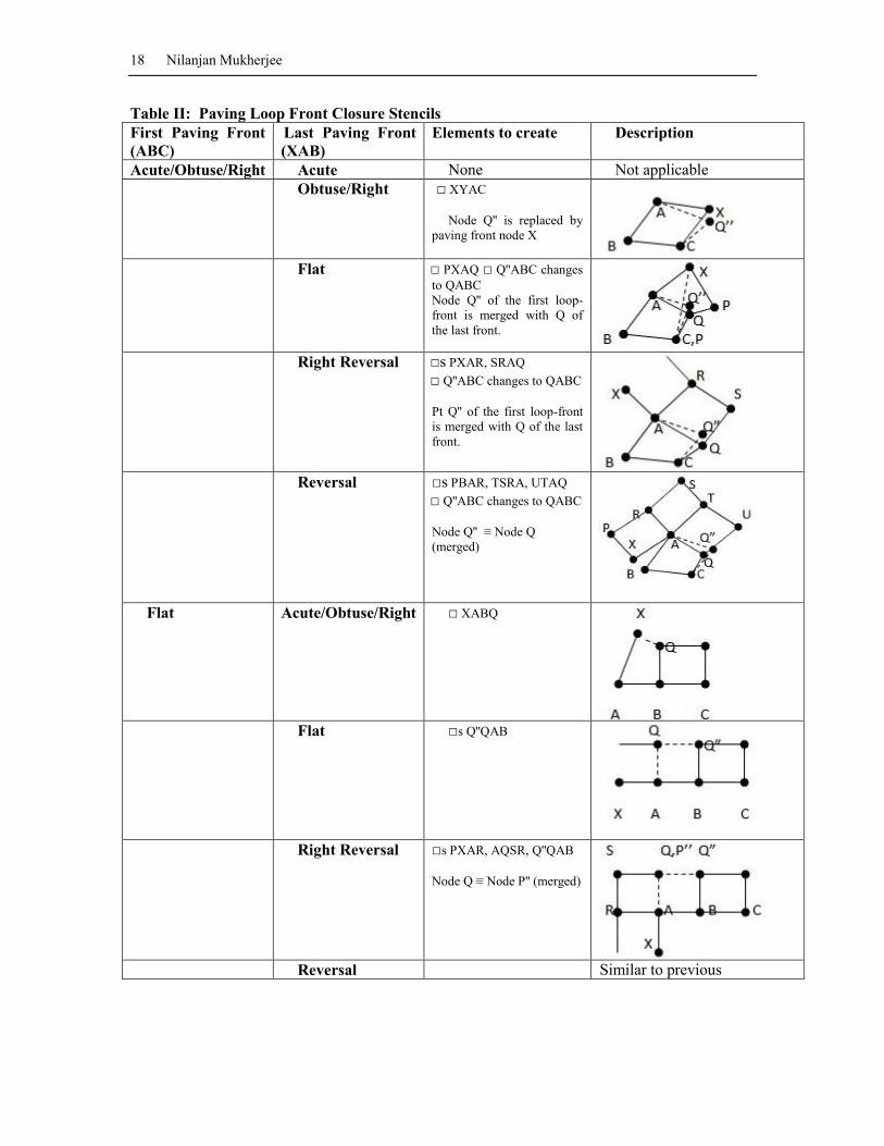
4.2 Loop closure
Loop closing is a delicate affair. Exceptions need to be made to the forward creation theorems (as
illustrated and explained in Table I) for the various paving loop-fronts in this case. Table II lists
the stencils used for each-pair of loop-front types. The terminal loop front is represented by XAB
while the first loop-front is ABC. All nodes marked P'',Q'', R'' etc. refer to the original nodes
created during the advancement of the first front. Nodes P,Q,R,T etc. denote the last loop-fronts
new advancing node positions created at the time of loop closure. To close the loop, 1,2 or 3 ter-
minal elements need to be created based on the pairing type.
After each paving-loop is advanced or paved, the elements and nodes generated in the process are
smoothed using an isoparametric smoother as described by Blacker and Stephenson [4] with a
minor difference in that it is applied to a closed loop of elements and node rings and thus the Di-
richlet and Neumann boundary conditions are placed accordingly.
4.3 Loop Front Evaluators
Loop closing is a delicate affair. Exceptions need to be made to the forward creation theorems (as
illustrated and explained in the Appendix (Table I) for the various loop-fronts in this case. Table
II lists the various stencils used for each-pair of loop-front types. The terminal loop front is
represented by ABC while the first loop-front is BCE. Pt D represents the first new advancing
point of the loop. Pt Q denotes the last new advancing point which, at the time of loop closure,
has already been created. To close the loop, 1 or 2 terminal elements need to be created based on
the pairing type.
Before and after a loop is paved a number of checks are performed, each one for a different pur-
pose. These checks are explained below
4.3.1 Loop Area Shrinkage - With every successful loop-paving, the loop area
shrinks. This check is a posteriori check that is performed on the paved loop to en-
sure the ratio of the loop areas of the new and original loops (An, Ao) do not shrink
below an area tolerance (εA) -
An/Ao > εA (3)
Nilanjan Mukherjee
4.3.2 Loop Perimeter Growth/Shrinkage - The loop perimeter can grow and shrink
as the loop advances. This check is also posteriori and compares the ratio of the pe-
rimeters of the new and original loops (Pn, Po) against a perimeter tolerance (εP) as
described by eqn. (4).
|Pn/Po | > εP (4)
4.3.3 Loop Length Variation: Since paving is more heuristic than recursive subdivi-
sion, the mesh pattern and number of elements tend to vary overtly for small varia-
tions of the global size [24]. Also, in traditional paving wedging and tucking are per-
formed [4] to prevent fronts from shrinking and expanding beyond size limits. With
wedges and tucks, paved meshes often produce diamond shaped quads in the middle
of isotonic flowlines. Certain types of analyses, especially crash analysis (of ve-
hicles), are sensitive to that topology [25]. Therefore, a check is performed apriori
where the rate of variation (dL/ds) of loop lengths (L) along its boundary (s) is kept
below a certain limit (εS).
|dL/ds| < εS (5)
4.3.4 Loop-Front Relative Growth Rate - This posteriori check ensures that the ratio
of the extremums (|dL/ds|max, |dL/ds|min) of the loop-front differential growth rates
are within a specified limit (εG). Any irregular and abrupt loop-front size changes are
avoided during paving so as to ensure that the paved mesh layers are good quality
and regular.
|dL/ds|max/ |dL/ds|min < εG (6)
5. Recursive Subdivision
The recursive subdivision algorithm consists of the following steps-
1. join all loops into a single continuous loop
2. recursively split the continuous loop by a best-split-line
3. determine the best split line
4. estimate the number of nodes to be generated on the split line
5. space the nodes on the split line
6. if no more nodes can be generated construct elements if loop has 3 or 4 nodes only
7. goto step 3 and continue until mesh is done
5.1 Connecting loops
In order to connect all loops to a single continuous loop, a cartesian grid of the global element
size is constructed in the background. Given a mesh area with n loops, these cells are used to
identify a pair of nodes representing the shortest distance between outer loop lo and any inner
loop li along a line whose optimum angular deviation φ (discussed in sect. 5.2) is minimum . The
connecting line is checked for intersection with any other loops. Once this connection is made the
problem now is reduced to one connecting n-1 loops. The process is repeated until it a single con-
tinuous loop results.
5.2 Recursion algorithm
CSALF-Q: A Bricolage Algorithm for Anisotropic Quad Mesh Generation
The recursive subdivision algorithm takes a single 2D contourloop defined by a sequence of nodes and
recursively splits it to fill the region. The input contourloop must not be self-intersecting nor have coinci-
dent nodes but can be self-touching. Nodes can also have repeated entry in the loop. The subdivision logic
is described by the following flow-logic
ALGORITHM III : The recursive subdivision logic
While the compound contour is not completely filled (refer Fig. 3b)
{ 1a. Get the best splitting line A that makes an
angle close to 90 degree with the contour.
The splitting line divides the contour into
a sub-contour on the left (CL ) and one on
the right(CR).
1b. while the left sub-contour CL is unfilled
{
Repeat step 1a
}
1c. while the right sub-contour CR stays unfilled
{
Repeat step 1a
}
}
5.3 Selecting the best split line
The split line functional Φ for a split line joining boundary nodes j and k, is expressed as a li-
near combination of normalized parameters, L, φ and ε ( where A1, A2, A3 are constants ).
Φ = A1 L + A2 φ + A3 ε (7)
The normalized length parameter L is given by L = ljk/ld; ljk is the length of the split line jk (as
shown in Fig. 3b), ld is the characteristic length, which is the diagonal of the rectangular box
bounding the mesh area B ≡ [(xmin,ymin) , (xmax, ymax)] and given by
ld2 = (xmax – xmin)
2 + (ymax – ymin)
2 (8)
The normalized split angle φ is expressed as the normalized sum of the deviations of the 4
split angles (shown in Fig. 3b) from the ideal quadrilateral angle π/2.
4
∑ | φi – π/2 |
φ = i=1
_________ (9)
2π
The percentage of length error ε resulting from fitting n nodes on the split line based on the
grading values of sample points is discussed elsewhere [14] in details.
The minimum value of the split line functional gives the best split line. However, many of the
split line candidates in a concave loop are invalid as they fall outside the domain (as shown in
Fig. 3a). A boundary visibility criterion is set up to eliminate these invalid candidates.

Nilanjan Mukherjee
Fig. 3a. An invalid split line JK joining nodes j and k of the single continuous loop.
Based on experience with a large range of mesh areas, a range for the constants (A1 , A2 , A3 )
are heuristically determined [14].
Fig. 3b. A valid split line joining nodes j and k.
5.4 Split line discretization
Split line discretization is extremely critical to the ability of the mesh to adapt to a given size
field. The first step is to determine the number of nodes n, to be generated on a split line. A set of
s sample points is first created on the split line with an uniform spacing. s is calculated as
s = ljk(gj + gk)/2gjgk – 1 (10)
The grading values (gi) at these s sample points are determined from eqn. (11). The grading
distribution along the split line is assumed to be an s+2-polynomial variation of the natural line
coordinate ξ expressed as
gi(ξ) = 1+C1ξi+C2ξi2+C3ξi
3+....Cs+2ξi
s+2 (11)
Substituting the grading values at these s+2 interior sample points, the simultaneous equation family (11)
is solved to determine the coefficients C1,C2,...Cs+2.
For computational efficiency, the grading function could be limited to a quintic order, i.e. s < 4.
g1 = 1+C1ξ1+C2ξ12+C3ξ1
3+....Cs+2ξ1
s+2
g2 = 1+C1ξ2+C2ξ22+C3ξ2
3+....Cs+2ξ2
s+2
..............................................................
gs+2 = 1+C1ξs+2+C2ξs+22+C3ξs+2
3+....Csξs+2
s+2 (12)
The number of nodes n to be generated on the split line jk is estimated as
1
n = ljk/gl where gl = ∫ ξ=0 gξ dξ (13)
φ2 φ1
φ 3 φ 4
j
k
CL
CR
split
line JK
Valid
split
line jk

CSALF-Q: A Bricolage Algorithm for Anisotropic Quad Mesh Generation
In the natural or parametric coordinates of the split line these n nodes will be equally spaced. The loca-
tion of the i-th node on the split line can be expressed in terms of its grading value gi, coordinates of the
previous point p on the same line, and the coordinates of the two end nodes j and k. The following pair of
equations need to be solved to evaluate the location of node i. The split line functional Φ for a split line
joining boundary nodes j and k, is expressed as a linear combination of normalized parameters, L, φ and
ε.
xi2(1+m
2)+2xi[xp + m(c-yp)]+xp
2+(c-yp)
2+gi
2 = 0 (14)
and the equation of the split line
yi = mxi + c (15)
where the slope of the split line is
m = (yk-yj)/(xk-xj) and (16)
c = (xkyj-xjyk)/(xk-xj) (17)
6. Transfinite Interpolation
Transfinite interpolation (extensively discussed by Armstrong and Tam [26], Mitchell [27,28])
and more recently [25]) is optionally employed in convex sub-contour loops only if the size-map variation
within its domain is small. The advantage of TFIs is two fold - a) firstly it is fast and efficient and b) it is
insensitive to small local variations in the size-map and is guaranteed to generate a structured quad mesh
which neither loop-paving nor recursive subdivision can promise.
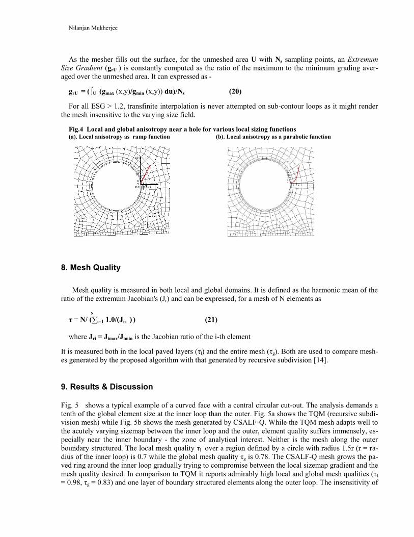
7. Local and Global Anisotropy
The detailed operation of the symbiotic triad explained in Fig. 1 depends on the driving size-map func-
tion defined by the local and global anisotropy requirement. Local anisotropy applies to all face-interior
boundaries or constraints and is defined by two parameters - a) Number of layers desired (nl); and b) A
layer thickness function L(n). Figures 4(a)-(b) depict the meshes around a hole for three different sizing
functions (number of layer desired nl = 5). Many applications, especially structural mechanics, require
boundary-structured graded local meshes and even if the aspect ratio is higher than usual, two rings of
well-shaped quads (Jr < 1.2) minimizes stress solution and smoothening errors. The Fibonacci function
[Li = 1,1,2,3,5; i =0-4;] thus assumes importance. The ramp function, however, is more popular for its
simplicity.
Global anisotropy applies to the entire surface except for interior boundaries with local anisotropic de-
finitions and is defined by a sizing function. The size or grading of the mesh at any interior node is eva-
luated from the size field represented by the background mesh as
g = Г(x,y) (18)
To evaluate the grading at any interior point i (x,y), it’s owner triangle j in the background mesh is identi-
fied by a space hashing mechanism. The grading at point i is thus expressed in terms of the field values at
the vertices of triangle j as
3
gi (x,y) = ∑k=1 Nk gjk (x,y) (19)
gjk (x,y) denote the grading at the vertices of triangle j
Nk represent the shape functions of triangle j
Nilanjan Mukherjee
As the mesher fills out the surface, for the unmeshed area U with Ns sampling points, an Extremum
Size Gradient (grU ) is constantly computed as the ratio of the maximum to the minimum grading aver-
aged over the unmeshed area. It can expressed as -
grU = ( ∫U (gmax (x,y)/gmin (x,y)) du)/Ns (20)
For all ESG > 1.2, transfinite interpolation is never attempted on sub-contour loops as it might render
the mesh insensitive to the varying size field.
Fig.4 Local and global anisotropy near a hole for various local sizing functions (a). Local anisotropy as ramp function (b). Local anisotropy as a parabolic function
8. Mesh Quality
Mesh quality is measured in both local and global domains. It is defined as the harmonic mean of the
ratio of the extremum Jacobian's (Jr) and can be expressed, for a mesh of N elements as
N τ = N/ (∑i=1 1.0/(Jri ) ) (21)
where Jri = Jimax/Jimin is the Jacobian ratio of the i-th element
It is measured both in the local paved layers (τl) and the entire mesh (τg). Both are used to compare mesh-
es generated by the proposed algorithm with that generated by recursive subdivision [14].
9. Results & Discussion
Fig. 5 shows a typical example of a curved face with a central circular cut-out. The analysis demands a
tenth of the global element size at the inner loop than the outer. Fig. 5a shows the TQM (recursive subdi-
vision mesh) while Fig. 5b shows the mesh generated by CSALF-Q. While the TQM mesh adapts well to
the acutely varying sizemap between the inner loop and the outer, element quality suffers immensely, es-
pecially near the inner boundary - the zone of analytical interest. Neither is the mesh along the outer
boundary structured. The local mesh quality τl over a region defined by a circle with radius 1.5r (r = ra-
dius of the inner loop) is 0.7 while the global mesh quality τg is 0.78. The CSALF-Q mesh grows the pa-
ved ring around the inner loop gradually trying to compromise between the local sizemap gradient and the
mesh quality desired. In comparison to TQM it reports admirably high local and global mesh qualities (τl
= 0.98, τg = 0.83) and one layer of boundary structured elements along the outer loop. The insensitivity of
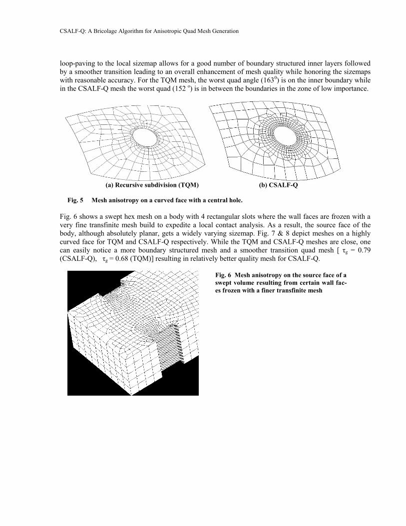
CSALF-Q: A Bricolage Algorithm for Anisotropic Quad Mesh Generation
loop-paving to the local sizemap allows for a good number of boundary structured inner layers followed
by a smoother transition leading to an overall enhancement of mesh quality while honoring the sizemaps
with reasonable accuracy. For the TQM mesh, the worst quad angle (1630) is on the inner boundary while
in the CSALF-Q mesh the worst quad (152 o) is in between the boundaries in the zone of low importance.
(a) Recursive subdivision (TQM) (b) CSALF-Q
Fig. 5 Mesh anisotropy on a curved face with a central hole.
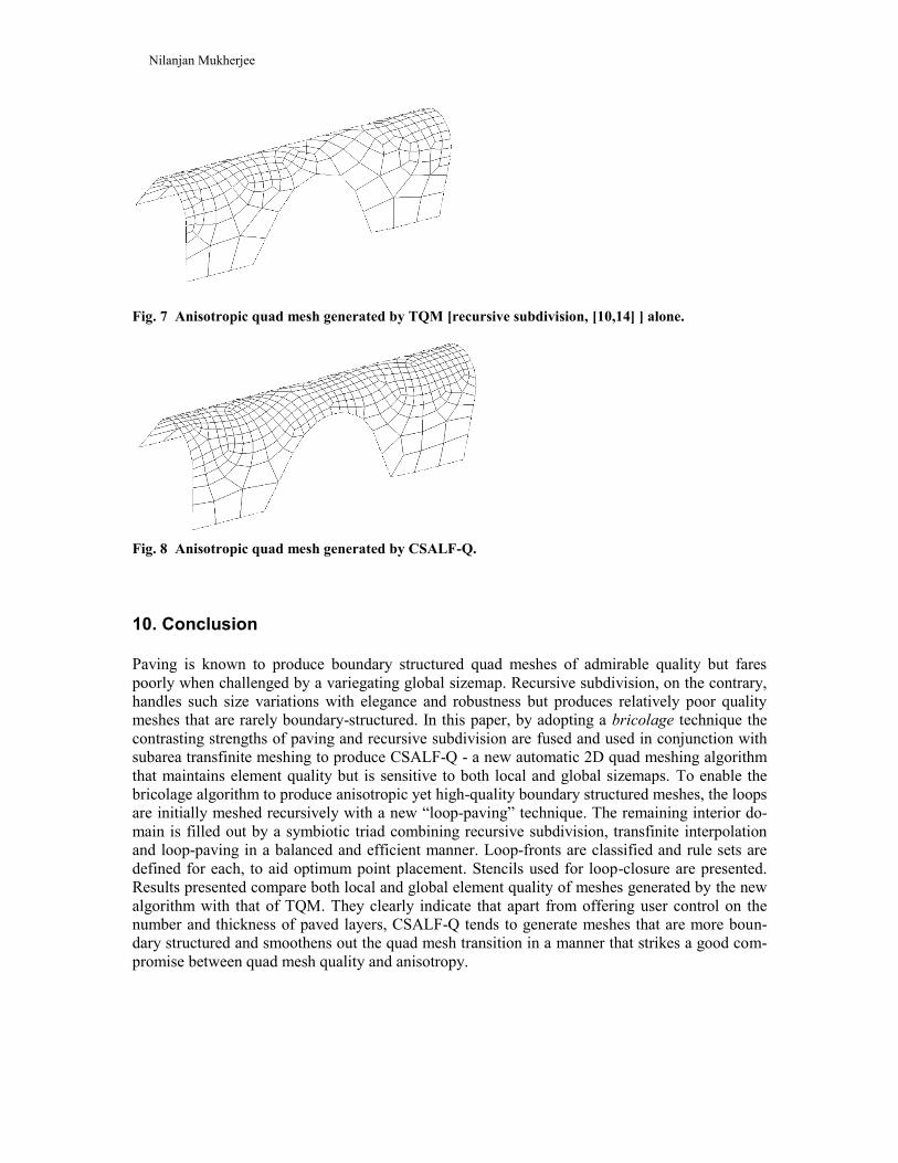
Fig. 6 shows a swept hex mesh on a body with 4 rectangular slots where the wall faces are frozen with a
very fine transfinite mesh build to expedite a local contact analysis. As a result, the source face of the
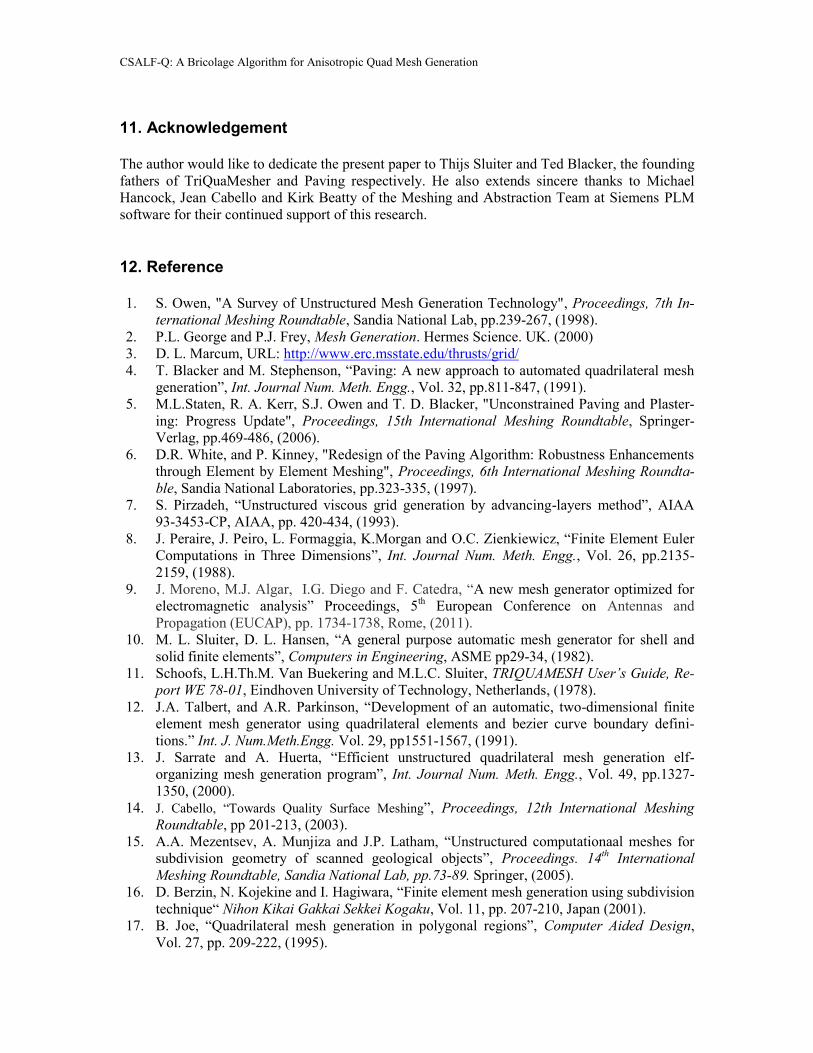
body, although absolutely planar, gets a widely varying sizemap. Fig. 7 & 8 depict meshes on a highly
curved face for TQM and CSALF-Q respectively. While the TQM and CSALF-Q meshes are close, one
can easily notice a more boundary structured mesh and a smoother transition quad mesh [ τg = 0.79
(CSALF-Q), τg = 0.68 (TQM)] resulting in relatively better quality mesh for CSALF-Q.
Fig. 6 Mesh anisotropy on the source face of a
swept volume resulting from certain wall fac-
es frozen with a finer transfinite mesh
Nilanjan Mukherjee
Fig. 7 Anisotropic quad mesh generated by TQM [recursive subdivision, [10,14] ] alone.
Fig. 8 Anisotropic quad mesh generated by CSALF-Q.
10. Conclusion
Paving is known to produce boundary structured quad meshes of admirable quality but fares
poorly when challenged by a variegating global sizemap. Recursive subdivision, on the contrary,
handles such size variations with elegance and robustness but produces relatively poor quality
meshes that are rarely boundary-structured. In this paper, by adopting a bricolage technique the
contrasting strengths of paving and recursive subdivision are fused and used in conjunction with
subarea transfinite meshing to produce CSALF-Q - a new automatic 2D quad meshing algorithm
that maintains element quality but is sensitive to both local and global sizemaps. To enable the
bricolage algorithm to produce anisotropic yet high-quality boundary structured meshes, the loops
are initially meshed recursively with a new “loop-paving” technique. The remaining interior do-
main is filled out by a symbiotic triad combining recursive subdivision, transfinite interpolation
and loop-paving in a balanced and efficient manner. Loop-fronts are classified and rule sets are
defined for each, to aid optimum point placement. Stencils used for loop-closure are presented.
Results presented compare both local and global element quality of meshes generated by the new
algorithm with that of TQM. They clearly indicate that apart from offering user control on the
number and thickness of paved layers, CSALF-Q tends to generate meshes that are more boun-
dary structured and smoothens out the quad mesh transition in a manner that strikes a good com-
promise between quad mesh quality and anisotropy.
CSALF-Q: A Bricolage Algorithm for Anisotropic Quad Mesh Generation
11. Acknowledgement
The author would like to dedicate the present paper to Thijs Sluiter and Ted Blacker, the founding
fathers of TriQuaMesher and Paving respectively. He also extends sincere thanks to Michael
Hancock, Jean Cabello and Kirk Beatty of the Meshing and Abstraction Team at Siemens PLM
software for their continued support of this research.
12. Reference
1. S. Owen, "A Survey of Unstructured Mesh Generation Technology", Proceedings, 7th In-
ternational Meshing Roundtable, Sandia National Lab, pp.239-267, (1998).
2. P.L. George and P.J. Frey, Mesh Generation. Hermes Science. UK. (2000)
3. D. L. Marcum, URL: http://www.erc.msstate.edu/thrusts/grid/
4. T. Blacker and M. Stephenson, “Paving: A new approach to automated quadrilateral mesh
generation”, Int. Journal Num. Meth. Engg., Vol. 32, pp.811-847, (1991).
5. M.L.Staten, R. A. Kerr, S.J. Owen and T. D. Blacker, "Unconstrained Paving and Plaster-
ing: Progress Update", Proceedings, 15th International Meshing Roundtable, Springer-
Verlag, pp.469-486, (2006).
6. D.R. White, and P. Kinney, "Redesign of the Paving Algorithm: Robustness Enhancements
through Element by Element Meshing", Proceedings, 6th International Meshing Roundta-
ble, Sandia National Laboratories, pp.323-335, (1997).
7. S. Pirzadeh, “Unstructured viscous grid generation by advancing-layers method”, AIAA
93-3453-CP, AIAA, pp. 420-434, (1993).
8. J. Peraire, J. Peiro, L. Formaggia, K.Morgan and O.C. Zienkiewicz, “Finite Element Euler
Computations in Three Dimensions”, Int. Journal Num. Meth. Engg., Vol. 26, pp.2135-
2159, (1988).
9. J. Moreno, M.J. Algar, I.G. Diego and F. Catedra, “A new mesh generator optimized for
electromagnetic analysis” Proceedings, 5th European Conference on Antennas and
Propagation (EUCAP), pp. 1734-1738, Rome, (2011).
10. M. L. Sluiter, D. L. Hansen, “A general purpose automatic mesh generator for shell and
solid finite elements”, Computers in Engineering, ASME pp29-34, (1982).
11. Schoofs, L.H.Th.M. Van Buekering and M.L.C. Sluiter, TRIQUAMESH User’s Guide, Re-
port WE 78-01, Eindhoven University of Technology, Netherlands, (1978).
12. J.A. Talbert, and A.R. Parkinson, “Development of an automatic, two-dimensional finite
element mesh generator using quadrilateral elements and bezier curve boundary defini-
tions.” Int. J. Num.Meth.Engg. Vol. 29, pp1551-1567, (1991).
13. J. Sarrate and A. Huerta, “Efficient unstructured quadrilateral mesh generation elf-
organizing mesh generation program”, Int. Journal Num. Meth. Engg., Vol. 49, pp.1327-
1350, (2000).
14. J. Cabello, “Towards Quality Surface Meshing”, Proceedings, 12th International Meshing
Roundtable, pp 201-213, (2003).
15. A.A. Mezentsev, A. Munjiza and J.P. Latham, “Unstructured computationaal meshes for
subdivision geometry of scanned geological objects”, Proceedings. 14th International
Meshing Roundtable, Sandia National Lab, pp.73-89. Springer, (2005).
16. D. Berzin, N. Kojekine and I. Hagiwara, “Finite element mesh generation using subdivision
technique“ Nihon Kikai Gakkai Sekkei Kogaku, Vol. 11, pp. 207-210, Japan (2001).
17. B. Joe, “Quadrilateral mesh generation in polygonal regions”, Computer Aided Design,
Vol. 27, pp. 209-222, (1995).
Nilanjan Mukherjee
18. D. Nowottny, “Quadrilateral mesh generation via geometrically optimized domain decom-
position” Proceedings, 6th Int. Meshing Roundtable, pp. 309-320, (1997).
19. Claude Lévi-Strauss, La Pensée sauvage (Paris, 1962). English translation as The Savage
Mind (Chicago, 1966). ISBN 0-226-47484-4.
20. N. Mukherjee, “A Combined Subdivision and Advancing Loop-Front Surface Mesher (Tri-
angular) for Automotive Structures”, Int. J. Vehicle Structures & Systems, 2(1), pp. 28-37,
(2010).
21. K. Beatty and N. Mukherjee, “Flattening 3D Triangulations for Quality Surface Mesh Gen-
eration”, Proceedings, 17th International Meshing Roundtable, pp 125-139, (2008).
22. P. Kinney, “CleanUp: Improving Quadrilateral Finite Element Meshes”, Proceedings, 6th
International Meshing Roundtable, pp.437-447, (1997).
23. N. Mukherjee, “A hybrid, variational 3D smoother for orphaned shell meshes”, Proceed-
ings., 11th Int. Meshing Roundtable, pp.379-390, (2002).
24. P. Knupp, “Applications of mesh smoothing: Copy, morph, and sweep on unstructured
quadrilateral meshes”, International Journal for Numerical Methods in Engineering,
(1999).
25. Nilanjan Mukherjee, “High Quality Bi-Linear Transfinite Meshing with Interior Point Con-
straints”, Proceedings, 15th International Meshing Roundtable, pp. 309-323,(2006).
26. T. K. H. Tam and C. G. Armstrong, “Finite element mesh control by integer program-
ming”, International Journal for Numerical Methods in Engineering, vol. 36, pp. 2581-
2605, (1993).
27. S. Mitchell, “Choosing corners of rectangles for mapped meshing”, Proceedings, 13th an-
nual symposium on Computational Geometry, pp 87-93, (1993).
28. S. Mitchell, “High Fidelity Interval Assignment”, Proceedings, 6th International Meshing
Roundtable, pp 33-44, (1997).
29. Paving algorithm, UG/Scenario, (1999-2002); NX3, Siemens PLM Software (2004).

CSALF-Q: A Bricolage Algorithm for Anisotropic Quad Mesh Generation
Appendix
Table I: Paving Loop Front Models and Front Advancement Rules
Paving Loop front Type No. of new nodes New Elements
Acute Loop Front
None
None
Right/Obtuse Loop Front
Pt P or Q if this is the first front.
Else, none. Node P comes from
the previous front, Q is same as
P. The obtuse loop-front is diffe-
rentiated from right, because
sometimes based on quality crite-
ria, the obtuse front may be
treated as a flat-front.
□PABC or
□QABC
If element is created, next
front must be skipped.
Flat Loop Front
1 Node Q Position vector of pt Q
rQ = rB + TgQ
T = unit bisector vector of angle
θ
Grading at Q
gQ = 3gAgBgC / sin(θ /2) (gAgB +
gBgC + gCgA)
□QPAB
Right Reversal Loop Front
3-Nodes, Q, R & S rQ = rB + TQgQ rR = rB + TgR rS = rB + TSgS
T= unit bisector vector of angle θ
TQ = T transformed by (-θ/6)
TR = T transformed by (θ/6)
gQ= gR= 3gAgBgC / sin(θ /3)
(gAgB + gBgC + gCgA)
gS = 3√2gAgBgC / sin(θ /3) (gAgB
+ gBgC + gCgA)
□BRPA
□QSRB
Reversal Loop Front
5- Nodes, Q, R, S, T & U rQ = rB + TQgQ rR = rB + TRgR rS = rB + TgS rT = rB + TTgT
rU = rB + TUgU
T = bisector vector of angle θ
TQ = T transformed by (-θ/4)
TU = T transformed by (-θ/8)
TS = T transformed by (θ/8)
TR = T transformed by (θ/4)
gQ = gT = gR= 3gAgBgC / sin(θ /4)
(gAgB + gBgC + gCgA)
gS = gU = 3√2gAgBgC / sin(θ /4)
(gAgB + gBgC + gCgA)
□ABRP
□BTSR
□BQUT
18 Nilanjan Mukherjee
Table II: Paving Loop Front Closure Stencils
First Paving Front
(ABC)
Last Paving Front
(XAB)
Elements to create Description
Acute/Obtuse/Right Acute None Not applicable
Obtuse/Right □ XYAC
Node Q'' is replaced by
paving front node X
Flat □ PXAQ □ Q''ABC changes
to QABC
Node Q'' of the first loop-
front is merged with Q of
the last front.
Right Reversal □s PXAR, SRAQ
□ Q''ABC changes to QABC
Pt Q'' of the first loop-front
is merged with Q of the last
front.
Reversal □s PBAR, TSRA, UTAQ
□ Q''ABC changes to QABC
Node Q'' ≡ Node Q
(merged)
Flat Acute/Obtuse/Right □ XABQ
Flat □s Q''QAB
Right Reversal □s PXAR, AQSR, Q''QAB
Node Q ≡ Node P'' (merged)
Reversal Similar to previous
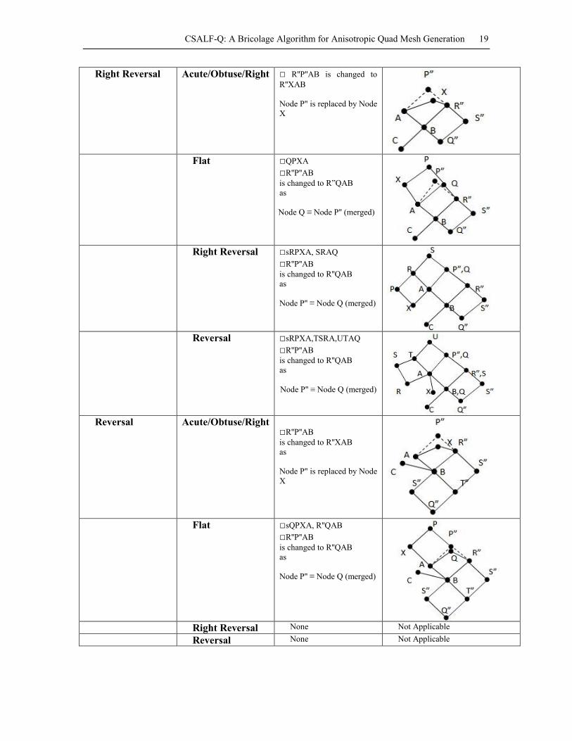
CSALF-Q: A Bricolage Algorithm for Anisotropic Quad Mesh Generation 19
Right Reversal Acute/Obtuse/Right □ R''P''AB is changed to
R''XAB
Node P'' is replaced by Node
X
Flat □QPXA
□R''P''AB
is changed to R”QAB
as
Node Q ≡ Node P'' (merged)
Right Reversal □sRPXA, SRAQ
□R''P''AB
is changed to R''QAB
as
Node P'' ≡ Node Q (merged)
Reversal □sRPXA,TSRA,UTAQ
□R''P''AB
is changed to R''QAB
as
Node P'' ≡ Node Q (merged)
Reversal Acute/Obtuse/Right
□R''P''AB
is changed to R''XAB
as
Node P'' is replaced by Node
X
Flat □sQPXA, R''QAB
□R''P''AB
is changed to R''QAB
as
Node P'' ≡ Node Q (merged)
Right Reversal None Not Applicable
Reversal None Not Applicable

20 Nilanjan Mukherjee