CSC 261/461 –Database Systems Lecture 18

CSC 261/461 – Database SystemsLecture 18

Spring 2018

Announcement

• Quiz 8 WAS due at 2:59 pm today

• Project 2 Part 2 is due tomorrow:– 03/29/2018 (11:59 pm)

TYPES OF INDEXES

Types of Indexing

• Primary Indexes

• Clustering Indexes

• Secondary Indexes

• Multilevel Indexes– Dynamic Multilevel Indexes

• Hash Indexes

• Easy introduction: https://www.tutorialspoint.com/dbms/dbms_indexing.htm

Sorted Files

• Fig 16.7

Recap: No Indexing

Sorted Files (zoomed)

• Fig 16.7

Recap: No Indexing

Primary Indexes: Index for Sorted (Ordered) Files

Example 1

• Suppose that we have an ordered file with r = 30,000 records stored on a disk with block size B = 1024 bytes.

• File records are of fixed size and are unspanned, with record length R = 100 bytes. Also, suppose that the ordering key field of the file is V = 9 bytes long, a block pointer is P = 6 bytes long, and we have constructed a primary index for the file.

• Find out:1. Cost of searching for a record using Binary Search on the data file2. Cost of searching for a record using the index

Example 1 (Part 1)



Find out the cost of searching for a record using Binary Search on the data file

Answer

• Blocking factor:• bfr = ⎣(B/R)⎦ = ⎣(1024/100)⎦ = 10 records per block.

• The number of blocks needed for the file is – b = ⎡(r/bfr)⎤ = ⎡(30000/10)⎤ = 3000 blocks.

• A binary search on the data file would need approximately• ⎡log2 b⎤= ⎡(log23000)⎤ = 12 block accesses.

Example 1 (Part 2)



• Find out the cost of searching for a record using the index

Answer

• The size of each index entry :– Ri= (9 + 6) = 15 bytes,So the blocking factor for the index is bfri= ⎣(B/Ri)⎦ = ⎣(1024/15)⎦ = 68 entries per block.

• The total number of index entries is equal to the number of blocks in the data file, which is 3000.

• The number of index blocks is hence bi= ⎡(ri/bfri)⎤ = ⎡(3000/68)⎤ = 45 blocks.

• To perform a binary search on the index file would need⎡(log2bi)⎤ = ⎡(log245)⎤ = 6 block accesses.

• To search for a record using the index, we need one additional block access to the data file for a total of 6 + 1 = 7 block accesses—an improvement over binary search on the data file, which required 12 disk block accesses.

Clustering Indexes (Index for Sorted (on non-key) Files)

Clustering Indexes (Index for Sorted (on non-key) Files)

Don’t get confused by these two arrows. They are pointing to the same block

Points to the first block that contains the clustering field

Secondary Indexes (on a key field)

• Secondary means of accessing a data file

• File records could be ordered, unordered, or hashed

Note: The data file is a heap file, i.e., not sorted

Secondary Indexes (on a key field)

Note: The data file may be a heap file, i.e., not sorted

Secondary Indexes (on a non-key field)Extra level of indirection

• Provides logical ordering– Though records are not

physically ordered

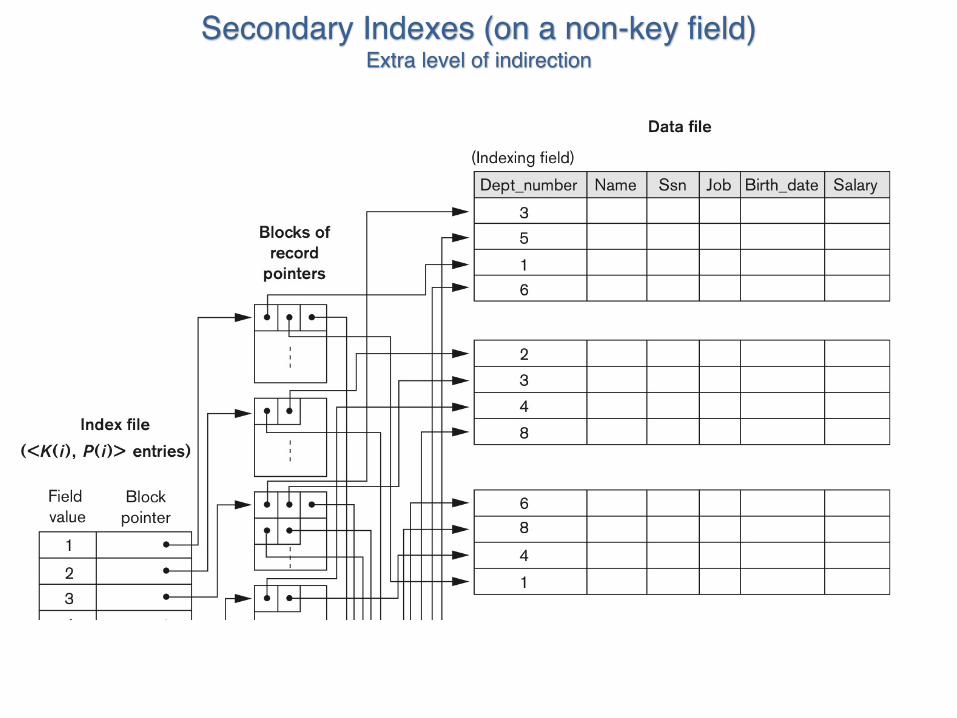
Secondary Indexes (on a non-key field)Extra level of indirection

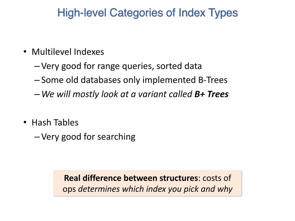
High-level Categories of Index Types

• Multilevel Indexes–Very good for range queries, sorted data– Some old databases only implemented B-Trees–We will mostly look at a variant called B+ Trees

• Hash Tables –Very good for searching

Real difference between structures: costs of ops determines which index you pick and why

MULTILEVEL INDEXES

What you will learn about in this section

1. ISAM

2. B+ Tree

1. ISAM

Primary Indexes: Index for Sorted (Ordered) Files

Review Slide

Review Slide

ISAM

• Indexed Sequential Access Method

– For an index with"!blocks• Earlier: log!b"block

access• Now: log#$b" block

access• (&' = &)*'+,)

ISAM

1. B+ TREES

What you will learn about in this section

1. B+ Trees: Basics

2. B+ Trees: Design & Cost

3. Clustered Indexes

B+ Trees

• Search trees – B does not mean binary!

• Idea in B Trees:–make 1 node = 1 physical page– Balanced, height adjusted tree (not the B either)

• Idea in B+ Trees:–Make leaves into a linked list (for range queries)

https://en.wikipedia.org/wiki/B-tree

B+ Tree Basics

10 20 30

Each non-leaf (“interior”) node has ≥ d and ≤2d keys*

*except for root node, which can have between 1 and 2d keys

Parameter d = degree The minimum number of key an interior node can have

B+ Tree Basics

10 20 30

k < 10

10 ≤ "< 20

20 ≤ "< 3030 ≤ "

The n keys in a node define n+1 ranges

B+ Tree Basics

10 20 30

Non-leaf or internal node

22 25 28

For each range, in a non-leaf node, there is a pointer to another node with keys in that range

B+ Tree Basics

10 20 30

Leaf nodes also have between d and 2d keys, and are different in that:

22 25 28 29

Leaf nodes

32 34 37 38


12 17

B+ Tree Basics

10 20 30

22 25 28 29

Leaf nodes

32 34 37 38


12 17


Their key slots contain pointers to data records

21 22 27 28 30 33 35 371511

B+ Tree Basics

10 20 30

22 25 28 29

Leaf nodes

32 34 37 38


12 17

21 22 27 28 30 33 35 371511


Their key slots contain pointers to data records

They contain a pointer to the next leaf node as well, for faster sequential traversal

B+ Tree Basics

10 20 30

22 25 28 29

Leaf nodes

32 34 37 38


12 17

Note that the pointers at the leaf level will be to the actual data records (rows).

We might truncate these for simpler display (as before)…

Name: JohnAge: 21

Name: JakeAge: 15

Name: BobAge: 27

Name: SallyAge: 28

Name: SueAge: 33

Name: JessAge: 35

Name: AlfAge: 37Name: Joe

Age: 11

Name: BessAge: 22

Name: SalAge: 30

Some finer points of B+ Trees

Searching a B+ Tree

• For exact key values:– Start at the root–Proceed down, to the leaf

• For range queries:–As above–Then sequential traversal

SELECT nameFROM peopleWHERE age = 25

SELECT nameFROM peopleWHERE 20 <= ageAND age <= 30

B+ Tree Exact Search Animation

80

20 60 100 120 140

10 15 18 20 30 40 50 60 65 80 85 90

10 12 15 20 28 30 40 60 63 80 84 89

K = 30?

30 < 80

30 in [20,60)

To the data!

Not all nodes pictured

30 in [30,40)

B+ Tree Range Search Animation

80

20 60 100 120 140

10 15 18 20 30 40 50 60 65 80 85 90

10 12 15 20 28 30 40 59 63 80 84 89

K in [30,85]?

30 < 80

30 in [20,60)

To the data!

Not all nodes pictured

30 in [30,40)

B+ Tree Design

• How large is d?

• Example:– Key size = 4 bytes– Pointer size = 8 bytes– Block size = 4096 bytes

• We want each node to fit on a single block/page– 2d x 4 + (2d+1) x 8 <= 4096 à d <= 170

B+ Tree: High Fanout = Smaller & Lower IO

• As compared to e.g. binary search trees, B+ Trees have high fanout (between d+1 and 2d+1)

• This means that the depth of the tree is small à getting to any element requires very few IO operations!– Also can often store most or all of the B+ Tree

in main memory!

The fanout is defined as the number of pointers to child nodes coming out of a node

Note that fanout is dynamic-we’ll often assume it’s constant just to come up with approximate eqns!

Simple Cost Model for Search

• Let:– f = fanout, which is in [d+1, 2d+1] (we’ll assume it’s constant for our

cost model…)– N = the total number of pages we need to index– F = fill-factor (usually ~= 2/3)

• Our B+ Tree needs to have room to index N / F pages!– We have the fill factor in order to leave some open slots for faster

insertions

• What height (h) does our B+ Tree need to be?– h=1 à Just the root node- room to index f pages– h=2 à f leaf nodes- room to index f2 pages– h=3 à f2 leaf nodes- room to index f3 pages– …– h à fh-1 leaf nodes- room to index fh pages!

à We need a B+ Tree of height h = log! "#

Fast Insertions & Self-Balancing

– Same cost as exact search– Self-balancing: B+ Tree remains balanced (with respect to height)

even after insert

B+ Trees also (relatively) fast for single insertions!However, can become bottleneck if many insertions (if fill-

factor slack is used up…)

Example

• Calculate the order p (order is same as fan-out) of a B+-tree.• Suppose that the search key field is V = 9 bytes long, the block size

is B = 512 bytes, a record pointer is Pr = 7 bytes, and a block pointer is P = 6 bytes.

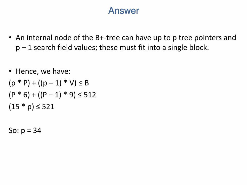
Answer

• An internal node of the B+-tree can have up to p tree pointers and p – 1 search field values; these must fit into a single block.

• Hence, we have:(p * P) + ((p – 1) * V) ≤ B(P * 6) + ((P − 1) * 9) ≤ 512(15 * p) ≤ 521

So: p = 34

Order of the leaf nodes

The leaf nodes of the B+-tree will have the same number of values andpointers, except that the pointers are data pointers and a next pointer. Hence, theorder pleaf for the leaf nodes can be calculated as follows:

(pleaf* (Pr + V)) + P ≤ B(pleaf* (7 + 9)) + 6 ≤ 512(16 * pleaf) ≤ 506

It follows that each leaf node can hold up to pleaf= 31 key value/data pointer combinations,assuming that the data pointers are record pointers.

Insertion

• Perform a search to determine what bucket the new record should go into.

• If the bucket is not full (at most (b-1) entries after the insertion), add the record.

• Otherwise, split the bucket.– Allocate new leaf and move half the bucket's elements to the new bucket.– Insert the new leaf's smallest key and address into the parent.– If the parent is full, split it too.

• Add the middle key to the parent node.– Repeat until a parent is found that need not split.

• If the root splits, create a new root which has one key and two pointers. (That is, the value that gets pushed to the new root gets removed from the original node)

• Note: B-trees grow at the root and not at the leave

b = f = branching factor/ fan-out

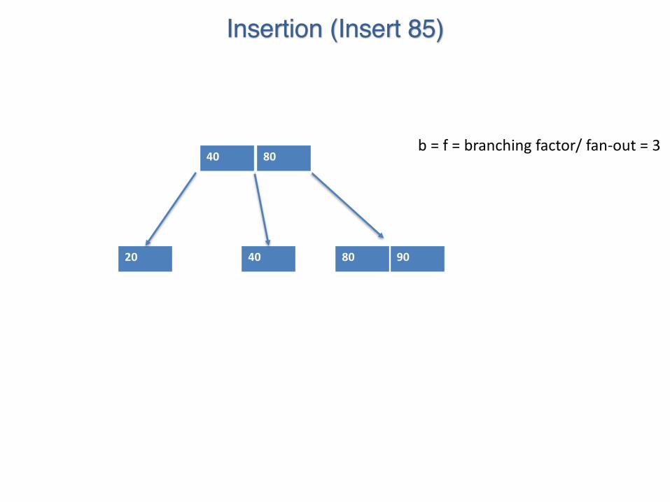
Insertion (Insert 85)

b = f = branching factor/ fan-out = 3

20 40 80 90

40 80



20 40 80 90

40 80

85

This is what we would like. But the maximum number of keys in any node is (3-1) = 2 So, split.



20 40 80

40 80

85

Allocate new leaf and move half the bucket's elements to the new bucket.

90



20 40 80

40 80

85

Insert the new leaf's smallest key and address into the parent.

90

85



20 40 80

40 80

85

This is not allowed, as the parent is full. Need to split

90

85



20 40 80

40

80

85

If the parent is full, split it too. Add the middle key to the parent node.

Repeat until a parent is found that needs no spliting

90

85



20 40 80

40

80

85

If the root splits, create a new root which has one key and two pointers.

(That is, the value that gets pushed to the new root gets removed from the original node)

90

85

Deletion

• Start at root, find leaf L where entry belongs.• Remove the entry.– If L is at least half-full, done!– If L has fewer entries than it should,

• If sibling (adjacent node with same parent as L) is more than half-full, re-distribute, borrowing an entry from it.

• Otherwise, sibling is exactly half-full, so we can merge L and sibling.• If merge occurred, must delete entry (pointing to L or sibling) from

parent of L.• Merge could propagate to root, decreasing height.

• https://www.cs.usfca.edu/~galles/visualization/BPlusTree.html

• The degree in this visualization is actually fan-out f or branching factor b.

Not required for quiz or exam

• Find 86

• Delete it

• Stealing from right sibling (redistribute).• Modify the parent node

• Finally,

Acknowledgement

• Some of the slides in this presentation are taken from the slides provided by the authors.

• Many of these slides are taken from cs145 course offered byStanford University.

Documents

CSC 261/461 –Database Systems Lecture 18