CSC 311: Introduction to Machine Learning · Overview In last lecture we covered PCA, which was an unsupervised learning algorithm. I Its main purpose was to reduce the dimension

CSC 311: Introduction to Machine LearningLecture 9 - k-Means and EM Algorithm

Amir-massoud Farahmand & Emad A.M. Andrews

University of Toronto

Intro ML (UofT) CSC311-Lec9 1 / 41

Overview

In last lecture we covered PCA, which was an unsupervisedlearning algorithm.

I Its main purpose was to reduce the dimension of the data.I In practice, even though data is very high dimensional, it can be

well represented in low dimensions.

This method relies on an assumption that data depends on somelatent variables, which are not observed. Such models are calledlatent variable models.

I For PCA, these corresponds to the code vectors (representation).I Today’s lecture: K-means, a simple algorithm for clustering, i.e.,

grouping data points into clustersI Today’s lecture: Reformulate clustering as a latent variable model,

apply the EM algorithm


Clustering

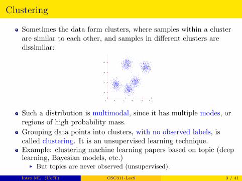
Sometimes the data form clusters, where samples within a clusterare similar to each other, and samples in different clusters aredissimilar:

Such a distribution is multimodal, since it has multiple modes, orregions of high probability mass.

Grouping data points into clusters, with no observed labels, iscalled clustering. It is an unsupervised learning technique.Example: clustering machine learning papers based on topic (deeplearning, Bayesian models, etc.)

I But topics are never observed (unsupervised).


Clustering problem

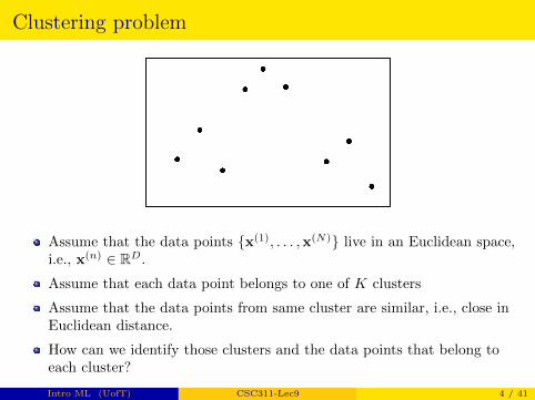
Assume that the data points {x(1), . . . ,x(N)} live in an Euclidean space,i.e., x(n) ∈ RD.

Assume that each data point belongs to one of K clusters

Assume that the data points from same cluster are similar, i.e., close inEuclidean distance.

How can we identify those clusters and the data points that belong toeach cluster?


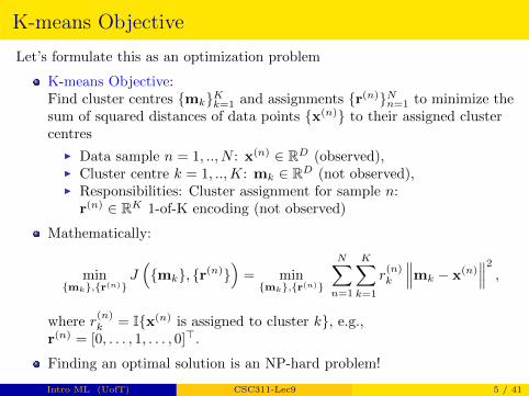
K-means Objective

Let’s formulate this as an optimization problem

K-means Objective:Find cluster centres {mk}Kk=1 and assignments {r(n)}Nn=1 to minimize thesum of squared distances of data points {x(n)} to their assigned clustercentres

I Data sample n = 1, .., N : x(n) ∈ RD (observed),I Cluster centre k = 1, ..,K: mk ∈ RD (not observed),I Responsibilities: Cluster assignment for sample n:

r(n) ∈ RK 1-of-K encoding (not observed)

Mathematically:

min{mk},{r(n)}

J({mk}, {r(n)}

)= min

{mk},{r(n)}

N∑n=1

K∑k=1

r(n)k

∥∥∥mk − x(n)∥∥∥2 ,

where r(n)k = I{x(n) is assigned to cluster k}, e.g.,

r(n) = [0, . . . , 1, . . . , 0]>.

Finding an optimal solution is an NP-hard problem!


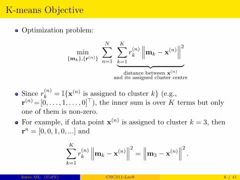
K-means Objective

Optimization problem:

min{mk},{r(n)}

N∑n=1

K∑k=1

r(n)k

∥∥∥mk − x(n)∥∥∥2︸︷︷︸

distance between x(n)

and its assigned cluster centre

Since r(n)k = I{x(n) is assigned to cluster k} (e.g.,

r(n)=[0, . . . , 1, . . . , 0]>), the inner sum is over K terms but onlyone of them is non-zero.

For example, if data point x(n) is assigned to cluster k = 3, thenrn = [0, 0, 1, 0, ...] and

K∑k=1

r(n)k

∥∥∥mk − x(n)∥∥∥2 =

∥∥∥m3 − x(n)∥∥∥2 .


How to Optimize? Alternating Minimization


min{mk},{r(n)}

N∑n=1

K∑k=1

r(n)k

∥∥∥mk − x(n)∥∥∥2

Problem is hard when minimizing jointly over the parameters{mk}, {r(n)}.

But if we fix one and minimize over the other, then it becomes easy.

Doesn’t guarantee the same solution!


Alternating Minimization (Optimizing Assignments)


min{mk},{r(n)}

N∑n=1

K∑k=1

r(n)k ||mk − x(n)||2

Note:

I If we fix the centres {mk}, we can easily find the optimalassignments {r(n)} for each sample n

minr(n)

K∑k=1

r(n)k

∥∥∥mk − x(n)∥∥∥2 .

I Assign each point to the cluster with the nearest centre

r(n)k =

{1 if k = argminj ‖x(n) −mj‖20 otherwise

I E.g. if x(n) is assigned to cluster k̂,

r(n) = [0, 0, ..., 1, ..., 0]>︸︷︷︸Only k̂-th entry is 1


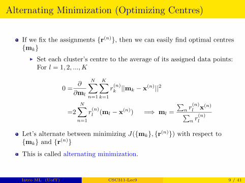
Alternating Minimization (Optimizing Centres)

If we fix the assignments {r(n)}, then we can easily find optimal centres{mk}

I Set each cluster’s centre to the average of its assigned data points:For l = 1, 2, ...,K

0 =∂

∂ml

N∑n=1

K∑k=1

r(n)k ||mk − x(n)||2

=2

N∑n=1

r(n)l (ml − x(n)) =⇒ ml =

∑n r

(n)l x(n)∑n r

(n)l

Let’s alternate between minimizing J({mk}, {r(n)}) with respect to{mk} and {r(n)}

This is called alternating minimization.


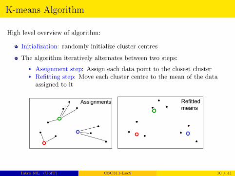
K-means Algorithm

High level overview of algorithm:

Initialization: randomly initialize cluster centres

The algorithm iteratively alternates between two steps:

I Assignment step: Assign each data point to the closest clusterI Refitting step: Move each cluster centre to the mean of the data

assigned to it

Assignments Refitted means


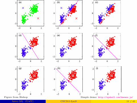
Figure from Bishop Simple demo: http://syskall.com/kmeans.js/


http://syskall.com/kmeans.js/

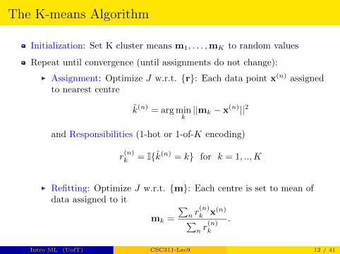
The K-means Algorithm

Initialization: Set K cluster means m1, . . . ,mK to random values

Repeat until convergence (until assignments do not change):

I Assignment: Optimize J w.r.t. {r}: Each data point x(n) assignedto nearest centre

k̂(n) = arg mink||mk − x(n)||2

and Responsibilities (1-hot or 1-of-K encoding)

r(n)k = I{k̂(n) = k} for k = 1, ..,K

I Refitting: Optimize J w.r.t. {m}: Each centre is set to mean ofdata assigned to it

mk =

∑n r

(n)k x(n)∑n r

(n)k

.


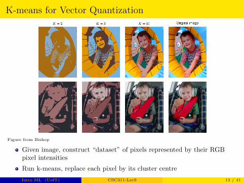
K-means for Vector Quantization

Figure from Bishop

Given image, construct “dataset” of pixels represented by their RGBpixel intensities

Run k-means, replace each pixel by its cluster centre


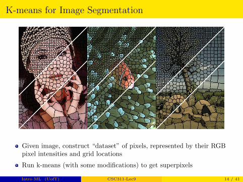
K-means for Image Segmentation

Given image, construct “dataset” of pixels, represented by their RGBpixel intensities and grid locations

Run k-means (with some modifications) to get superpixels


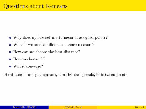
Questions about K-means

Why does update set mk to mean of assigned points?

What if we used a different distance measure?

How can we choose the best distance?

How to choose K?

Will it converge?

Hard cases – unequal spreads, non-circular spreads, in-between points


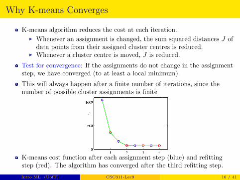
Why K-means Converges

K-means algorithm reduces the cost at each iteration.

I Whenever an assignment is changed, the sum squared distances J ofdata points from their assigned cluster centres is reduced.

I Whenever a cluster centre is moved, J is reduced.

Test for convergence: If the assignments do not change in the assignmentstep, we have converged (to at least a local minimum).

This will always happen after a finite number of iterations, since thenumber of possible cluster assignments is finite

K-means cost function after each assignment step (blue) and refittingstep (red). The algorithm has converged after the third refitting step.


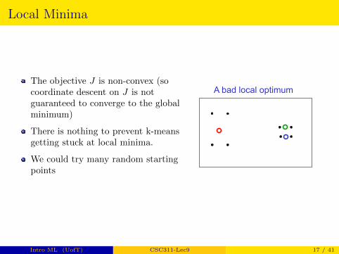
Local Minima

The objective J is non-convex (socoordinate descent on J is notguaranteed to converge to the globalminimum)

There is nothing to prevent k-meansgetting stuck at local minima.

We could try many random startingpoints

A bad local optimum


Soft K-means

Instead of making hard assignments of data points to clusters, we canmake soft assignments. One cluster may have a responsibility of 0.7 for adatapoint and another may have a responsibility of 0.3.

I Allows a cluster to use more information about the data in therefitting step.

I How do we decide on the soft assignments?I We already saw this in multi-class classification:

I 1-of-K encoding vs softmax assignments


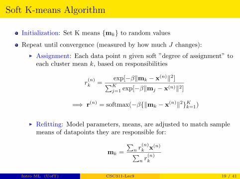
Soft K-means Algorithm

Initialization: Set K means {mk} to random values

Repeat until convergence (measured by how much J changes):

I Assignment: Each data point n given soft ”degree of assignment” toeach cluster mean k, based on responsibilities

r(n)k =

exp[−β‖mk − x(n)‖2]∑Kj=1 exp[−β‖mj − x(n)‖2]

=⇒ r(n) = softmax(−β{‖mk − x(n)‖2}Kk=1)

I Refitting: Model parameters, means, are adjusted to match samplemeans of datapoints they are responsible for:

mk =

∑n r

(n)k x(n)∑n r

(n)k


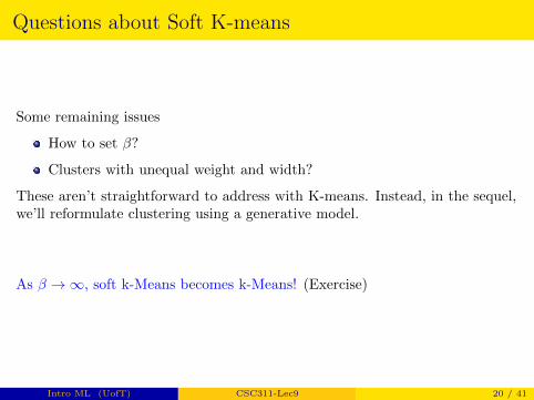
Questions about Soft K-means

Some remaining issues

How to set β?

Clusters with unequal weight and width?

These aren’t straightforward to address with K-means. Instead, in the sequel,we’ll reformulate clustering using a generative model.

As β →∞, soft k-Means becomes k-Means! (Exercise)


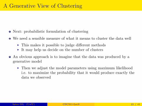
A Generative View of Clustering

Next: probabilistic formulation of clustering

We need a sensible measure of what it means to cluster the data well

I This makes it possible to judge different methodsI It may help us decide on the number of clusters

An obvious approach is to imagine that the data was produced by agenerative model

I Then we adjust the model parameters using maximum likelihoodi.e. to maximize the probability that it would produce exactly thedata we observed


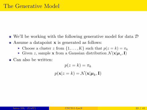
The Generative Model

We’ll be working with the following generative model for data DAssume a datapoint x is generated as follows:

I Choose a cluster z from {1, . . . ,K} such that p(z = k) = πkI Given z, sample x from a Gaussian distribution N (x|µz, I)

Can also be written:p(z = k) = πk

p(x|z = k) = N (x|µk, I)


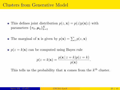
Clusters from Generative Model

This defines joint distribution p(z,x) = p(z)p(x|z) withparameters {πk,µk}Kk=1

The marginal of x is given by p(x) =∑

z p(z,x)

p(z = k|x) can be computed using Bayes rule

p(z = k|x) =p(x | z = k)p(z = k)

p(x).

This tells us the probability that x comes from the kth cluster.


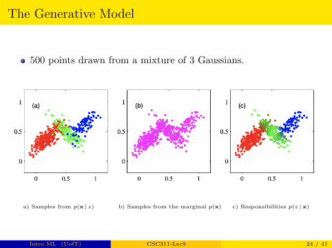
The Generative Model

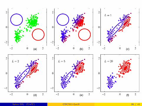
500 points drawn from a mixture of 3 Gaussians.

a) Samples from p(x | z) b) Samples from the marginal p(x) c) Responsibilities p(z |x)


Maximum Likelihood with Latent Variables

How should we choose the parameters {πk,µk}Kk=1?

Maximum likelihood principle: choose parameters to maximizelikelihood of observed data

We don’t observe the cluster assignments z, we only see the data x

Given data D = {x(n)}Nn=1, choose parameters to maximize:

log p(D) =

N∑n=1

log p(x(n))

We can find p(x) by marginalizing out z:

p(x) =

K∑k=1

p(z = k,x) =

K∑k=1

p(z = k)p(x|z = k)


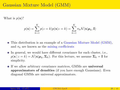
Gaussian Mixture Model (GMM)

What is p(x)?

p(x) =

K∑k=1

p(z = k)p(x|z = k) =

K∑k=1

πkN (x|µk, I)

This distribution is an example of a Gaussian Mixture Model (GMM),and πk are known as the mixing coefficients

In general, we would have different covariance for each cluster, i.e.,p(x | z = k) = N (x|µk,Σk). For this lecture, we assume Σk = I forsimplicity.

If we allow arbitrary covariance matrices, GMMs are universalapproximators of densities (if you have enough Gaussians). Evendiagonal GMMs are universal approximators.


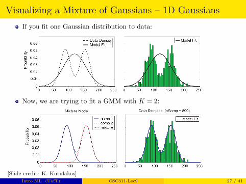
Visualizing a Mixture of Gaussians – 1D Gaussians

If you fit one Gaussian distribution to data:

Now, we are trying to fit a GMM with K = 2:

[Slide credit: K. Kutulakos]


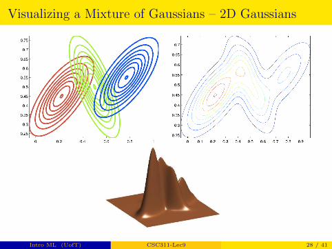
Visualizing a Mixture of Gaussians – 2D Gaussians


Fitting GMMs: Maximum Likelihood

Maximum likelihood objective:

log p(D) =

N∑n=1

log p(x(n)) =

N∑n=1

log

(K∑k=1

πkN (x(n)|µk, I)

)

How would you optimize this w.r.t. parameters {πk,µk}?I No closed-form solution when we set derivatives to 0I Difficult because sum inside the log

One option: gradient ascent. Can we do better?

Can we have a closed-form update?


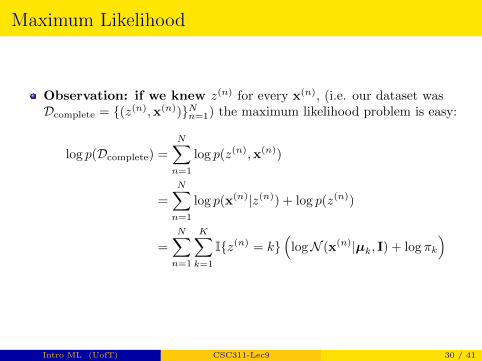
Maximum Likelihood

Observation: if we knew z(n) for every x(n), (i.e. our dataset wasDcomplete = {(z(n),x(n))}Nn=1) the maximum likelihood problem is easy:

log p(Dcomplete) =

N∑n=1

log p(z(n),x(n))

=

N∑n=1

log p(x(n)|z(n)) + log p(z(n))

=

N∑n=1

K∑k=1

I{z(n) = k}(

logN (x(n)|µk, I) + log πk

)


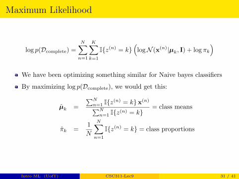
Maximum Likelihood

log p(Dcomplete) =

N∑n=1

K∑k=1

I{z(n) = k}(

logN (x(n)|µk, I) + log πk

)

We have been optimizing something similar for Naive bayes classifiers

By maximizing log p(Dcomplete), we would get this:

µ̂k =

∑Nn=1 I{z(n) = k}x(n)∑Nn=1 I{z(n) = k}

= class means

π̂k =1

N

N∑n=1

I{z(n) = k} = class proportions


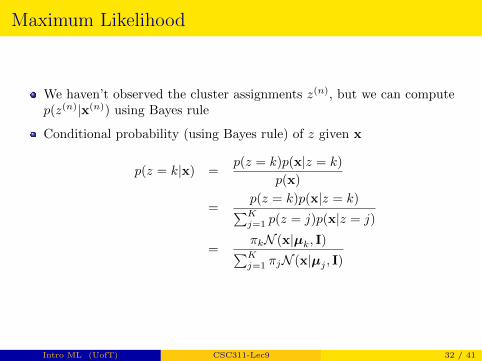
Maximum Likelihood

We haven’t observed the cluster assignments z(n), but we can computep(z(n)|x(n)) using Bayes rule

Conditional probability (using Bayes rule) of z given x

p(z = k|x) =p(z = k)p(x|z = k)

p(x)

=p(z = k)p(x|z = k)∑Kj=1 p(z = j)p(x|z = j)

=πkN (x|µk, I)∑Kj=1 πjN (x|µj , I)


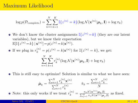
Maximum Likelihood

log p(Dcomplete) =

N∑n=1

K∑k=1

I{z(n) = k}(logN (x(n)|µk, I) + log πk)

We don’t know the cluster assignments I{z(n) =k} (they are our latentvariables), but we know their expectationE[I{z(n) =k} |x(n)]=p(z(n) =k|x(n)).

If we plug in r(n)k = p(z(n) = k|x(n)) for I{z(n) = k}, we get:

N∑n=1

K∑k=1

r(n)k (logN (x(n)|µk, I) + log πk)

This is still easy to optimize! Solution is similar to what we have seen:

µ̂k =

∑Nn=1 r

(n)k x(n)∑N

n=1 r(n)k

π̂k =

∑Nn=1 r

(n)k

N

Note: this only works if we treat r(n)k = πkN (x(n)|µk,I)∑K

j=1 πjN (x(n)|µj ,I)as fixed.


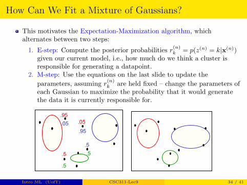
How Can We Fit a Mixture of Gaussians?

This motivates the Expectation-Maximization algorithm, whichalternates between two steps:

1. E-step: Compute the posterior probabilities r(n)k = p(z(n) = k|x(n))

given our current model, i.e., how much do we think a cluster isresponsible for generating a datapoint.

2. M-step: Use the equations on the last slide to update the

parameters, assuming r(n)k are held fixed – change the parameters of

each Gaussian to maximize the probability that it would generatethe data it is currently responsible for.

.95

.5

.5

.05

.5 .5

.95 .05


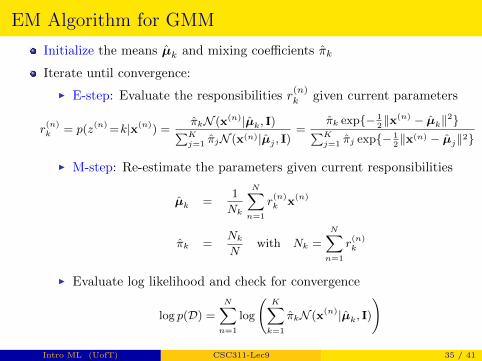
EM Algorithm for GMM

Initialize the means µ̂k and mixing coefficients π̂k

Iterate until convergence:

I E-step: Evaluate the responsibilities r(n)k given current parameters

r(n)k = p(z(n)=k|x(n)) =

π̂kN (x(n)|µ̂k, I)∑Kj=1 π̂jN (x(n)|µ̂j , I)

=π̂k exp{− 1

2‖x(n) − µ̂k‖2}∑K

j=1 π̂j exp{− 12‖x(n) − µ̂j‖2}

I M-step: Re-estimate the parameters given current responsibilities

µ̂k =1

Nk

N∑n=1

r(n)k x(n)

π̂k =Nk

Nwith Nk =

N∑n=1

r(n)k

I Evaluate log likelihood and check for convergence

log p(D) =N∑

n=1

log

(K∑

k=1

π̂kN (x(n)|µ̂k, I)

)



What Just Happened: A Review

The maximum likelihood objective∑N

n=1 log p(x(n)) was hard tooptimize

The complete data likelihood objective was easy to optimize:

N∑n=1

log p(z(n),x(n)) =

N∑n=1

K∑k=1

I{z(n) = k}(logN (x(n)|µk, I) + log πk)

We don’t know z(n)’s (they are latent), so we replaced I{z(n) = k}with responsibilities r

(n)k = p(z(n) = k|x(n)).

That is: we replaced I{z(n) = k} with its expectation underp(z(n)|x(n)) (E-step).


What Just Happened: A Review

We ended up with the expected complete data log-likelihood:

N∑n=1

Ep(z(n)|x(n))[log p(z(n),x(n))] =

N∑n=1

K∑k=1

r(n)k

(logN (x(n)|µk, I)+log πk

)which we maximized over parameters {πk,µk}k (M-step)

The EM algorithm alternates between:

I The E-step: computing the r(n)k = p(z(n) = k|x(n)) (i.e. expectations

E[I{z(n) = k}|x(n)]) given the current model parameters πk,µkI The M-step: update the model parameters πk,µk to optimize the

expected complete data log-likelihood


Relation to k-Means

The K-Means Algorithm:

1. Assignment step: Assign each data point to the closest cluster2. Refitting step: Move each cluster centre to the average of the data

assigned to it

The EM Algorithm:

1. E-step: Compute the posterior probability over z given our currentmodel

2. M-step: Maximize the probability that it would generate the data itis currently responsible for.

Can you find the similarities between the soft k-Means algorithmand EM algorithm with shared covariance 1

β I?

Both rely on alternating optimization methods and can suffer frombad local optima.


Further Discussion

We assumed that the covariance of each Gaussian was I to simplify themath. This assumption can be removed, allowing clusters to havedifferent spatial spreads. The resulting algorithm is still very simple.

Possible problems with maximum likelihood objective:

I Singularities: Arbitrarily large likelihood when a Gaussian explainsa single point with variance shrinking to zero

I Non-convex

EM is more general than what was covered in this lecture. Here, EMalgorithm is used to find the optimal parameters under the GMMs.


GMM Recap

A probabilistic view of clustering. Each cluster corresponds to adifferent Gaussian.

Model using latent variables.

General approach, can replace Gaussian with other distributions(continuous or discrete)

More generally, mixture models are very powerful models, i.e.,universal distribution approximators

Optimization is done using the EM algorithm.


Documents

CSC 311: Introduction to Machine Learning · Overview In last lecture we covered PCA, which was an unsupervised learning algorithm. I Its main purpose was to reduce the dimension