Embed Size (px)
Citation preview
CSC321 Lecture 2: Linear Regression
Roger Grosse
Roger Grosse CSC321 Lecture 2: Linear Regression 1 / 30
Overview
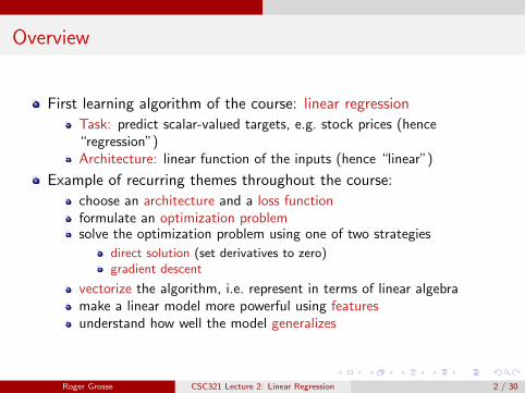
First learning algorithm of the course: linear regression
Task: predict scalar-valued targets, e.g. stock prices (hence“regression”)Architecture: linear function of the inputs (hence “linear”)
Example of recurring themes throughout the course:
choose an architecture and a loss functionformulate an optimization problemsolve the optimization problem using one of two strategies
direct solution (set derivatives to zero)gradient descent
vectorize the algorithm, i.e. represent in terms of linear algebramake a linear model more powerful using featuresunderstand how well the model generalizes
Roger Grosse CSC321 Lecture 2: Linear Regression 2 / 30
Overview
First learning algorithm of the course: linear regression
Task: predict scalar-valued targets, e.g. stock prices (hence“regression”)Architecture: linear function of the inputs (hence “linear”)
Example of recurring themes throughout the course:
choose an architecture and a loss functionformulate an optimization problemsolve the optimization problem using one of two strategies
direct solution (set derivatives to zero)gradient descent
vectorize the algorithm, i.e. represent in terms of linear algebramake a linear model more powerful using featuresunderstand how well the model generalizes
Roger Grosse CSC321 Lecture 2: Linear Regression 2 / 30
Problem Setup
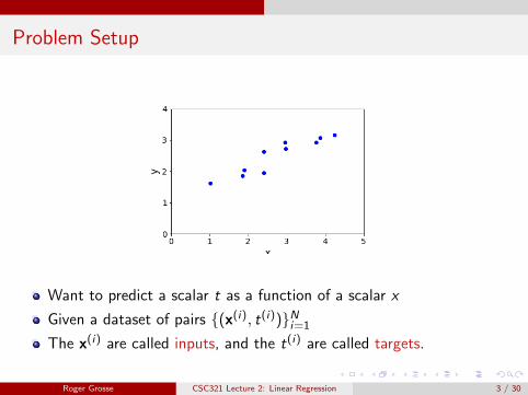
Want to predict a scalar t as a function of a scalar x
Given a dataset of pairs {(x(i), t(i))}Ni=1
The x(i) are called inputs, and the t(i) are called targets.
Roger Grosse CSC321 Lecture 2: Linear Regression 3 / 30
Problem Setup
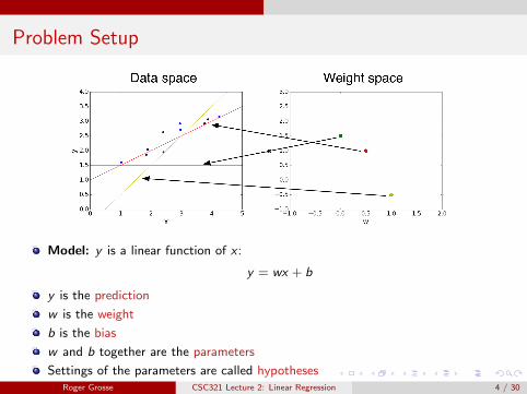
Model: y is a linear function of x :
y = wx + b
y is the prediction
w is the weight
b is the bias
w and b together are the parameters
Settings of the parameters are called hypothesesRoger Grosse CSC321 Lecture 2: Linear Regression 4 / 30
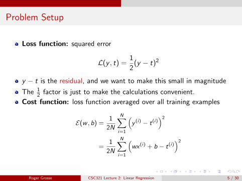
Problem Setup
Loss function: squared error
L(y , t) =1
2(y − t)2
y − t is the residual, and we want to make this small in magnitude
The 12 factor is just to make the calculations convenient.
Cost function: loss function averaged over all training examples
E(w , b) =1
2N
N∑i=1
(y (i) − t(i)
)2=
1
2N
N∑i=1
(wx (i) + b − t(i)
)2
Roger Grosse CSC321 Lecture 2: Linear Regression 5 / 30
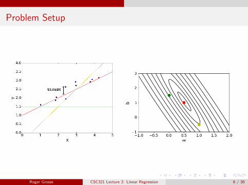
Problem Setup
Roger Grosse CSC321 Lecture 2: Linear Regression 6 / 30
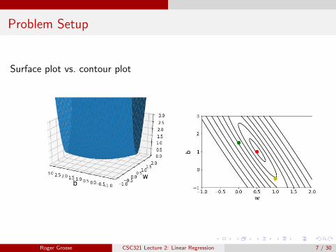
Problem Setup
Surface plot vs. contour plot
Roger Grosse CSC321 Lecture 2: Linear Regression 7 / 30
Problem setup
Suppose we have multiple inputs x1, . . . , xD . This is referred to asmultivariable regression.
This is no different than the single input case, just harder to visualize.
Linear model:y =
∑j
wjxj + b
Roger Grosse CSC321 Lecture 2: Linear Regression 8 / 30
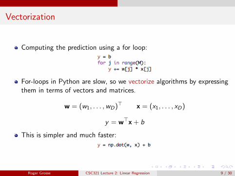
Vectorization
Computing the prediction using a for loop:
For-loops in Python are slow, so we vectorize algorithms by expressingthem in terms of vectors and matrices.
w = (w1, . . . ,wD)> x = (x1, . . . , xD)
y = w>x + b
This is simpler and much faster:
Roger Grosse CSC321 Lecture 2: Linear Regression 9 / 30

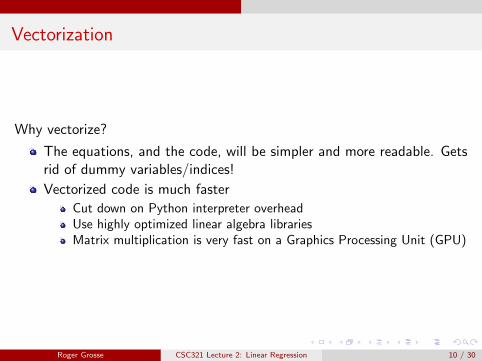
Vectorization
Why vectorize?
The equations, and the code, will be simpler and more readable. Getsrid of dummy variables/indices!
Vectorized code is much faster
Cut down on Python interpreter overheadUse highly optimized linear algebra librariesMatrix multiplication is very fast on a Graphics Processing Unit (GPU)
Roger Grosse CSC321 Lecture 2: Linear Regression 10 / 30
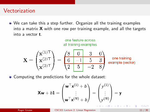
Vectorization
We can take this a step further. Organize all the training examplesinto a matrix X with one row per training example, and all the targetsinto a vector t.
Computing the predictions for the whole dataset:
Xw + b1 =
w>x(1) + b...
w>x(N) + b
=
y (1)
...
y (N)
= y
Roger Grosse CSC321 Lecture 2: Linear Regression 11 / 30
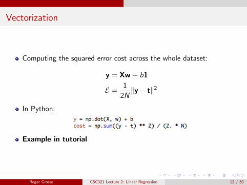
Vectorization
Computing the squared error cost across the whole dataset:
y = Xw + b1
E =1
2N‖y − t‖2
In Python:
Example in tutorial
Roger Grosse CSC321 Lecture 2: Linear Regression 12 / 30
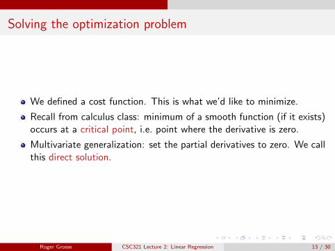
Solving the optimization problem
We defined a cost function. This is what we’d like to minimize.
Recall from calculus class: minimum of a smooth function (if it exists)occurs at a critical point, i.e. point where the derivative is zero.
Multivariate generalization: set the partial derivatives to zero. We callthis direct solution.
Roger Grosse CSC321 Lecture 2: Linear Regression 13 / 30
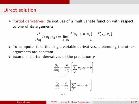
Direct solution
Partial derivatives: derivatives of a multivariate function with respectto one of its arguments.
∂
∂x1f (x1, x2) = lim
h→0
f (x1 + h, x2)− f (x1, x2)
h
To compute, take the single variable derivatives, pretending the otherarguments are constant.Example: partial derivatives of the prediction y
∂y
∂wj=
∂
∂wj
∑j′
wj′xj′ + b
= xj
∂y
∂b=
∂
∂b
∑j′
wj′xj′ + b
= 1
Roger Grosse CSC321 Lecture 2: Linear Regression 14 / 30
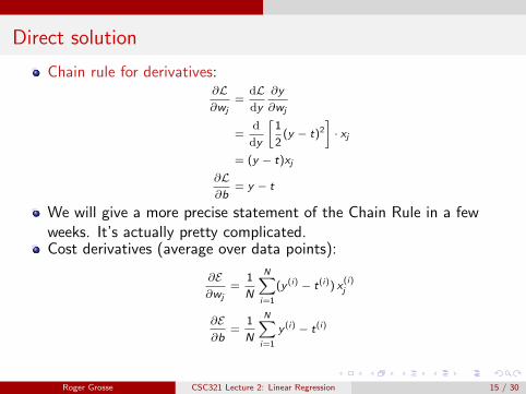
Direct solution
Chain rule for derivatives:∂L∂wj
=dLdy
∂y
∂wj
=d
dy
[1
2(y − t)2
]· xj
= (y − t)xj
∂L∂b
= y − t
We will give a more precise statement of the Chain Rule in a fewweeks. It’s actually pretty complicated.Cost derivatives (average over data points):
∂E∂wj
=1
N
N∑i=1
(y (i) − t(i)) x(i)j
∂E∂b
=1
N
N∑i=1
y (i) − t(i)
Roger Grosse CSC321 Lecture 2: Linear Regression 15 / 30
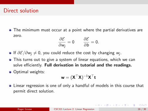
Direct solution
The minimum must occur at a point where the partial derivatives arezero.
∂E∂wj
= 0∂E∂b
= 0.
If ∂E/∂wj 6= 0, you could reduce the cost by changing wj .
This turns out to give a system of linear equations, which we cansolve efficiently. Full derivation in tutorial and the readings.
Optimal weights:w = (X>X)−1X>t
Linear regression is one of only a handful of models in this course thatpermit direct solution.
Roger Grosse CSC321 Lecture 2: Linear Regression 16 / 30
Gradient Descent
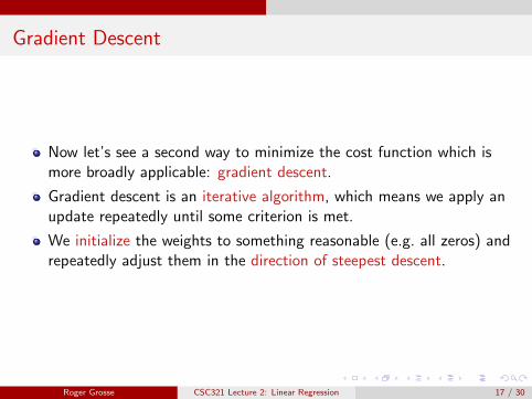
Now let’s see a second way to minimize the cost function which ismore broadly applicable: gradient descent.
Gradient descent is an iterative algorithm, which means we apply anupdate repeatedly until some criterion is met.
We initialize the weights to something reasonable (e.g. all zeros) andrepeatedly adjust them in the direction of steepest descent.
Roger Grosse CSC321 Lecture 2: Linear Regression 17 / 30
Gradient descent
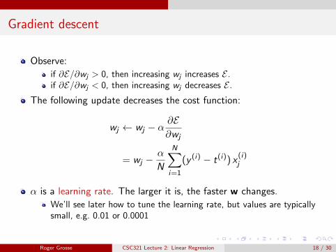
Observe:
if ∂E/∂wj > 0, then increasing wj increases E .if ∂E/∂wj < 0, then increasing wj decreases E .
The following update decreases the cost function:
wj ← wj − α∂E∂wj
= wj −α
N
N∑i=1
(y (i) − t(i)) x(i)j
α is a learning rate. The larger it is, the faster w changes.
We’ll see later how to tune the learning rate, but values are typicallysmall, e.g. 0.01 or 0.0001
Roger Grosse CSC321 Lecture 2: Linear Regression 18 / 30
Gradient descent
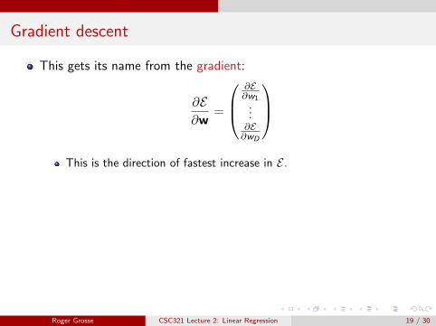
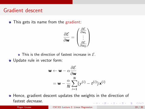
This gets its name from the gradient:
∂E∂w
=
∂E∂w1
...∂E∂wD
This is the direction of fastest increase in E .
Update rule in vector form:
w← w − α ∂E∂w
= w − α
N
N∑i=1
(y (i) − t(i)) x(i)
Hence, gradient descent updates the weights in the direction offastest decrease.
Roger Grosse CSC321 Lecture 2: Linear Regression 19 / 30
Gradient descent
Visualization:http://www.cs.toronto.edu/~guerzhoy/321/lec/W01/linear_
regression.pdf#page=21
Roger Grosse CSC321 Lecture 2: Linear Regression 20 / 30
Gradient descent
Why gradient descent, if we can find the optimum directly?
GD can be applied to a much broader set of modelsGD can be easier to implement than direct solutions, especially withautomatic differentiation softwareFor regression in high-dimensional spaces, GD is more efficient thandirect solution (matrix inversion is an O(D3) algorithm).
Roger Grosse CSC321 Lecture 2: Linear Regression 21 / 30
Feature mappings
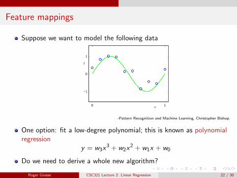
Suppose we want to model the following data
x
t
0 1
−1
0
1
-Pattern Recognition and Machine Learning, Christopher Bishop.
One option: fit a low-degree polynomial; this is known as polynomialregression
y = w3x3 + w2x
2 + w1x + w0
Do we need to derive a whole new algorithm?
Roger Grosse CSC321 Lecture 2: Linear Regression 22 / 30
Feature mappings
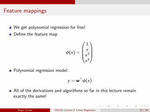
We get polynomial regression for free!
Define the feature map
φ(x) =
1xx2
x3
Polynomial regression model:
y = w>φ(x)
All of the derivations and algorithms so far in this lecture remainexactly the same!
Roger Grosse CSC321 Lecture 2: Linear Regression 23 / 30

Fitting polynomials
y = w0
x
t
M = 0
0 1
−1
0
1
-Pattern Recognition and Machine Learning, Christopher Bishop.
Roger Grosse CSC321 Lecture 2: Linear Regression 24 / 30
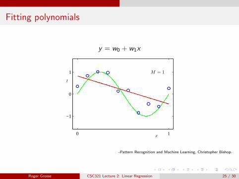
Fitting polynomials
y = w0 + w1x
x
t
M = 1
0 1
−1
0
1
-Pattern Recognition and Machine Learning, Christopher Bishop.
Roger Grosse CSC321 Lecture 2: Linear Regression 25 / 30
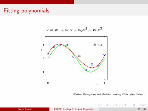
Fitting polynomials
y = w0 + w1x + w2x2 + w3x
3
x
t
M = 3
0 1
−1
0
1
-Pattern Recognition and Machine Learning, Christopher Bishop.
Roger Grosse CSC321 Lecture 2: Linear Regression 26 / 30
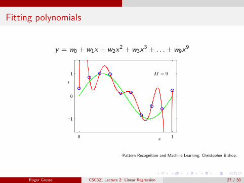
Fitting polynomials
y = w0 + w1x + w2x2 + w3x
3 + . . .+ w9x9
x
t
M = 9
0 1
−1
0
1
-Pattern Recognition and Machine Learning, Christopher Bishop.
Roger Grosse CSC321 Lecture 2: Linear Regression 27 / 30
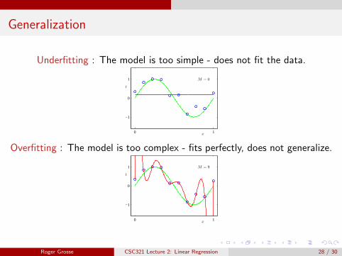
Generalization
Underfitting : The model is too simple - does not fit the data.
x
t
M = 0
0 1
−1
0
1
Overfitting : The model is too complex - fits perfectly, does not generalize.
x
t
M = 9
0 1
−1
0
1
Roger Grosse CSC321 Lecture 2: Linear Regression 28 / 30
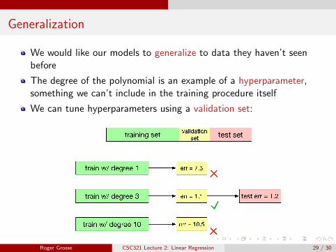
Generalization
We would like our models to generalize to data they haven’t seenbefore
The degree of the polynomial is an example of a hyperparameter,something we can’t include in the training procedure itself
We can tune hyperparameters using a validation set:
Roger Grosse CSC321 Lecture 2: Linear Regression 29 / 30
Foreshadowing
Feature maps aren’t a silver bullet:
It’s not always easy to pick good features.In high dimensions, polynomial expansions can get very large!
Until the last few years, a large fraction of the effort of building agood machine learning system was feature engineering
We’ll see that neural networks are able to learn nonlinear functionsdirectly, avoiding hand-engineering of features
Roger Grosse CSC321 Lecture 2: Linear Regression 30 / 30