Embed Size (px)
DESCRIPTION
CSE 554 Lecture 8: Alignment. Fall 2014. Review. Fairing (smoothing) Relocating vertices to achieve a smoother appearance Method: centroid averaging Simplification Reducing vertex count Method: edge collapsing. Registration. Fitting one model to match the shape of another. Registration. - PowerPoint PPT Presentation
Citation preview

CSE554 Alignment Slide 1
CSE 554
Lecture 8: Alignment
CSE 554
Lecture 8: Alignment
Fall 2015
CSE554 Alignment Slide 2
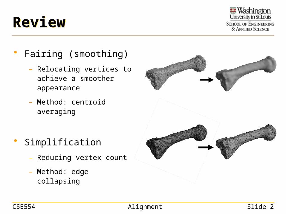
ReviewReview
• Fairing (smoothing)
– Relocating vertices to achieve a smoother appearance
– Method: centroid averaging
• Simplification
– Reducing vertex count
– Method: edge collapsing

CSE554 Alignment Slide 3
RegistrationRegistration
• Fitting one model to match the shape of another

CSE554 Alignment Slide 4
RegistrationRegistration
• Applications
– Tracking and motion analysis
– Automated annotation

CSE554 Alignment Slide 5
RegistrationRegistration
• Challenges: global and local shape differences
– Imaging causes global shifts and tilts
• Requires alignment
– The shape of the organ or tissue differs in subjects and evolve over time
• Requires deformation
Brain outlines of two mice After alignment After deformation

CSE554 Alignment Slide 6
AlignmentAlignment
• Registration by translation or rotation
– The structure stays “rigid” under these two transformations
• Called rigid-body or isometric (distance-preserving) transformations
– Mathematically, they are represented as matrix/vector operations
Before alignment After alignment

CSE554 Alignment Slide 7
Transformation Math Transformation Math
• Translation
– Vector addition:
– 2D:
– 3D:
px'
py' vx
vy px
py
px'
py'
pz'
vxvyvz
pxpypz
p' v p
p
p'
v

CSE554 Alignment Slide 8
Transformation Math Transformation Math
• Rotation
– Matrix product:
– 2D:
• Rotate around the origin!
• To rotate around another point q:
px'
py' R px
py
R Cos SinSin Cos
p' R p
p
p'
x
y
p' R p q q p
p'
x
y
q

CSE554 Alignment Slide 9
Transformation Math Transformation Math
• Rotation
– Matrix product:
– 3D:
px'
py'
pz'
R pxpypz
Around X axis:
Around Y axis:
Around Z axis:
p' R p
x
y
z
Rx 1 0 00 Cos Sin0 Sin Cos
Ry Cosa 0 Sina
0 1 0Sina 0 Cosa
Rz Cosa Sina 0Sina Cosa 0
0 0 1
Any arbitrary 3D rotation can be composed from these three rotations

CSE554 Alignment Slide 10
Transformation Math Transformation Math
• Properties of an arbitrary rotational matrix
– Orthonormal (orthogonal and normal):
• Examples:
– Easy to invert:
R RT I
Cos SinSin Cos Cos Sin
Sin Cos 1 00 1
1 0 00 Cos Sin0 Sin Cos
1 0 00 Cos Sin0 Sin Cos
1 0 00 1 00 0 1
R1 RT

CSE554 Alignment Slide 11
Transformation Math Transformation Math
• Properties of an arbitrary rotational matrix
– Any orthonormal 3x3 matrix represents a rotation around some axis (not limited to X,Y,Z)
• The angle of rotation can be calculated from the trace of the matrix
– Trace: sum of diagonal entries
– 2D: The trace equals 2 Cos(a), where a is the rotation angle
– 3D: The trace equals 1 + 2 Cos(a)
• The larger the trace, the smaller the rotation angle
Cos SinSin Cos Cos Sin
Sin Cos 1 00 1
1 0 00 Cos Sin 0 Sin Cos
1 0 00 Cos Sin 0 Sin Cos
1 0 00 1 00 0 1
Examples:

CSE554 Alignment Slide 12
AlignmentAlignment
• Input: two models represented as point sets
– Source and target
• Output: locations of the translated and rotated source points
Source
Target

CSE554 Alignment Slide 13
AlignmentAlignment
• Method 1: Principal component analysis (PCA)
– Aligning principal directions
• Method 2: Singular value decomposition (SVD)
– Optimal alignment given prior knowledge of correspondence
• Method 3: Iterative closest point (ICP)
– An iterative SVD algorithm that computes correspondences as it goes

CSE554 Alignment Slide 14
Method 1: PCAMethod 1: PCA
• Compute a shape-aware coordinate system for each model
– Origin: Centroid of all points
– Axes: Directions in which the model varies most or least
• Transform the source to align its origin/axes with the target

CSE554 Alignment Slide 15
Basic Math Basic Math
• Eigenvectors and eigenvalues
– Let M be a square m-by-m matrix, v is an eigenvector and λ is an eigenvalue if:
– Any scalar multiples of an eigenvector is also an eigenvector (with the same eigenvalue).
• So an eigenvector should be treated as a “line”, rather than a vector
– There are at most m non-zero eigenvectors
• If M is symmetric, its eigenvectors are pairwise orthogonal
M v v

CSE554 Alignment Slide 16
Method 1: PCAMethod 1: PCA
• Computing axes: Principal Component Analysis (PCA)
– Consider a set of points p1,…,pn with centroid location c
• Construct matrix P whose i-th column is vector pi – c
– 2D (2 by n):
– 3D (3 by n):
• Build the covariance matrix:
– 2D: a 2 by 2 matrix
– 3D: a 3 by 3 matrix
– Symmetric!
M P PT
pi
c
P p1x cx p2x cx ... pnx cxp1y cy p2y cy ... pny cy
P
p1x cx p2x cx ... pnx cxp1y cy p2y cy ... pny cyp1z cz p2z cz ... pnz cz

CSE554 Alignment Slide 17
Method 1: PCAMethod 1: PCA
• Computing axes: Principal Component Analysis (PCA)
– Eigenvectors of the covariance matrix represent principal directions of shape variation (2 in 2D; 3 in 3D)
– Eigenvalues indicate amount of variation along each eigenvector
• Eigenvector with largest (smallest) eigenvalue is the direction where the model shape varies the most (least)
Eigenvector with the larger eigenvalue
Eigenvector with the smaller eigenvalue

CSE554 Alignment Slide 18
Method 1: PCAMethod 1: PCA
• PCA-based alignment
– Let cS,cT be centroids of source and target.
– First, translate source to align cS with cT:
– Next, find rotation R that aligns two sets of PCA axes, and rotate source around cT:
– Combined:
pi pi cT cS
pi' cT R pi cTpi' cT R pi cS
pi
pi
pi'
cT
cS
cT
cT

CSE554 Alignment Slide 19
Method 1: PCAMethod 1: PCA
• Oriented axes
– 2D: Y is ccw from X
– 3D: X,Y,Z follow right-handed rule X
Y
X
Y
Z

CSE554 Alignment Slide 20
Method 1: PCAMethod 1: PCA
• Finding rotation between two sets of oriented axes
– Let A, B be two matrices whose columns are the axes
• The axes are orthogonal and normalized (i.e., both A and B are orthonormal)
– We wish to compute a rotation matrix R such that:
– Notice that A and B are orthonormal, so we have:
R A B
R B A1 B AT
A
3
2 1
2
1
2
3
2
B 1 00 1
R
3
2
1
2
12
3
2
30o
X1X2
Y1 Y2
X1 Y1X2 Y2

CSE554 Alignment Slide 21
Method 1: PCAMethod 1: PCA
• How to get oriented axes from eigenvectors?
– In 2D, two eigenvectors can define 2 sets of oriented axes (whose X,Y correspond to 1st and 2nd eigenvectors)
1st eigenvector 2nd eigenvector
X
Y
X
Y

CSE554 Alignment Slide 22
Method 1: PCAMethod 1: PCA
• How to get oriented axes from eigenvectors?
– In 3D, three eigenvectors can define 4 sets of oriented axes (whose X,Y,Z correspond to 1st, 2nd, 3rd eigenvectors)
1st eigenvector 2nd eigenvector 3rd eigenvector
X
X
X
X
Y
Y
Y
Y
Z
Z
Z
Z

CSE554 Alignment Slide 23
Method 1: PCAMethod 1: PCA
• Finding rotation between two sets of eigenvectors
– Fix the orientation of the target axes.
– For each possible orientation of the source axes, compute R
– Pick the R with smallest rotation angle (by checking the trace of R)
• Assuming the source is “close” to the target!
Smaller rotation Larger rotation

CSE554 Alignment Slide 24
Method 1: PCAMethod 1: PCA
• Limitations
– Axes can be unreliable for circular objects
• Eigenvalues become similar, and eigenvectors become unstable
Rotation by a small angle PCA result

CSE554 Alignment Slide 25
Method 1: PCAMethod 1: PCA
• Limitations
– Centroid and axes are affected by noise
Noise
Axes are affected PCA result

CSE554 Alignment Slide 26
Method 2: SVDMethod 2: SVD
• Optimal alignment between corresponding points
– Assuming that for each source point, we know where the corresponding target point is.

CSE554 Alignment Slide 27
Method 2: SVDMethod 2: SVD
• Formulating the problem
– Source points p1,…,pn with centroid location cS
– Target points q1,…,qn with centroid location cT
• qi is the corresponding point of pi
– After centroid alignment and rotation by some R, a transformed source point is located at:
– We wish to find the R that minimizes sum of pair-wise distances:
pi' cT R pi cSE
i1
n qi pi'2

CSE554 Alignment Slide 28
Method 2: SVDMethod 2: SVD
• An equivalent formulation
– Let P be a matrix whose i-th column is vector pi – cS
– Let Q be a matrix whose i-th column is vector qi – cT
– Consider the cross-covariance matrix:
– Find the orthonormal matrix R that maximizes the trace:
M P QT
TrR M

CSE554 Alignment Slide 29
Method 2: SVDMethod 2: SVD
• Solving the minimization problem
– Singular value decomposition (SVD) of an m by m matrix M:
• U,V are m by m orthonormal matrices (i.e., rotations)
• W is a diagonal m by m matrix with non-negative entries
– The orthonormal matrix (rotation) is the R that maximizes the trace
– SVD is available in Mathematica and many Java/C++ libraries
TrR MM U W VT
R V UT

CSE554 Alignment Slide 30
Method 2: SVDMethod 2: SVD
• SVD-based alignment: summary
– Forming the cross-covariance matrix
– Computing SVD
– The optimal rotation matrix is
– Translate and rotate the source:
M P QT
M U W VT
R V UT
pi' cT R pi cSTranslate
Rotate

CSE554 Alignment Slide 31
Method 2: SVDMethod 2: SVD
• Advantage over PCA: more stable
– As long as the correspondences are correct

CSE554 Alignment Slide 32
Method 2: SVDMethod 2: SVD
• Advantage over PCA: more stable
– As long as the correspondences are correct

CSE554 Alignment Slide 33
Method 2: SVDMethod 2: SVD
• Limitation: requires accurate correspondences
– Which are usually not available

CSE554 Alignment Slide 34
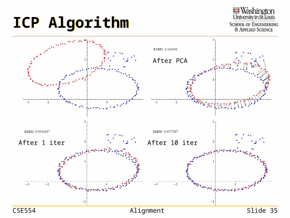
Method 3: ICPMethod 3: ICP
• Iterative closest point (ICP)
– Use PCA alignment to obtain an initial alignment
– Alternate between finding correspondences and aligning the corresponding points
• For each transformed source point, assign the closest target point as its corresponding point.
• Align source and target by SVD.
• Repeat until a termination criteria is met.
CSE554 Alignment Slide 35
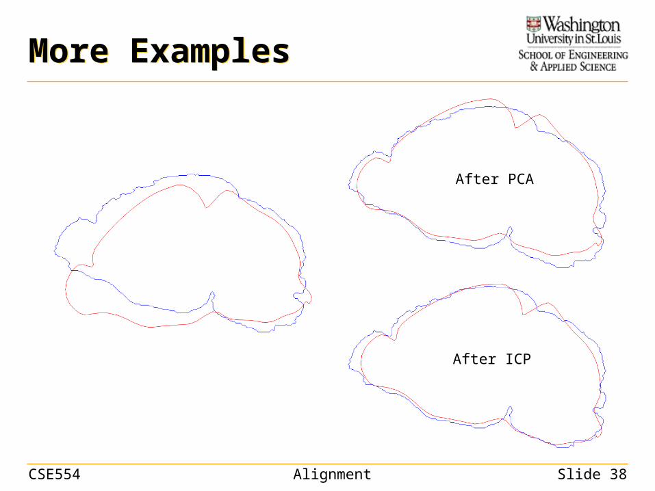
ICP AlgorithmICP Algorithm
After PCA
After 10 iterAfter 1 iter

CSE554 Alignment Slide 36
ICP AlgorithmICP Algorithm
After PCA
After 10 iterAfter 1 iter

CSE554 Alignment Slide 37
ICP AlgorithmICP Algorithm
• Termination criteria
– A user-given maximum iteration is reached
– The improvement of fitting is small
• Root Mean Squared Distance (RMSD):
– Captures average deviation in all corresponding pairs
• Stops the iteration if the difference in RMSD before and after each iteration falls beneath a user-given threshold
i1n qi pi'2
n