CSE 573: Artificial Intelligence

Winter 2019

A* Search

Hanna Hajishirzi Based on slides from Luke Zettlemoyer, Dan Klein

Multiple slides from Stuart Russell or Andrew Moore

Announcements

! PS1 is due on Friday ! Discussion board is up and running

!2

Recap

! Rational Agents ! Problem state spaces and search

problems ! Uninformed search algorithms

! DFS ! BFS ! UCS

! Heuristics ! Best First Greedy

!3

Example: Pancake Problem

Cost: Number of pancakes flipped

Action: Flip over the top n pancakes

Example: Pancake Problem

Example: Pancake Problem

3

2

4

3

3

2

2

2

4

State space graph with costs as weights

34

3

4

2

3

General Tree Search

Action: flip top two

Cost: 2

Action: flip all fourCost: 4

Path to reach goal: Flip four, flip three

Total cost: 7

Uniform Cost Search

! Strategy: expand lowest path cost

! The good: UCS is complete and optimal!

! The bad: ! Explores options in every

“direction” ! No information about goal

location Start Goal

…

c ≤ 3

c ≤ 2

c ≤ 1

Example: Heuristic Function

h(x): assigns a value to a state

Example: Heuristic FunctionHeuristic: the largest pancake that is still out of place

43

0

2

3

3

3

4

4

3

4

4

4

h(x)

Best First (Greedy)

! Strategy: expand a node that you think is closest to a goal state ! Heuristic: estimate of

distance to nearest goal for each state

! A common case: ! Best-first takes you

straight to the (wrong) goal

! Worst-case: like a wrongly-guided DFS

…b

…b

Combining UCS and Greedy

! A* Search orders by the sum: f(n) = g(n) + h(n)

S a d

b

h=5

h=6

h=2

1

5

11

2

h=6

h=0

ch=7

3

e h=11

Example: Teg Grenager

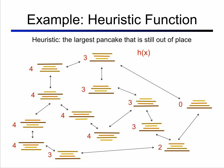
! Uniform-cost orders by path cost, or backward cost f(n)=g(n)! Best-first orders by goal proximity, or forward cost f(n)=h(n)

1

Combining#UCS#and#Greedy#

!  UniformKcost#orders#by#path#cost,#or#backward-cost--g(n)#!  Greedy#orders#by#goal#proximity,#or#forward-cost--h(n)-

!  A*#Search#orders#by#the#sum:#f(n)#=#g(n)#+#h(n)-

S a d

b

G h=5

h=6

h=2

1

8

1 1

2

h=6 h=0 c

h=7

3

e h=1 1

Example:#Teg#Grenager#

S

a

b

c

e d

d G

G

g = 0 h=6

g = 1 h=5

g = 2 h=6

g = 3 h=7

g = 4 h=2

g = 6 h=0

g = 9 h=1

g = 10 h=2

g = 12 h=0

G

! Should we stop when we enqueue a goal?

When should A* terminate?

S

B

A

G

2

3

2

2h = 1

h = 2

h = 0

h = 3

! No: only stop when we dequeue a goal

Is A* Optimal?

A

GS

13

h = 6

h = 0

5

h = 7

! What went wrong? ! Actual bad goal cost < estimated good goal cost ! We need estimates to be less than actual costs!

Admissible Heuristics

! A heuristic h is admissible (optimistic) if:

where is the true cost to a nearest goal

4 15

! Examples:

! Coming up with admissible heuristics is most of what’s involved in using A* in practice.

Optimality of A*

…Assume: ! G* is an optimal goal

! G is a sub-optimal goal

! h is admissible

Claim: ! G* will exit fringe before G

Optimality of A*: Blocking

…Notation: ! g(n) = cost to node n

! h(n) = estimated cost from n

to the nearest goal (heuristic)

! f(n) = g(n) + h(n) =estimated total cost via n

! G*: a lowest cost goal node

! G: another goal node

Optimality of A*: Blocking

Proof: ! What could go wrong? ! We’d have to have to pop a

suboptimal goal G off the fringe before G*

…

! This can’t happen: ! For all nodes n on the

best path to G* ! f(n) < f(G)

! So, G* will be popped before G

Properties of A*

…b

…b

Uniform-Cost A*

UCS vs A* Contours

! Uniform-cost expanded in all directions

! A* expands mainly toward the goal, but does hedge its bets to ensure optimality

Start Goal

Start Goal

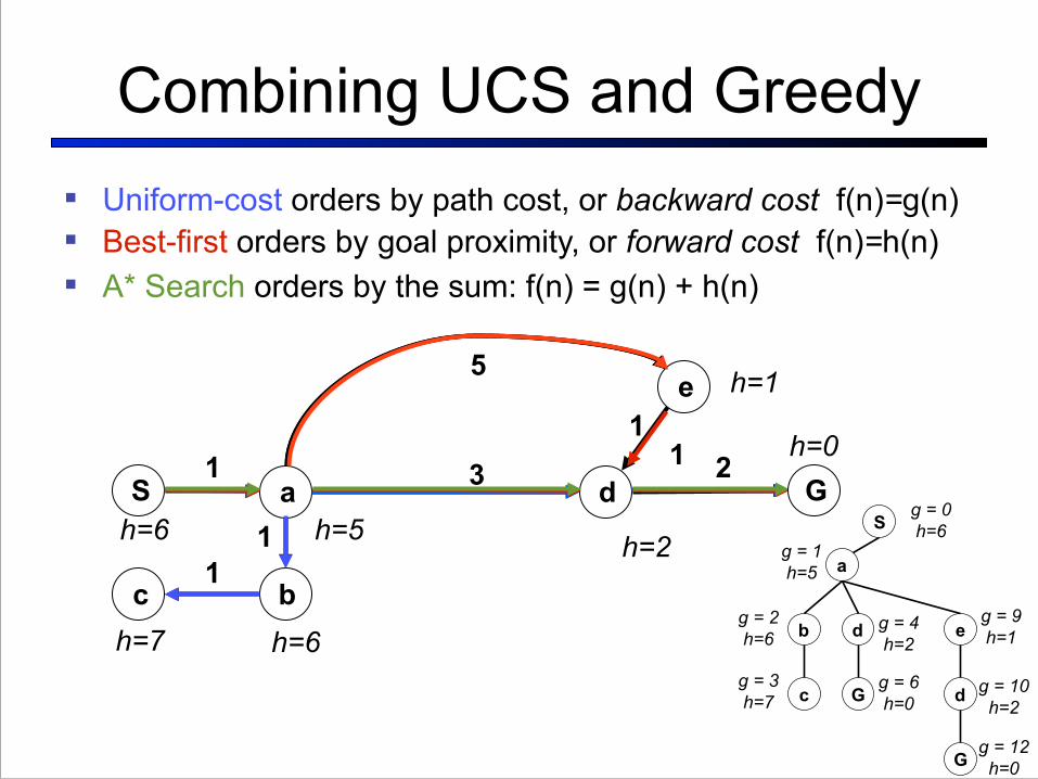
UCS! 900 States

!21

Astar! 180 States

!22

Recent Literature

! Joint A* CCG Parsing and Semantic Role Labeling [EMNLP’15]

! Diagram parsing [ECCV’16]

!23

Lexical Category Choicexi !NP | S\NP | (S\NP)/PP | . . .

One dependency is created for every argument of the categoryS\NP ! S\NP

(S\NP)/PP ! (S\NP)/PP, (S\NP)/PP

. . .Preposition choice for PP arguments(S\NP)/PP ! (S\NP)/PP

in | (S\NP)/PP

for | . . .

. . .Semantic role label choice for the argumentS\NP ! S\NP

ARG0

| S\NP

ARG1

| . . .

(S\NP)/PP ! (S\NP

ARG0

)/PP | (S\NP

ARG1

)/PP . . .(S\NP)/PP

X ! (S\NP)/PP

X

ARG0

| (S\NP)/PP

X

ARG1

. . .

. . .Attachment choiceARG0 ! x0 | . . . | xi�1 | xi+1 | . . . | xN

ARG1 ! x0 | . . . | xi�1 | xi+1 | . . . | xN

. . .

(a) The grammar GENLEX (x

i

)

confirm

S\NP (S\NP)/NP

NP

S\NP (S\NP)/NP (S\NP)/NP

ARG0 ARG1

?

He reports refused

(b) Visualization of a fragment of GENLEX (confirm)

Figure 4: (a) The grammar GENLEX (x

i

), which defines the space of extended lexical entries,and (b) a visualization of a fragment of GENLEX (confirm). Extended lexical entries, includingconfirm `(S\NP

ARG0=he

)/NP

ARG1=reports

and confirm `NP , are specified by choosing one cate-gory (top level in both a and b), enumerating all arguments (second level), selecting the preposition forPP arguments (when present), selecting a semantic role label for each, and finally choosing the argumenthead word. The features are local to the grammar rules, enabling efficient dynamic programs for upperbound computations on partially specified entries, such as confirm `(S\NP

r=a

)/NP

ARG1=reports

.

then create an upper bound for the parse as a sumof upper bounds for words. The bound is not exact,because the grammar may not allow the combina-tion of the best lexical entry for each word.

Section 5.1 gives a declarative definition of h

for any partial parse, and 5.2 explains how to effi-ciently compute h during parsing.

5.1 Upper Bounds for Partial Parses

This section defines the upper bound on the Viterbioutside score h(yi,j) for any partial parse yi,j ofspan i . . . j. For example, in the parse in Figure3, y3,5 is the partial parse of confirm or deny withcategory (S\NP)/NP .

As explained in Section 4, a parse can be de-composed into a series of extended lexical entries.Similarly, a partial parse can be viewed as a se-ries of partially specified extended lexical entriesy0 . . . yN . For example, in Figure 3, the partialparse of the span confirm or deny reports, the ex-tended lexical entries for the words outside thespan (He, refused and to) are completely unspeci-fied. The extended lexical entries for words insidethe span have specified categories, but can containunderspecified dependencies:

confirm ` (S\NP

r=a

)/NP

ARG1=reports

or ` conj

deny ` (S\NP

r

0=a

0)/NP

ARG1=reports

reports ` NP

Therefore, we can compute an upper bound for

the outside score of a partial parse as a sum ofthe upper bounds of the unspecified components ofeach extended lexical entry. Note that because thederivation features are constrained to be 0, theydo not affect the calculation of the upper bound.

We can then find an upper bound for completelyunspecified spans using by summing the upperbounds for the words. We can pre-compute an up-per bound for the span hi,j for every span i, j as:

hi,j =

jX

k=i

max

yk

2GENLEX (xk

)✓ · �(x, yk)

The max can be efficiently computed using theViterbi algorithm on GENLEX (xk) (as describedin Section 4).

The upper bound on the outside score of a par-tial parse is then the sum of the upper bounds ofthe words outside the parse, and the sum of thescores of the best possible specifications for eachunderspecified dependency:

h(yi,j) =

X

hf,c,n,?,?,?i2deps(yi,j

)

max

a0,p0,r0✓ · �(hf, c, n, p

0, a

0, r

0i)

+ h0,i�1 + hj+1,N

where deps(y) returns the underspecified depen-dencies from partial parse.

For example, in Figure 3, the upper bound forthe outside score of the partial parse of confirmor deny reports is the sum of the upper bounds

1448

A Diagram Is Worth A Dozen Images 9

Arrowheads

Arrows

Text

Blobs

InterobjectLinkage

Tree

IntraobjectLinkage

SectionTitle

FoodWebImageTitle

IntraobjectLabel

Tree

FoodWeb

Fromtheabovefoodwebdiagram,whatwillleadtoanincreaseinthepopulationofdeer?a)increaseinlionb)decreaseinplantsc)decreaseinliond)increaseinpikaMultipleChoiceQuestion:

Fig. 4. An image from the AI2D dataset showing some of its rich annotations and amultiple choice question.

15000 multiple choice questions associated to the diagrams. We divide the AI2D

dataset into a train set with 4000 images and a blind test set with 1000 imagesand report our numbers on this blind test set.

The images are collected by scraping Google Image Search with seed termsderived from the chapter titles in Grade 1 - 6 science textbooks. Each image isannotated using Amazon Mechanical Turk (AMT). Annotating each image withrich annotations such as ours, is a rather complicated task and must be brokendown into several phases to maximize the level of agreement obtained from turk-ers. Also, these phases need to be carried out sequentially to avoid conflicts in theannotations. The phases involve (1) annotating the four low-level constituents,(2) categorizing the text boxes into one of four categories: relationship with thecanvas, relationship with a diagrammatic element, intra-object relationship andinter-object relationship, (3) categorizing the arrows into one of three categories:intra-object relationship, inter-object relationship or neither, (4) labelling intra-object linkage and inter-object linkage relationships. For this step, we displayarrows to turkers and have them choose the origin and destination constituentsin the diagram, (5) labelling intra-object label, intra-object region label and ar-row descriptor relationships. For this purpose, we display text boxes to turkersand have them choose the constituents related to it, and finally (6) multiplechoice questions with answers, representing grade school science questions arethen obtained for each image using AMT. Figure 4 shows some of the rich an-notations obtained for an image in the dataset along with one of its associatedmultiple choice questions.

Creating Heuristics

! What are the states? ! How many states? ! What are the actions? ! What states can I reach from the start state? ! What should the costs be?

8-puzzle:

8 Puzzle I

! Heuristic: Number of tiles misplaced

! h(start) = 8

Average nodes expanded when optimal path has length…

…4 steps …8 steps …12 steps

UCS 112 6,300 3.6 x 106

TILES 13 39 227

! Is it admissible?

8 Puzzle II

! What if we had an easier 8-puzzle where any tile could slide any direction at any time, ignoring other tiles?

! Total Manhattan distance

! h(start) =3 + 1 + 2 + …

= 18

Average nodes expanded when optimal path has length…

…4 steps …8 steps …12 steps

TILES 13 39 227MANHATTAN 12 25 73! Admissible?

8 Puzzle III

! How about using the actual cost as a heuristic? ! Would it be admissible? ! Would we save on nodes expanded? ! What’s wrong with it?

! With A*: a trade-off between quality of estimate and work per node!

In fact,

! Coming up with good heuristics is important in AI ! Distinguishes between AI and Theory CS ! Add intuitions on how to solve NP-hard/

intractable problems

!28

Creating Admissible Heuristics! Most of the work in solving hard search problems

optimally is in coming up with admissible heuristics

! Often, admissible heuristics are solutions to relaxed problems, where new actions are available

15366

! Inadmissible heuristics are often useful too (why?)

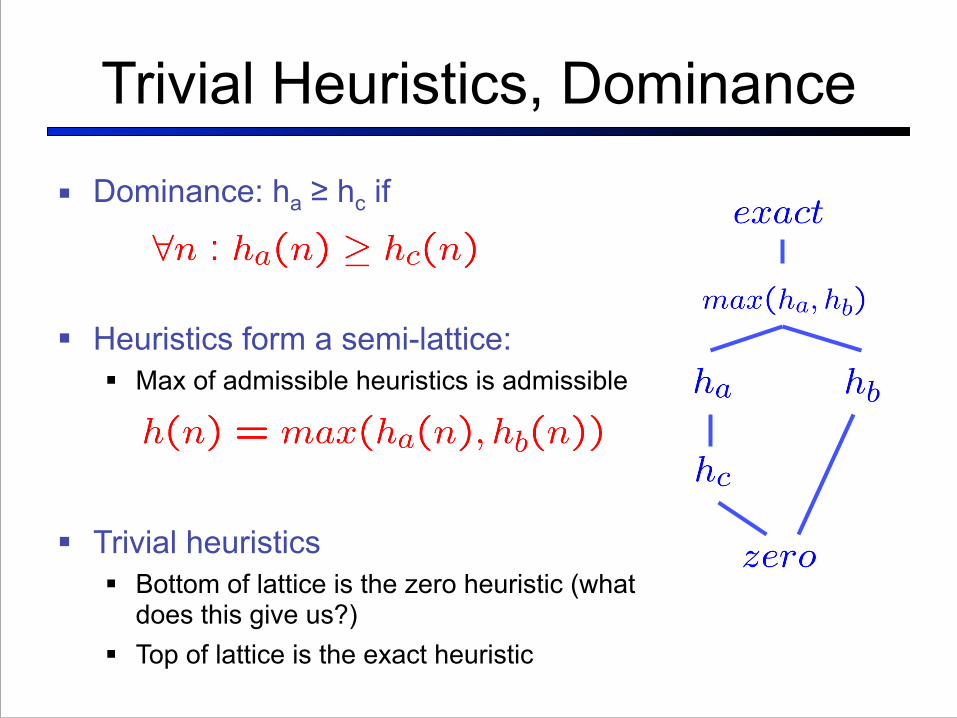
Trivial Heuristics, Dominance

! Dominance: ha ≥ hc if

! Heuristics form a semi-lattice: ! Max of admissible heuristics is admissible

! Trivial heuristics ! Bottom of lattice is the zero heuristic (what

does this give us?) ! Top of lattice is the exact heuristic

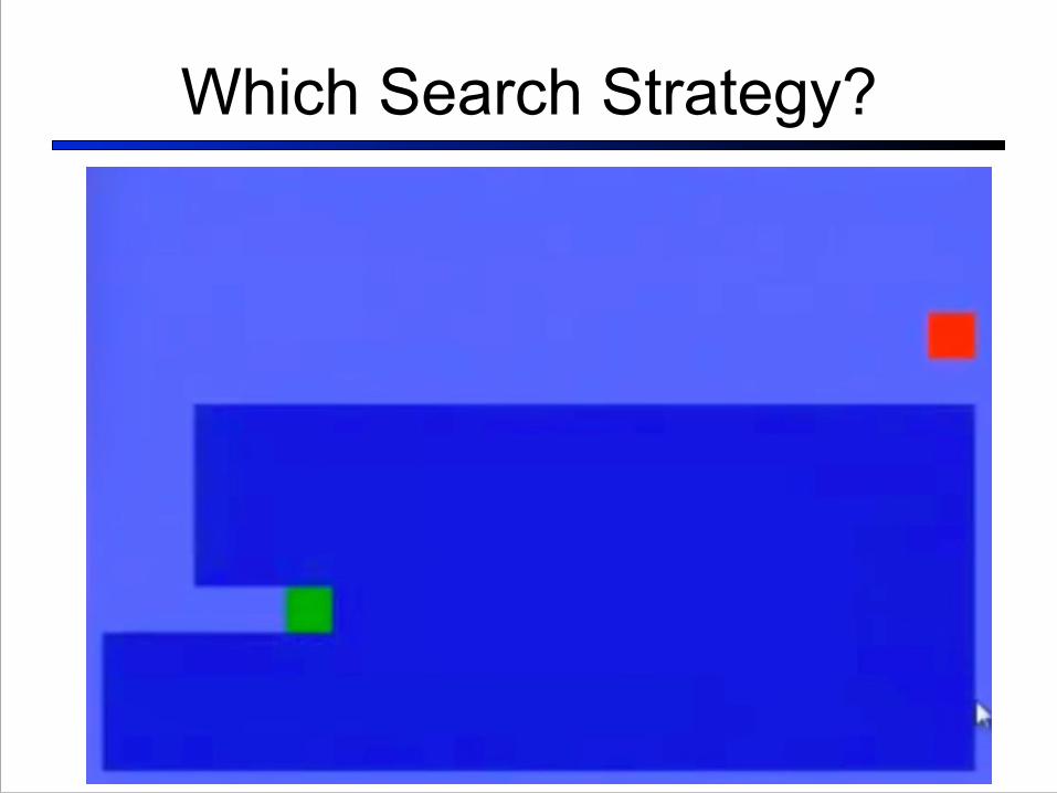
Which Search Strategy?

!31

Which Search Strategy?

!32

Which Search Strategy?

!33

Which Search Strategy?

!34

Which Search Strategy?

!35

Tree Search: Extra Work!

! Failure to detect repeated states can cause exponentially more work. Why?

Graph Search

! In BFS, for example, we shouldn’t bother expanding some nodes (which, and why?)

S

a

b

d p

a

c

e

p

h

f

r

q

q c G

a

qe

p

h

f

r

q

q c G

a

Graph Search! Idea: never expand a state twice

! How to implement:

! Tree search + list of expanded states (closed list) ! Expand the search tree node-by-node, but… ! Before expanding a node, check to make sure its state is new

! Python trick: store the closed list as a set, not a list

! Can graph search wreck completeness? Why/why not?

! How about optimality?

A* Graph Search Gone Wrong

S

A

B

C

G

1

1

1

23

h=2

h=1

h=4h=1

h=0

S (0+2)

A (1+4) B (1+1)

C (2+1)

G (5+0)

C (3+1)

G (6+0)

S

A

B

C

G

State space graph Search tree

Optimality of A* Graph Search

! Consider what A* does: ! Expands nodes in increasing total f value (f-contours) ! Proof idea: optimal goals have lower f value, so get

expanded first

We’re making a stronger assumption than in the last proof… What?

Consistency! Wait, how do we know parents have better f-values than

their successors?

A

B

G

3h = 0

h = 10

g = 10

! Consistency for all edges (A,a,B): ! h(A) ≤ c(A,a,B) + h(B)

! Proof that f(B) ≥ f(A), ! f(B)

h = 8

= f(A) ≥ g(A) + h(A) = g(A) + c(A,a,B) + h(B)= g(B) + h(B)

Optimality

! Tree search: ! A* optimal if heuristic is admissible (and non-

negative) ! UCS is a special case (h = 0)

! Graph search: ! A* optimal if heuristic is consistent ! UCS optimal (h = 0 is consistent)

! Consistency implies admissibility

! In general, natural admissible heuristics tend to be consistent

Summary: A*

! A* uses both backward costs and (estimates of) forward costs

! A* is optimal with admissible (and/or consistent) heuristics

! Heuristic design is key: often use relaxed problems

A* Applications

! Pathing / routing problems ! Resource planning problems ! Robot motion planning ! Language analysis ! Machine translation ! Speech recognition ! …

Which Algorithm?

! Uniform cost search (UCS):

Which Algorithm?

! A*, Manhattan Heuristic:

Which Algorithm?

! Best First / Greedy, Manhattan Heuristic:

To Do:

! Keep up with the readings ! PS1 is due on Friday

Optimality of A* Graph Search

! Consider what A* does: ! Expands nodes in increasing total f value (f-contours) ! Proof idea: optimal goals have lower f value, so get

expanded first

We’re making a stronger assumption than in the last proof… What?

Optimality of A* Graph Search

! Consider what A* does: ! Expands nodes in increasing total f value (f-contours)

Reminder: f(n) = g(n) + h(n) = cost to n + heuristic ! Proof idea: the optimal goal(s) have the lowest f

value, so it must get expanded first

…

f ≤ 3

f ≤ 2

f ≤ 1

There’s a problem with this argument. What are we assuming is true?