Embed Size (px)
Citation preview
CSE245: Computer-Aided Circuit Simulation and
VerificationLecture Note 5
Numerical Integration
Prof. Chung-Kuan Cheng
1
Numerical Integration: Outline
• One-step Method for ODE (IVP)– Forward Euler– Backward Euler– Trapezoidal Rule– Equivalent Circuit Model
• Convergence Analysis• Linear Multi-Step Method• Time Step Control
2
Ordinary Difference Equations
.condition initial given the intervalan in
)(
),()(
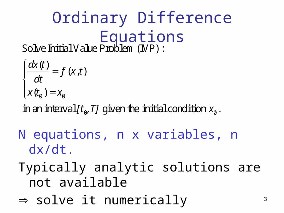
:(IVP) Problem Value Initial Solve
00
00
x,T][t
xtx
txfdt
tdx
N equations, n x variables, n dx/dt.
Typically analytic solutions are not available
solve it numerically
3
Numerical Integration
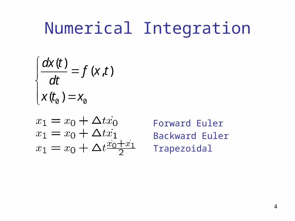
Forward Euler
Backward Euler
Trapezoidal
0 0
( )( , )
( )
dx tf x t
dtx t x
4
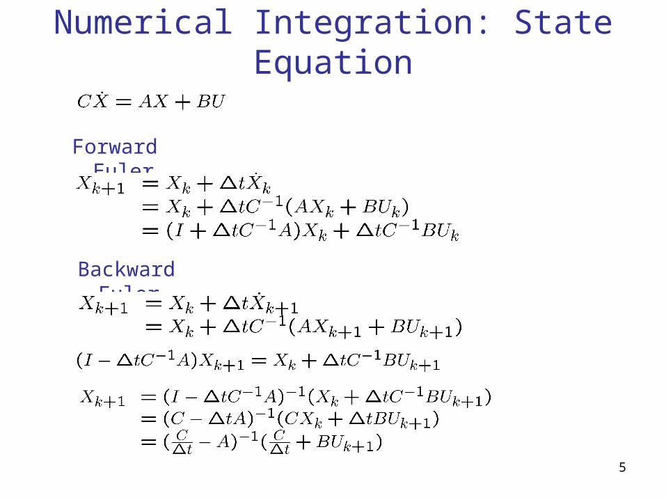
Numerical Integration: State Equation
Forward Euler
Backward Euler
5
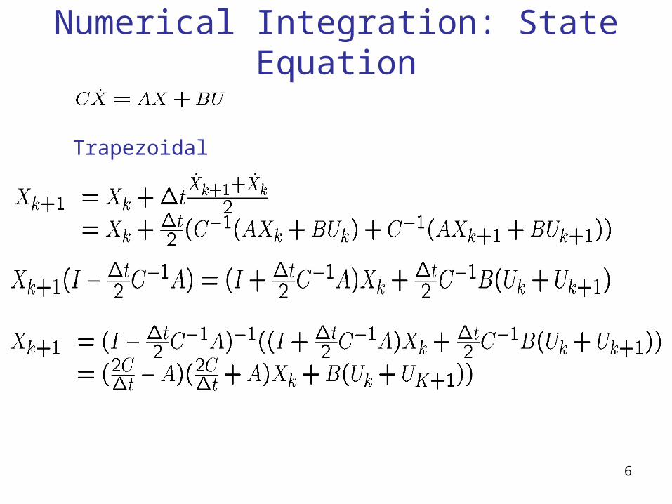
Numerical Integration: State Equation
Trapezoidal
6
7
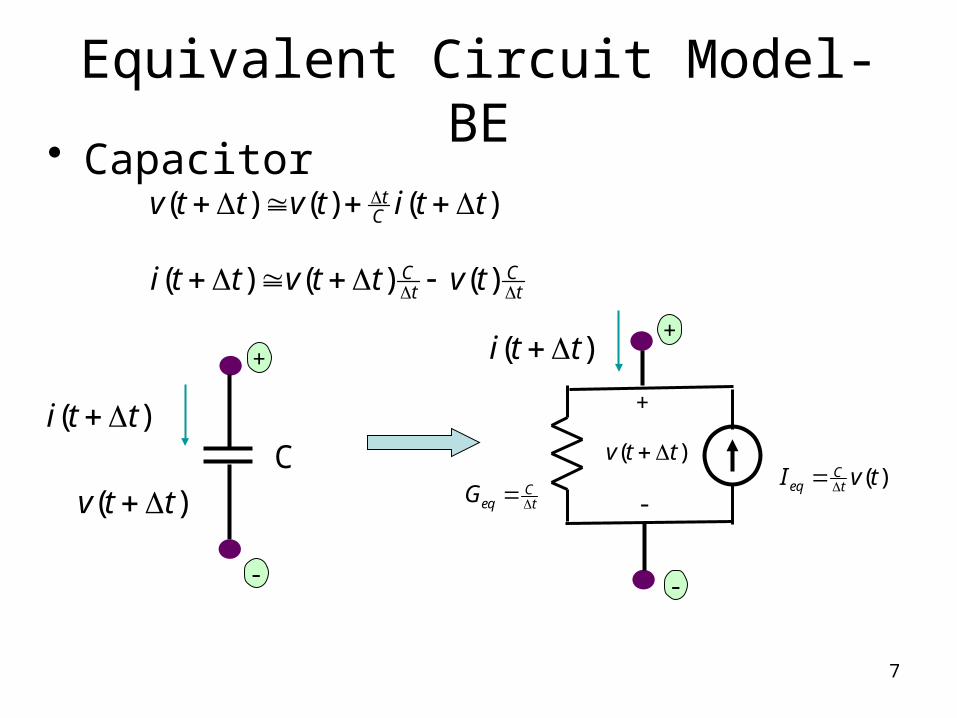
Equivalent Circuit Model-BE• Capacitor
( ) ( ) ( )tCv t t v t i t t
+
C
-
+
-
( )v t t
( )i t t
( )i t t
Ceq tG
( )v t t
+
-( )C
eq tI v t
( ) ( ) ( )C Ct ti t t v t t v t
8
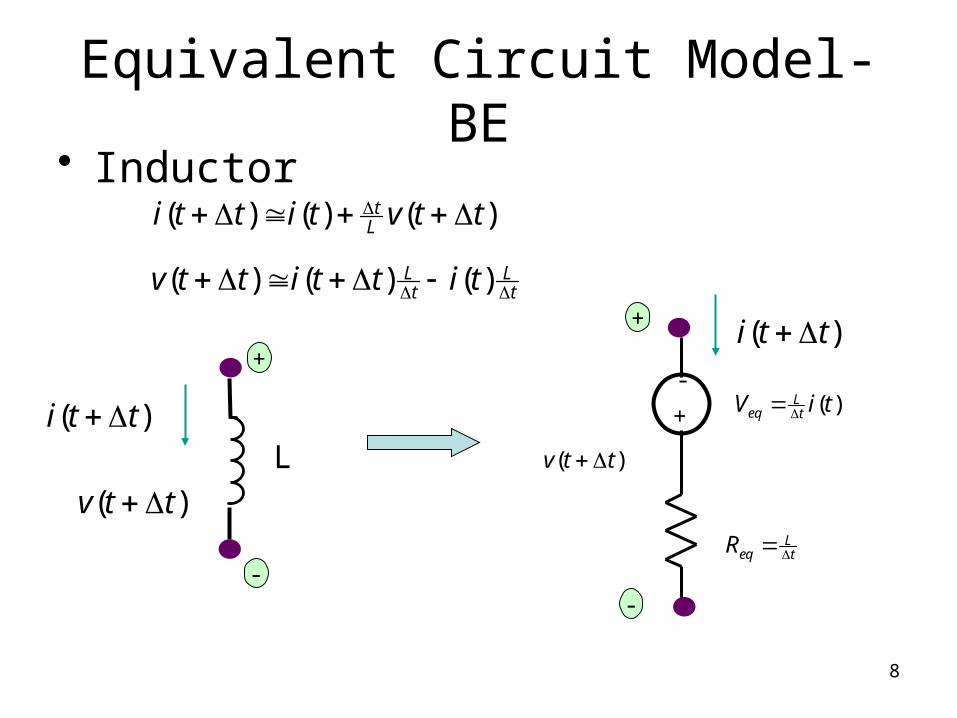
Equivalent Circuit Model-BE• Inductor
( ) ( ) ( )tLi t t i t v t t
+
L
-
+
-
( )v t t
( )i t t
( )i t t
Leq tR
( )v t t
+
-( )L
eq tV i t
( ) ( ) ( )L Lt tv t t i t t i t
9
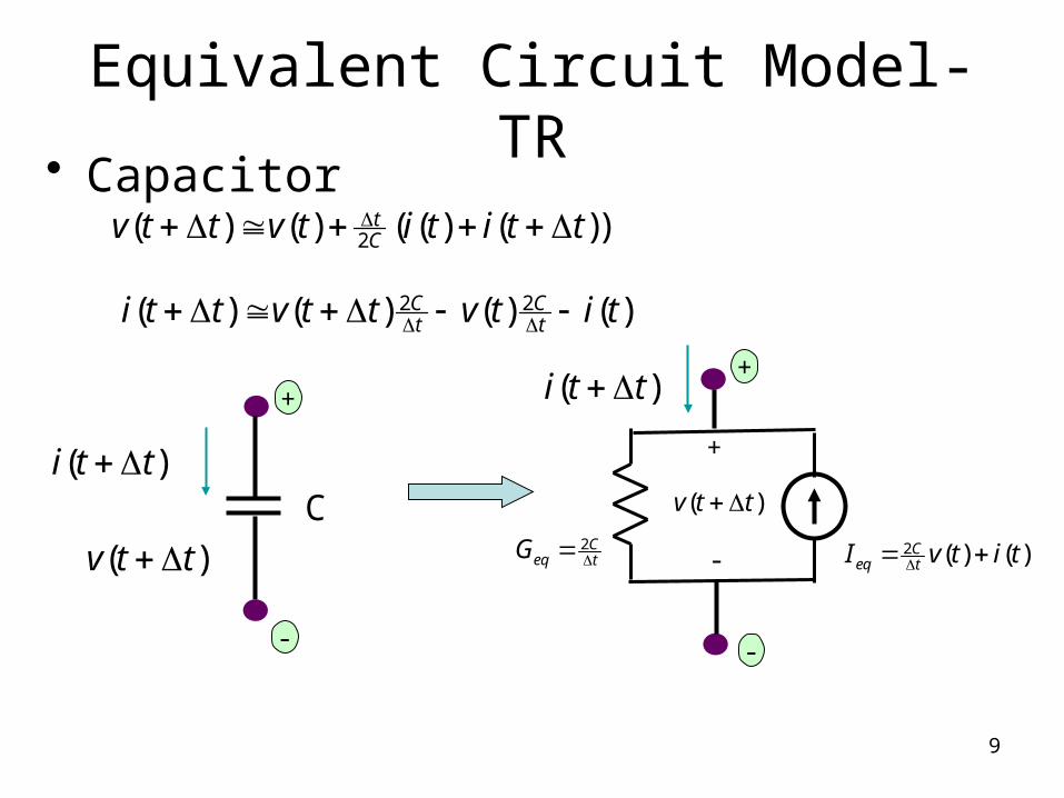
Equivalent Circuit Model-TR• Capacitor
2( ) ( ) ( ( ) ( ))tCv t t v t i t i t t
+
C
-
+
-
( )v t t
( )i t t
( )i t t
2Ceq tG
( )v t t
+
- 2 ( ) ( )Ceq tI v t i t
2 2( ) ( ) ( ) ( )C Ct ti t t v t t v t i t
10
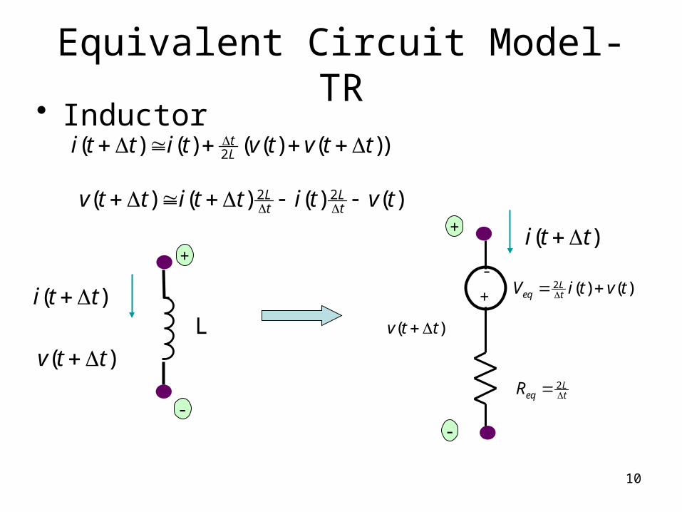
Equivalent Circuit Model-TR• Inductor
2( ) ( ) ( ( ) ( ))tLi t t i t v t v t t
+
L
-
+
-
( )v t t
( )i t t
( )i t t
2Leq tR
( )v t t
+
-2 ( ) ( )L
eq tV i t v t
2 2( ) ( ) ( ) ( )L Lt tv t t i t t i t v t
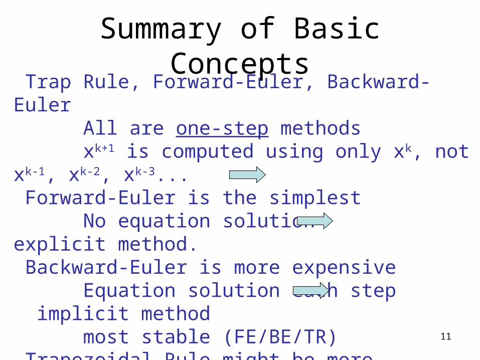
Trap Rule, Forward-Euler, Backward-Euler All are one-step methods xk+1 is computed using only xk, not xk-1, xk-2, xk-3... Forward-Euler is the simplest No equation solution explicit method. Backward-Euler is more expensive Equation solution each step implicit method most stable (FE/BE/TR) Trapezoidal Rule might be more accurate Equation solution each step implicit method More accurate but less stable, may cause oscillation
Summary of Basic Concepts
11
12
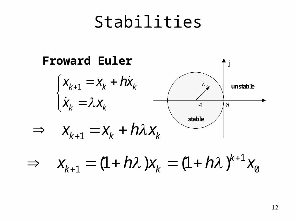
Stabilities
Froward Euler
0 -1
h
stable
unstable
j
1k k k
k k
x x hx
x x
1k k kx x h x
11 0(1 ) (1 )kk kx h x h x
Difference EqnStability region 1-1
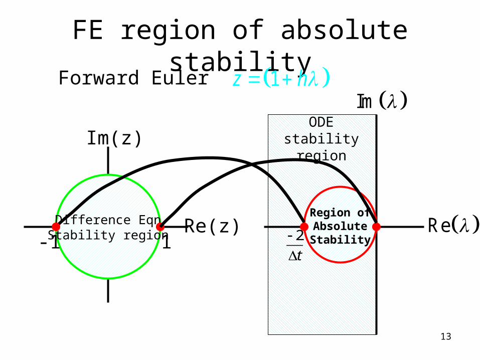
1z h
Im(z)
Re(z)
Im
Re
Forward Euler
ODE stability region
2
t
Region ofAbsolute Stability
FE region of absolute stability
13
14
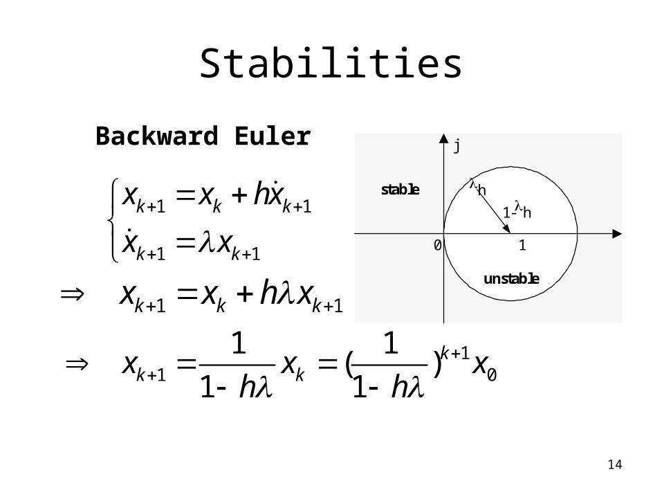
Stabilities
Backward Euler
1 1
1 1
k k k
k k
x x hx
x x
1 1k k kx x h x
11 0
1 1( )
1 1k
k kx x xh h
0 1
h
1-h
stable
unstable
j
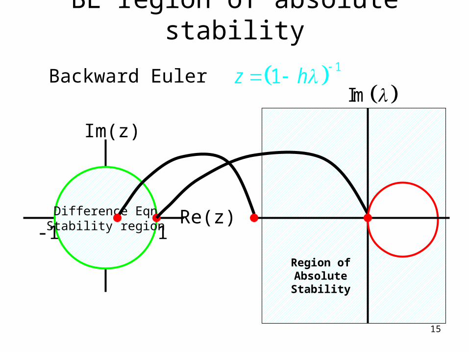
Difference EqnStability region 1-1
Im(z)
Re(z)
Im Backward Euler 1
1z h
Region ofAbsolute Stability
BE region of absolute stability
15
16
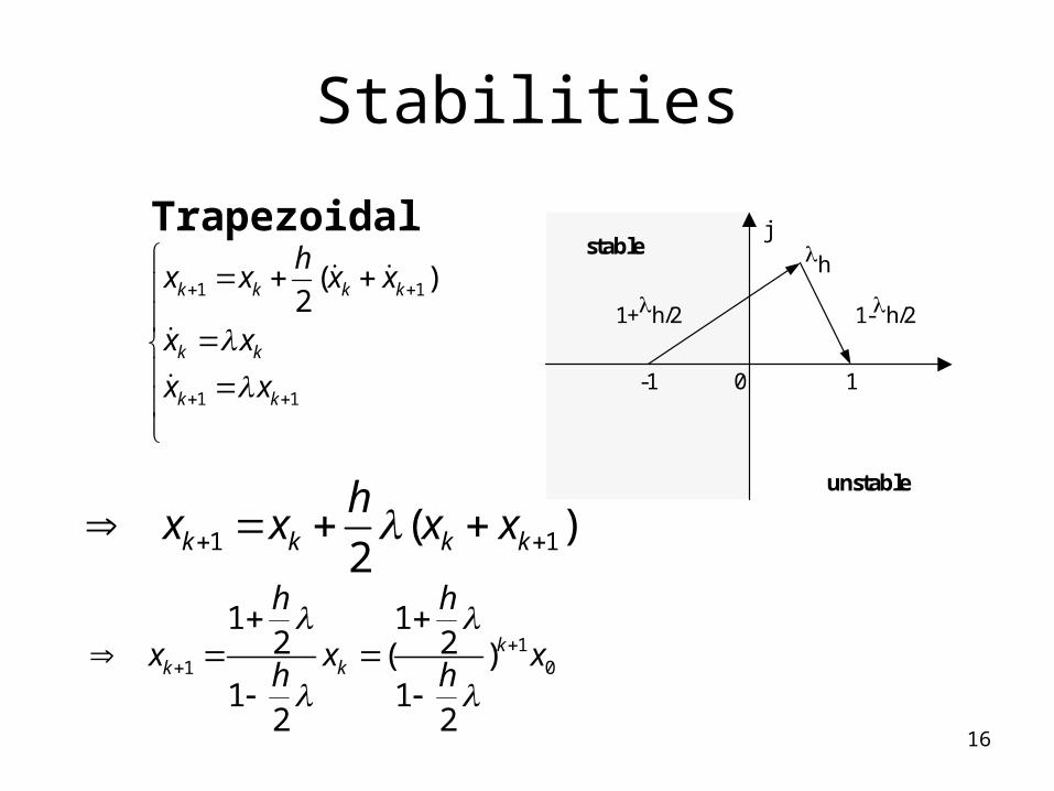
Stabilities
Trapezoidal
1 1
1 1
( )2k k k k
k k
k k
hx x x x
x x
x x
1 1( )2k k k k
hx x x x
11 0
1 12 2( )
1 12 2
kk k
h h
x x xh h
0 1
h
1+h/2
stable
unstable
-1
1-h/2
j
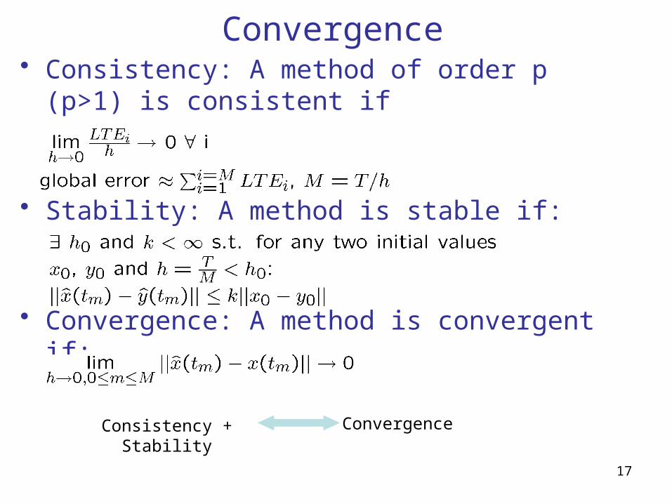
Convergence• Consistency: A method of order p (p>1) is
consistent if
• Stability: A method is stable if:
• Convergence: A method is convergent if:
Consistency + Stability Convergence
17
A-Stable
• Dahlquist Theorem:– An A-Stable LMS (Linear Multi-Step) method
cannot exceed 2nd order accuracy• The most accurate A-Stable method
(smallest truncation error) is trapezoidal method.
18
Convergence Analysis: Truncation Error
• Local Truncation Error (LTE):– At time point tk+1 assume xk is exact, the difference between
the approximated solution xk+1 and exact solution x*k+1 is called
local truncation error.– Indicates consistency– Used to estimate next time step size in SPICE
• Global Truncation Error (GTE):– At time point tk+1, assume only the initial condition x0 at time t0
is correct, the difference between the approximated solution xk+1 and the exact solution x*
k+1 is called global truncation error.
– Indicates stability
19
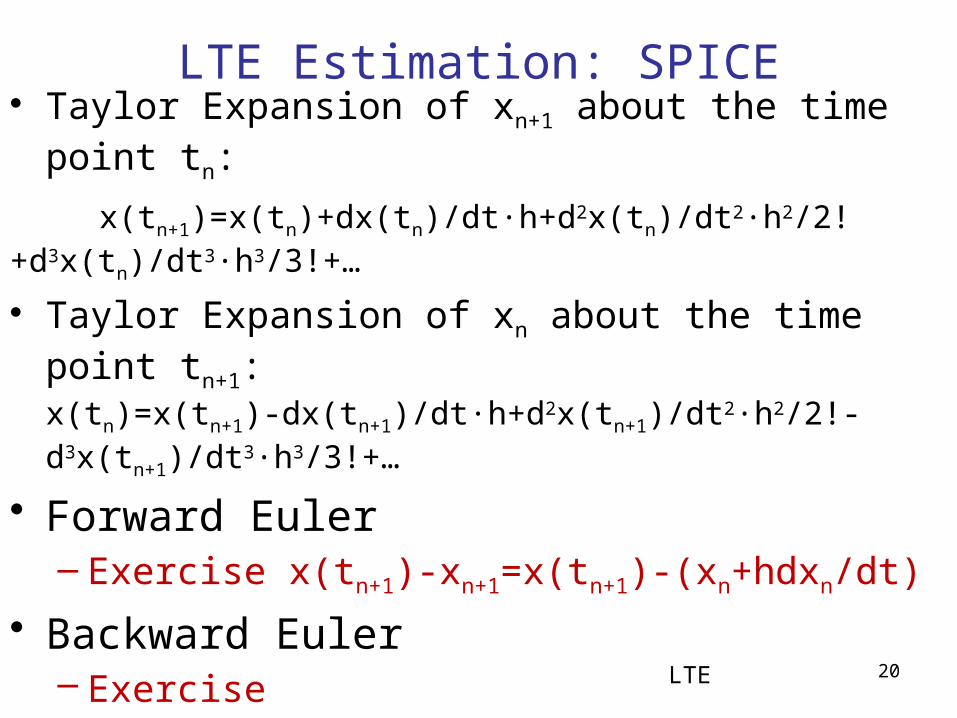
LTE Estimation: SPICE• Taylor Expansion of xn+1 about the time point tn:
x(tn+1)=x(tn)+dx(tn)/dt∙h+d2x(tn)/dt2∙h2/2!+d3x(tn)/dt3∙h3/3!+…
• Taylor Expansion of xn about the time point tn+1: x(tn)=x(tn+1)-dx(tn+1)/dt∙h+d2x(tn+1)/dt2∙h2/2!-d3x(tn+1)/dt3∙h3/3!+…
• Forward Euler– Exercise x(tn+1)-xn+1=x(tn+1)-(xn+hdxn/dt)
• Backward Euler– Exercise x(tn+1)-xn+1=x(tn+1)-(xn+hdxn+1/dt)
• Trapezoidal– Exercise x(tn+1)-xn+1=x(tn+1)-[xn+(dxn/dt+dxn+1/dt)h/2]
LTE 20
Formula for pth order method
LTE 21
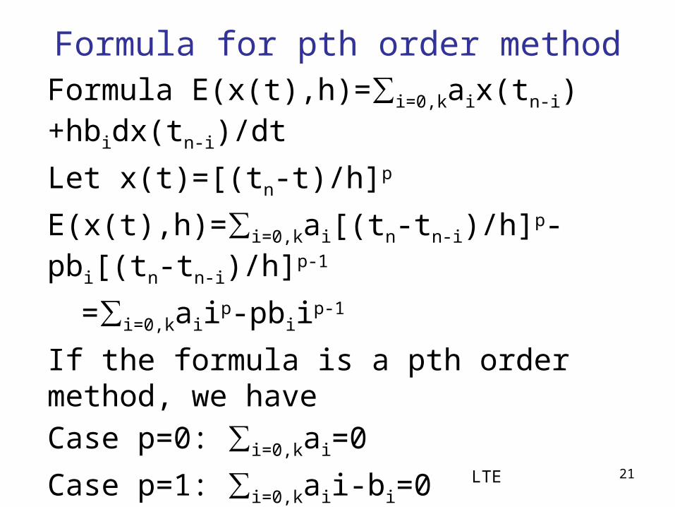
Formula E(x(t),h)=∑i=0,kaix(tn-i)+hbidx(tn-i)/dt
Let x(t)=[(tn-t)/h]p
E(x(t),h)=∑i=0,kai[(tn-tn-i)/h]p-pbi[(tn-tn-i)/h]p-1
=∑i=0,kaiip-pbiip-1
If the formula is a pth order method, we have
Case p=0: ∑i=0,kai=0
Case p=1: ∑i=0,kaii-bi=0
……
Case p: ∑i=0,k(aii-pbi)ip-1=0
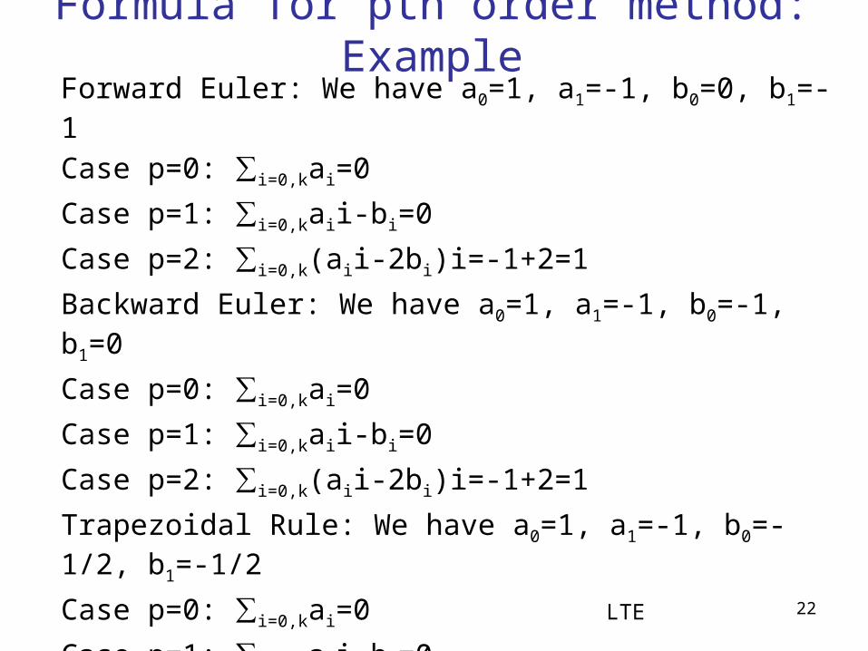
Formula for pth order method: Example
LTE 22
Forward Euler: We have a0=1, a1=-1, b0=0, b1=-1
Case p=0: ∑i=0,kai=0
Case p=1: ∑i=0,kaii-bi=0
Case p=2: ∑i=0,k(aii-2bi)i=-1+2=1
Backward Euler: We have a0=1, a1=-1, b0=-1, b1=0
Case p=0: ∑i=0,kai=0
Case p=1: ∑i=0,kaii-bi=0
Case p=2: ∑i=0,k(aii-2bi)i=-1+2=1
Trapezoidal Rule: We have a0=1, a1=-1, b0=-1/2, b1=-1/2
Case p=0: ∑i=0,kai=0
Case p=1: ∑i=0,kaii-bi=0
Case p=2: ∑i=0,k(aii-2bi)i=0
Case p=3: ∑i=0,k(aii-3bi)i2=-1+3/2=1/2
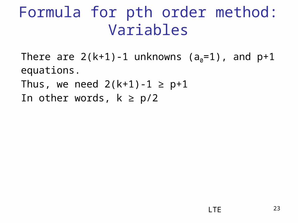
Formula for pth order method: Variables
LTE 23
There are 2(k+1)-1 unknowns (a0=1), and p+1 equations.
Thus, we need 2(k+1)-1 ≥ p+1
In other words, k ≥ p/2
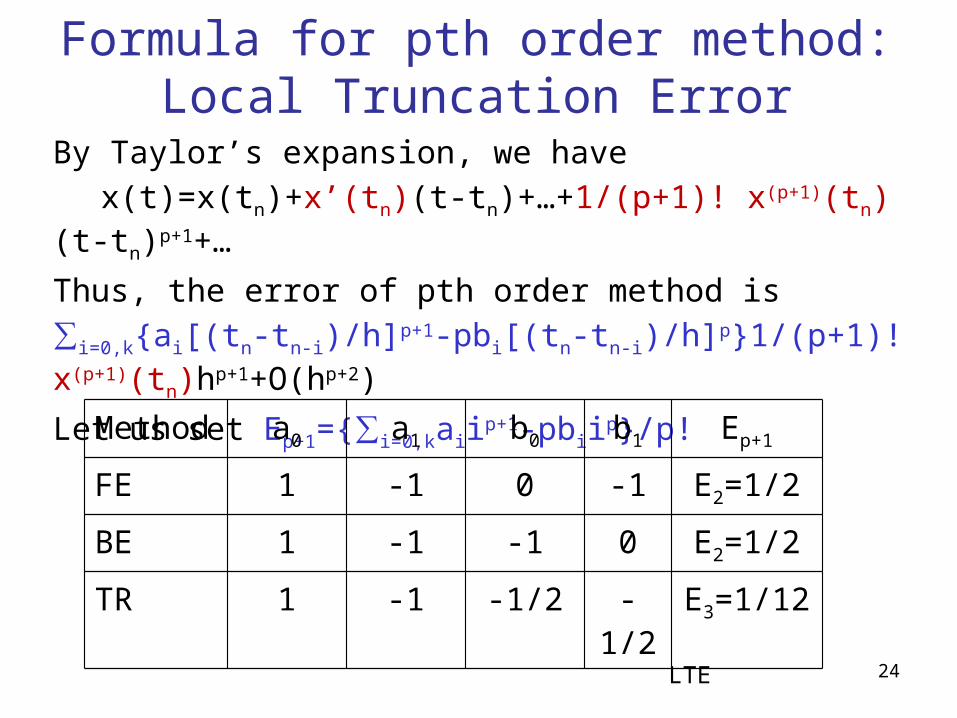
Formula for pth order method: Local Truncation Error
LTE 24
By Taylor’s expansion, we have
x(t)=x(tn)+x’(tn)(t-tn)+…+1/(p+1)! x(p+1)(tn)(t-tn)p+1+…
Thus, the error of pth order method is
∑i=0,k{ai[(tn-tn-i)/h]p+1-pbi[(tn-tn-i)/h]p}1/(p+1)! x(p+1)(tn)hp+1+O(hp+2)
Let us set Ep+1={∑i=0,kaiip+1-pbiip}/p!
Method a0 a1 b0 b1 Ep+1
FE 1 -1 0 -1 E2=1/2
BE 1 -1 -1 0 E2=1/2
TR 1 -1 -1/2 -1/2 E3=1/12
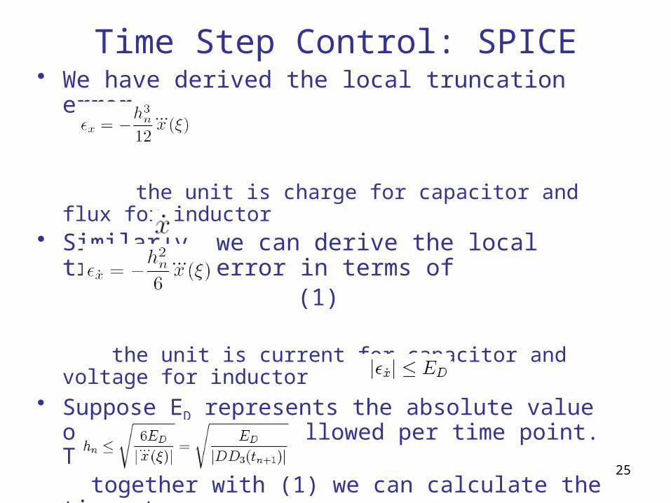
Time Step Control: SPICE• We have derived the local truncation error
the unit is charge for capacitor and flux for inductor• Similarly, we can derive the local truncation error in
terms of (1)
the unit is current for capacitor and voltage for inductor• Suppose ED represents the absolute value of error that is
allowed per time point. That is together with (1) we can calculate the time step as
25
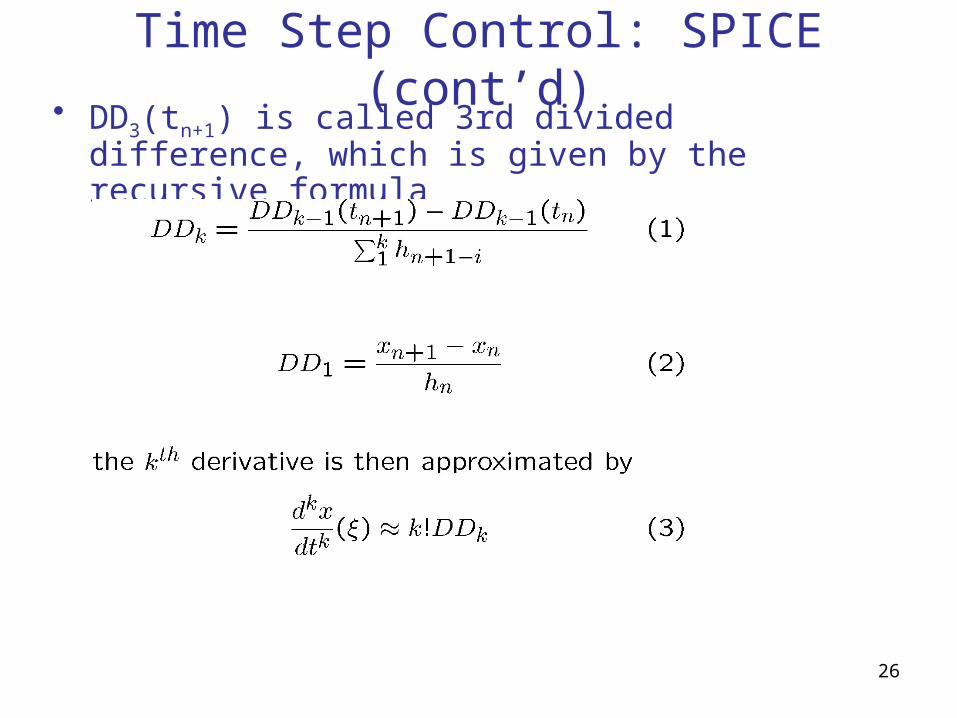
Time Step Control: SPICE (cont’d)• DD3(tn+1) is called 3rd divided difference, which is given
by the recursive formula
26
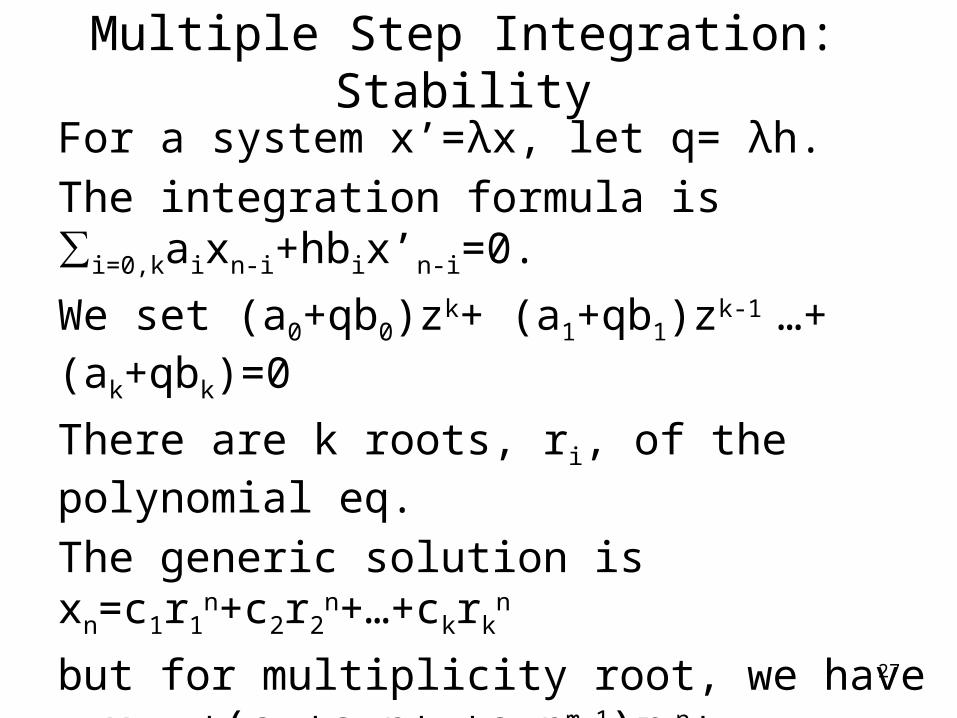
Multiple Step Integration: Stability
For a system x’=λx, let q= λh.
The integration formula is ∑i=0,kaixn-i+hbix’n-i=0.
We set (a0+qb0)zk+ (a1+qb1)zk-1 …+(ak+qbk)=0
There are k roots, ri, of the polynomial eq.
The generic solution is xn=c1r1n+c2r2
n+…+ckrkn
but for multiplicity root, we have xn=…+(ci0+ci1n+…+cimnm-1)ri
n+…
If |ri|< 1 for all i, the system is stable
Else for |ri|= 1 but not multiplicity root, the system remains stable
27
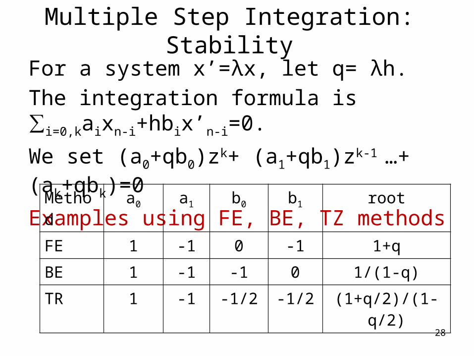
Multiple Step Integration: Stability
For a system x’=λx, let q= λh.
The integration formula is ∑i=0,kaixn-i+hbix’n-i=0.
We set (a0+qb0)zk+ (a1+qb1)zk-1 …+(ak+qbk)=0
Examples using FE, BE, TZ methods
28
Method a0 a1 b0 b1 root
FE 1 -1 0 -1 1+q
BE 1 -1 -1 0 1/(1-q)
TR 1 -1 -1/2 -1/2 (1+q/2)/(1-q/2)
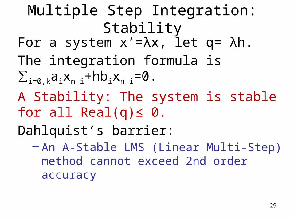
Multiple Step Integration: Stability
For a system x’=λx, let q= λh.
The integration formula is ∑i=0,kaixn-i+hbixn-i=0.
A Stability: The system is stable for all Real(q)≤ 0.
Dahlquist’s barrier:– An A-Stable LMS (Linear Multi-Step) method
cannot exceed 2nd order accuracy
29