Embed Size (px)
Citation preview
cs/ee 143 Communication Networks
Steven Low CMS, EE, Caltech
Fall 2012
Introduction to Communication Networks
Steven Low Caltech, Zhejiang University
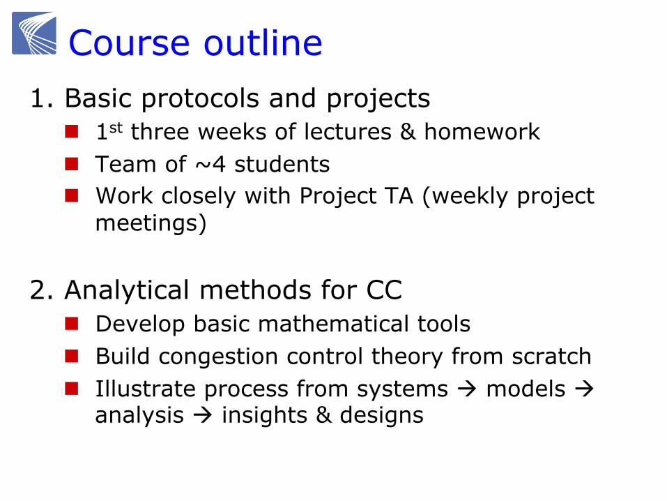
Course outline 1. Basic protocols and projects
n 1st three weeks of lectures & homework n Team of ~4 students n Work closely with Project TA (weekly project
meetings)
2. Analytical methods for CC n Develop basic mathematical tools n Build congestion control theory from scratch n Illustrate process from systems à models à
analysis à insights & designs
Warning
These notes are not self-contained, probably not understandable,
unless you also were in the lecture They are supplement to not replacement for class attendance
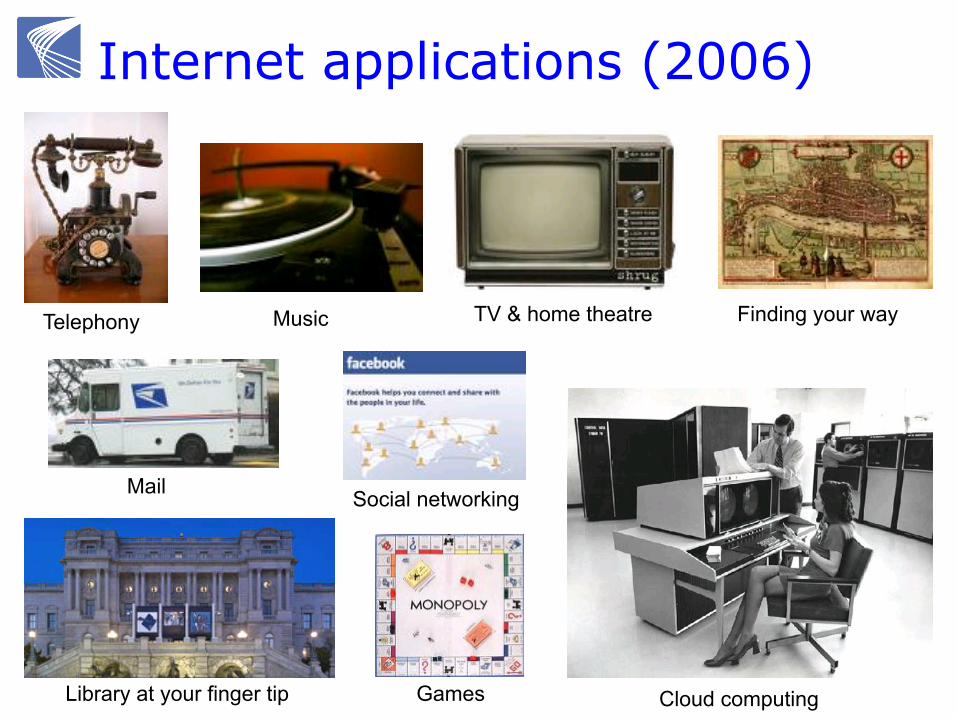
Internet applications (2006)
Telephony Music TV & home theatre
Cloud computing
Finding your way
Games Library at your finger tip
Social networking
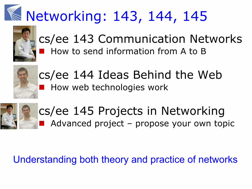
Networking: 143, 144, 145 o cs/ee 143 Communication Networks
n How to send information from A to B
o cs/ee 144 Ideas Behind the Web n How web technologies work
o cs/ee 145 Projects in Networking n Advanced project – propose your own topic
Understanding both theory and practice of networks
Networking: 143, 144, 145 143: transport layer and down 144: transport layer and up 145: project course 143/144/145 forms a project sequence for CS major
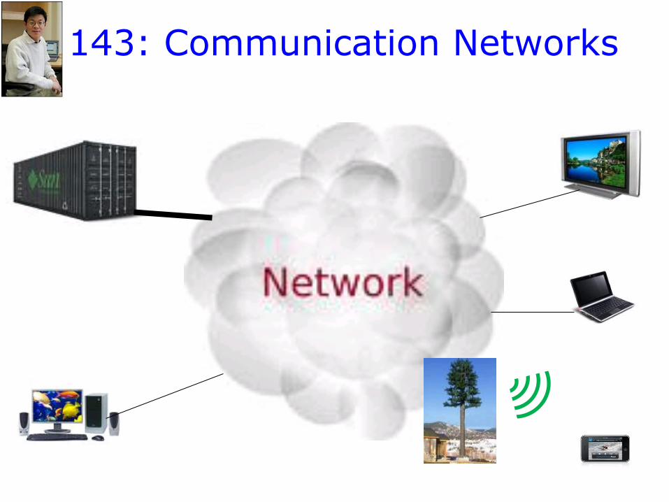
143: Communication Networks

144: Ideas behind the web a.k.a. What makes google tick?
Unique course that you can’t find at any other school
The course will be a series of important topics from the web. For each, we will learn - The theory behind the topic - Hands-on design, system building
CS 141a - Distributed Computation Laboratory Course Introduction http://www.cs.caltech.edu/~cs141/ 2 October 2007 10
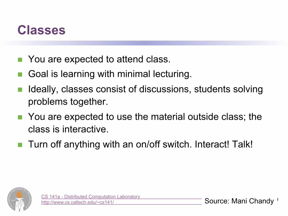
Classes
n You are expected to attend class. n Goal is learning with minimal lecturing. n Ideally, classes consist of discussions, students solving
problems together. n You are expected to use the material outside class; the
class is interactive. n Turn off anything with an on/off switch. Interact! Talk!
Source: Mani Chandy

Alumni Recommendation
n The Caltech experience should give engineers skills in: n Communication
n Writing scientific papers, proposals, plans n Speaking to science, government, business
audiences n Working in teams
n Project planning and management n Division of labor; leadership n Larger, global view of the world
Source: Mani Chandy
RSRG courses and research
RSRG courses 1. Learn by doing
1. Emphasis on creativity, problem-solving, research
2. Integrating courses, SURF, internships, theses, research opportunities in multiyear programs
3. Close interaction with faculty in and out of class 4. Interactive classes: “The lecture is dead.” [ideal]
Source: Mani Chandy

Course website
http://courses.cms.caltech.edu/cs143/
cs/ee 143 Communication Networks Chapter 1 The Internet
Text: Walrand & Parakh, 2010
Steven Low CMS, EE, Caltech
2 1. THE INTERNET
128.132.154.46
169.229.60.32 = A�
coeus.eecs.berkeley.edu 18.7.25.81�
sloan.mit.edu
128
169 18 18.64
18169
18.128.33.11
18.12864
169
110.27.36.91= B
64
64
[A|B| ... |CRC]
R1 R2
R3
L1
L2
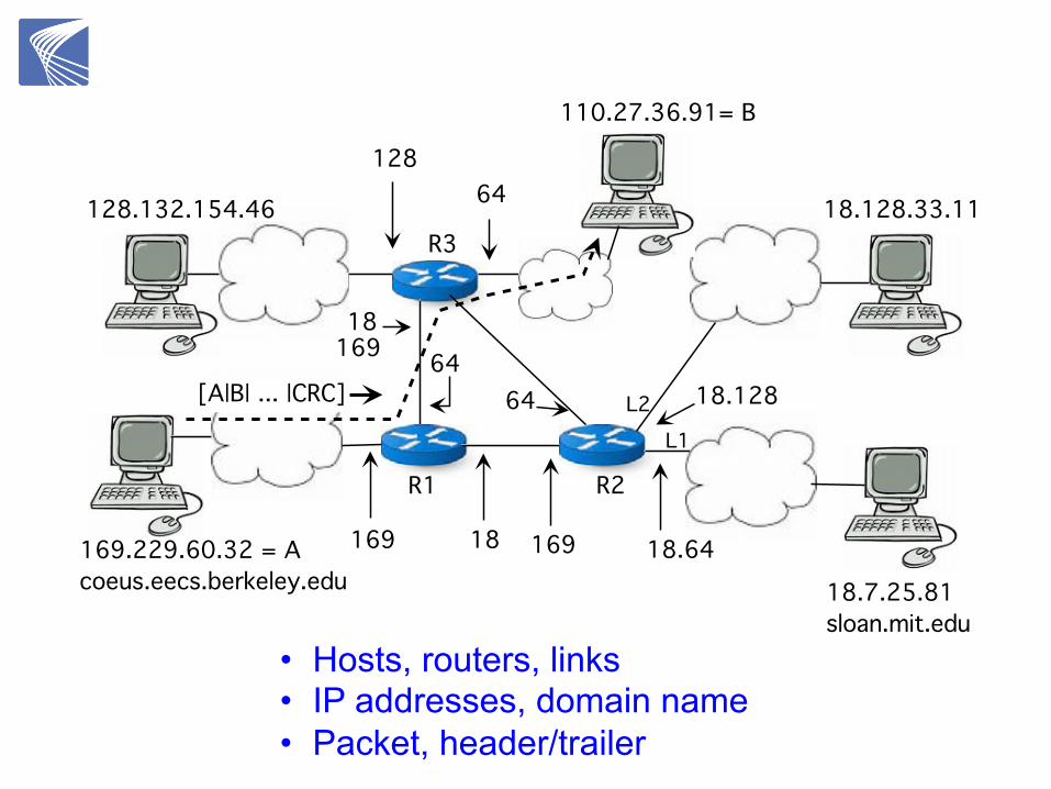
Figure 1.1: Hosts, routers, and links. Each host has a distinct location-based 32-bit IP address. The
packet header contains the source and destination addresses and an error checksum. The routers
maintain routing tables that specify the output for the longest prefix match of the destination
address.
1.1.3 ADDRESSINGEvery computer or other host attached to the Internet has a unique address specified by a 32-bitstring called its IP address, for Internet Protocol Address. The addresses are conventionally written inthe form a.b.c.d where a, b, c, d are the decimal value of the four bytes. For instance, 169.229.60.32corresponds to the four bytes 10101001.11100101.00111100.00100000.
1.1.4 ROUTINGEach router determines the next hop for the packet from the destination address. While advancingtowards the destination, within a network under the control of a common administrator, the packetsessentially follow the shortest path. 1 The routers regularly compute these shortest paths and recordthem as routing tables. 2 A routing table specifies the next hop for each destination address, assketched in Figure 1.2.
1The packets typically go through a set of networks that belong to different organizations. The routers select this set of networksaccording to rules that we discuss in the Routing chapter.
2More precisely, the router consults a forwarding table that indicates the output port of the packet. However, this distinction is notessential.
• Hosts, routers, links • IP addresses, domain name • Packet, header/trailer
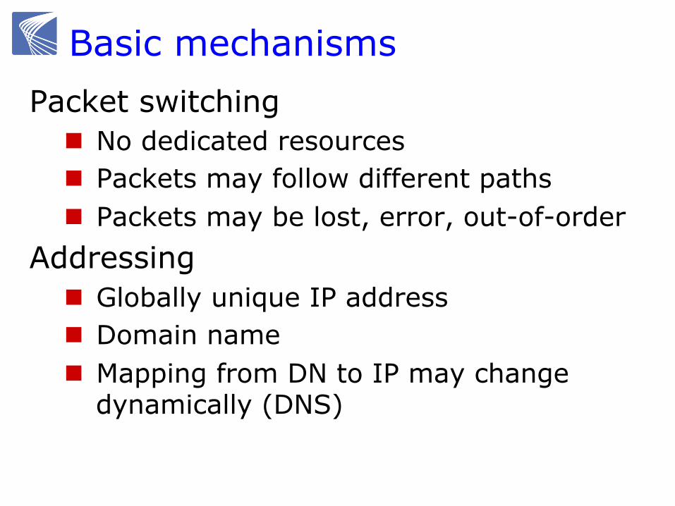
Basic mechanisms Packet switching
n No dedicated resources n Packets may follow different paths n Packets may be lost, error, out-of-order
Addressing n Globally unique IP address n Domain name n Mapping from DN to IP may change
dynamically (DNS)
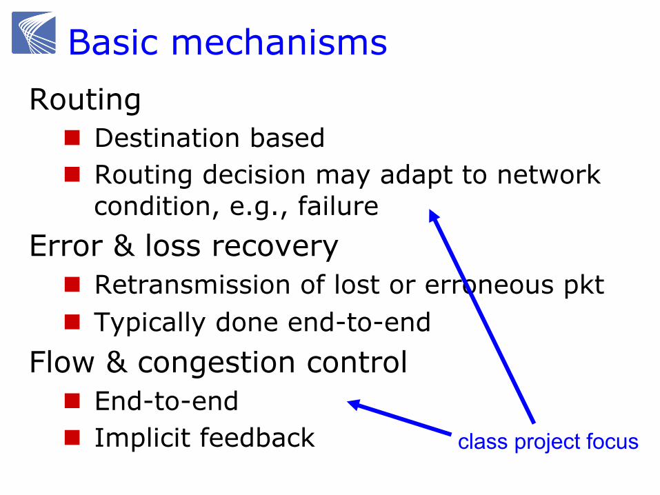
Basic mechanisms Routing
n Destination based n Routing decision may adapt to network
condition, e.g., failure Error & loss recovery
n Retransmission of lost or erroneous pkt n Typically done end-to-end
Flow & congestion control n End-to-end n Implicit feedback class project focus
Router 1.1. BASIC OPERATIONS 3
S | D | …
D port 1F port 2K port 16
Routing Table
Input Ports Output Ports
1
2
32
1
2
32
SourceDestination
Destination
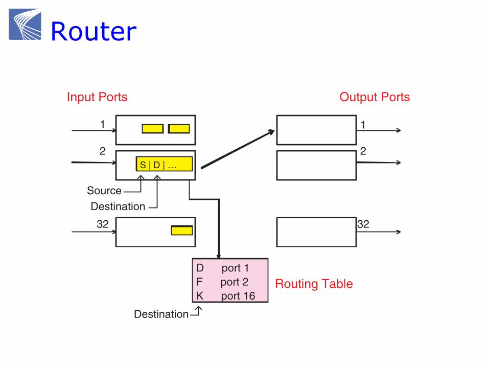
Figure 1.2: The figure sketches a router with 32 input ports (link attachments) and 32 output ports.
Packets contain their source and destination addresses. A routing table specifies, for each destination,
the corresponding output port for the packet.
To simplify the routing tables, the network administrators assign IP addresses to hosts basedon their location. For instance, router R1 in Figure 1.1 sends all the packets with a destinationaddress whose first byte has decimal value 18 to router R2 and all the packets with a destinationaddress whose first byte has decimal value 64 to router R3. Instead of having one entry for everypossible destination address, a router has one entry for a set of addresses with a common initial bitstring, or prefix. If one could assign addresses so that all the destinations that share the same initialfive bits were reachable from the same port of a 32-port router, then the routing table of the routerwould need only 32 entries of 5 bits: each entry would specify the initial five bits that correspondto each port. In practice, the assignment of addresses is not perfectly regular, but it neverthelessreduces considerably the size of routing tables. This arrangement is quite similar to the organizationof telephone numbers into [country code, area code, zone, number]. For instance, the number 1 510642 1529 corresponds to a telephone set in the US (1), in Berkeley (510), the zone of the Berkeleycampus (642).
The general approach to exploit location-based addressing is to find the longest commoninitial string of bits (called prefix) in the addresses that are reached through the same next hop.This scheme, called Classless Interdomain Routing (or CIDR), enables to arrange the addresses intosubgroups identified by prefixes in a flexible way.The main difference with the telephone numberingscheme is that, in CIDR, the length of the prefix is not predetermined, thus providing more flexibility.
As an illustration of longest prefix match routing, consider how router R2 in Figure 1.1 selectswhere to send packets. A destination address that starts with the bits 000010101 matches the first 9bits of the prefix 18.128 = 00010010’10000000 of output link L2 but only the first 8 bits of the prefix
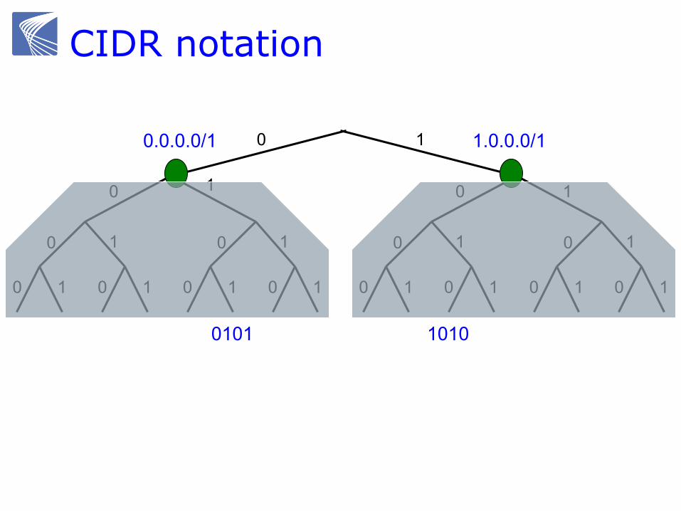
CIDR notation
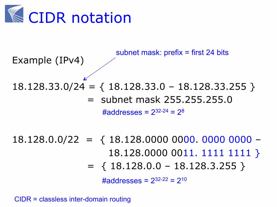
Example (IPv4) 18.128.33.0/24 = { 18.128.33.0 – 18.128.33.255 }
= subnet mask 255.255.255.0 18.128.0.0/22 = { 18.128.0000 0000. 0000 0000 –
18.128.0000 0011. 1111 1111 } = { 18.128.0.0 – 18.128.3.255 }
subnet mask: prefix = first 24 bits
#addresses = 232-24 = 28
#addresses = 232-22 = 210
CIDR = classless inter-domain routing
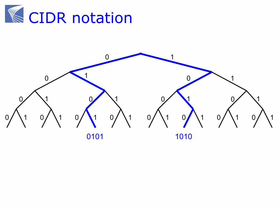
CIDR notation
0101
1 0
0 1
0 1
0 1 0 1
0 1
0 1
0
0 1
0 1
0 1 0 1
0 1
0 1
0
1
1
1010
CIDR notation
0101
1 0
0 1
0 1
0 1 0 1
0 1
0 1
0
0 1
0 1
0 1 0 1
0 1
0 1
0
1
1
1010
0.0.0.0/1 1.0.0.0/1
CIDR notation
0101
1 0
0 1
0 1
0 1 0 1
0 1
0 1
0
0 1
0 1
0 1 0 1
0 1
0 1
0
1
1
1010
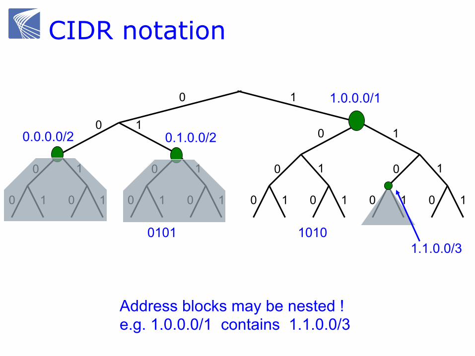
0.0.0.0/2
1.0.0.0/1
0.1.0.0/2
1.1.0.0/3
Address blocks may be nested ! e.g. 1.0.0.0/1 contains 1.1.0.0/3
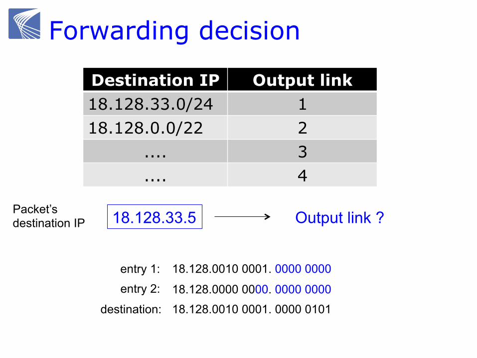
Forwarding decision
Destination IP Output link 18.128.33.0/24 1 18.128.0.0/22 2
.... 3
.... 4
18.128.33.5 Packet’s destination IP Output link ?
18.128.0010 0001. 0000 0000
18.128.0000 0000. 0000 0000
18.128.0010 0001. 0000 0101
entry 1:
entry 2:
destination:
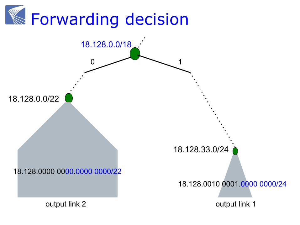
Forwarding decision
0 1
18.128.0.0/18
18.128.0.0/22
18.128.33.0/24
18.128.0010 0001.0000 0000/24
18.128.0000 0000.0000 0000/22
output link 2 output link 1
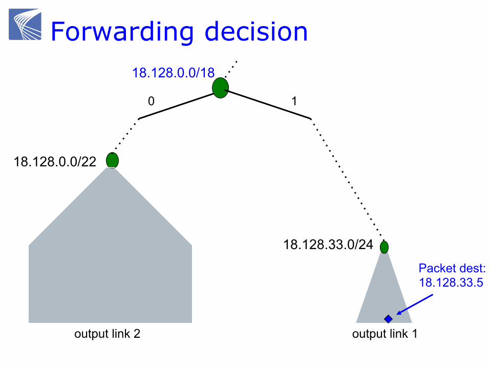
Forwarding decision
0 1
18.128.0.0/18
18.128.0.0/22
18.128.33.0/24
Packet dest: 18.128.33.5
output link 2 output link 1

Longest prefix matching
Destination IP Output link 18.128.33.0/24 1 18.128.0.0/22 2
.... 3
.... 4
18.128.33.5 Packet’s destination IP Output link 1
It matches only the first address block
18.128.0010 0001. 0000 0000
18.128.0000 0000. 0000 0000
18.128.0010 0001. 0000 0101
entry 1:
entry 2:
destination:
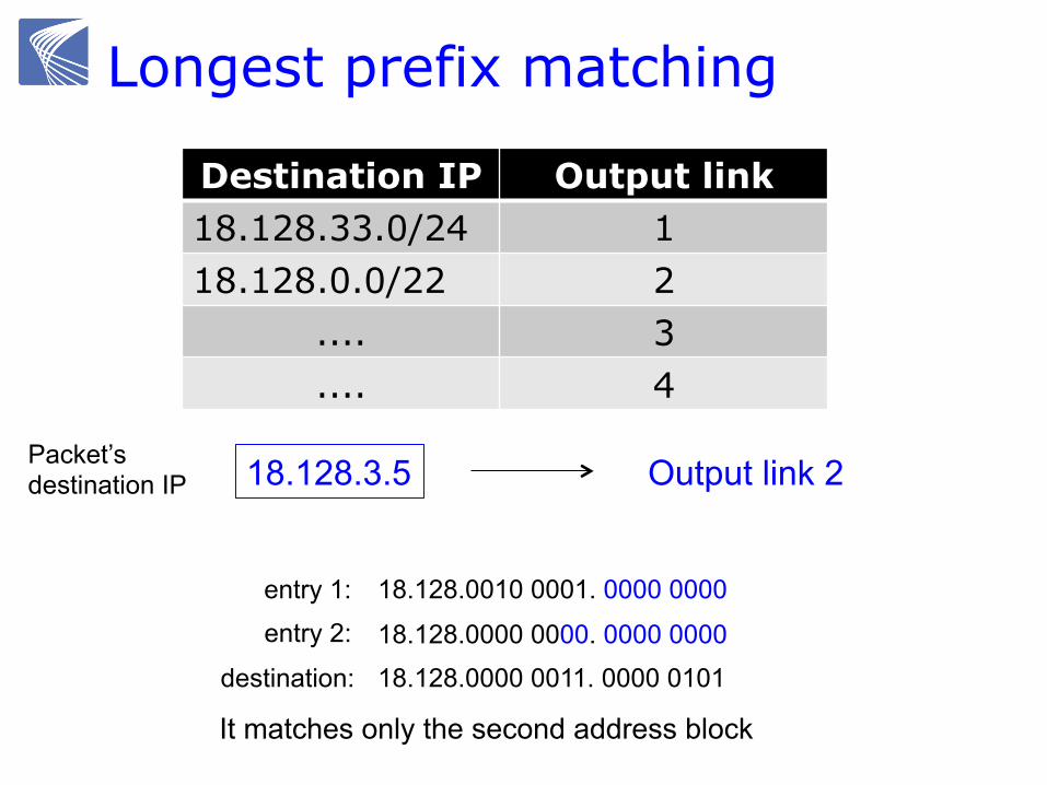
Longest prefix matching
Destination IP Output link 18.128.33.0/24 1 18.128.0.0/22 2
.... 3
.... 4
18.128.3.5 Packet’s destination IP Output link 2
It matches only the second address block
18.128.0010 0001. 0000 0000
18.128.0000 0000. 0000 0000
18.128.0000 0011. 0000 0101
entry 1:
entry 2:
destination:
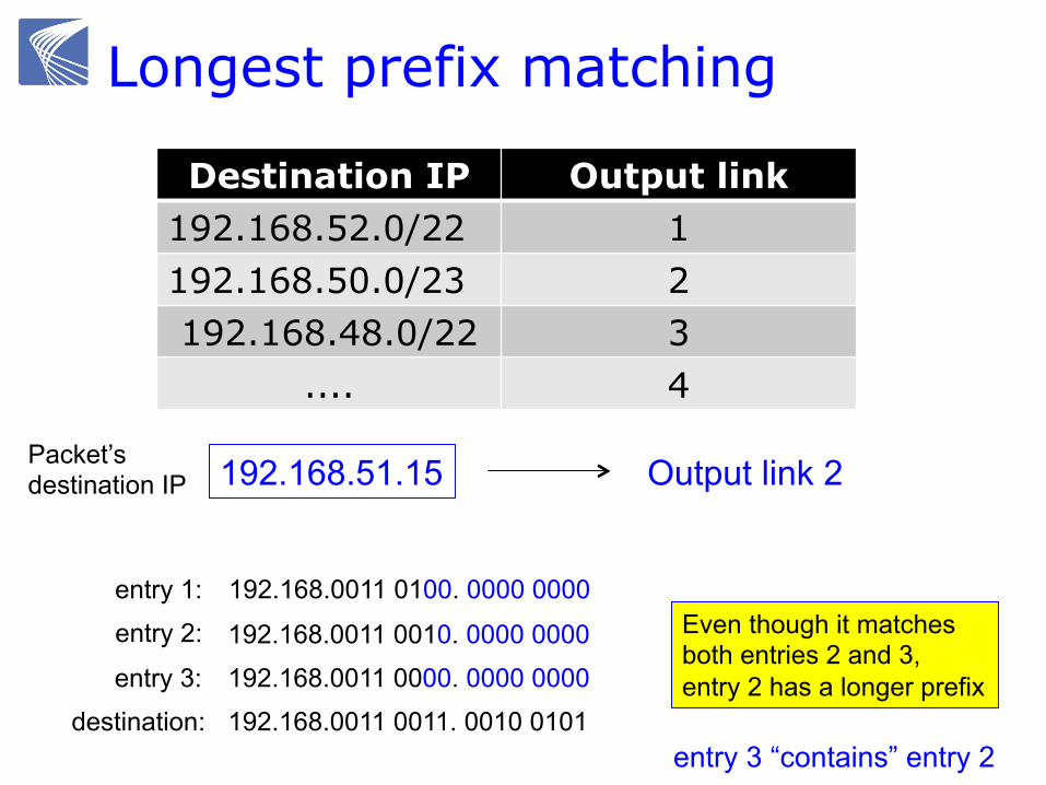
Longest prefix matching
Destination IP Output link 192.168.52.0/22 1 192.168.50.0/23 2 192.168.48.0/22 3
.... 4
192.168.51.15 Packet’s destination IP Output link 2
192.168.0011 0100. 0000 0000 entry 1:
entry 2:
entry 3:
192.168.0011 0010. 0000 0000
192.168.0011 0000. 0000 0000
destination: 192.168.0011 0011. 0010 0101
Even though it matches both entries 2 and 3, entry 2 has a longer prefix
entry 3 “contains” entry 2
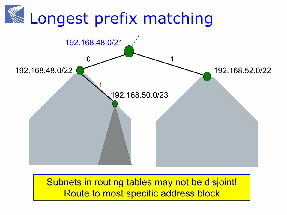
Longest prefix matching
0 1
192.168.48.0/21
192.168.48.0/22
1 192.168.50.0/23
192.168.52.0/22
Subnets in routing tables may not be disjoint! Route to most specific address block
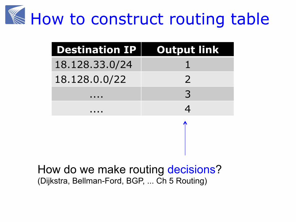
How to construct routing table
Destination IP Output link 18.128.33.0/24 1 18.128.0.0/22 2
.... 3
.... 4
How do we make routing decisions? (Dijkstra, Bellman-Ford, BGP, ... Ch 5 Routing)
cs/ee 143 Communication Networks Chapter 2 Principles
Text: Walrand & Parakh, 2010
Steven Low CMS, EE, Caltech
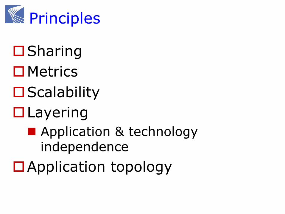
Principles
o Sharing o Metrics o Scalability o Layering
n Application & technology independence
o Application topology
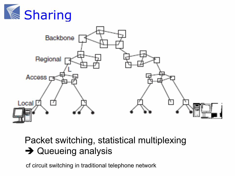
Sharing
Packet switching, statistical multiplexing è Queueing analysis cf circuit switching in traditional telephone network
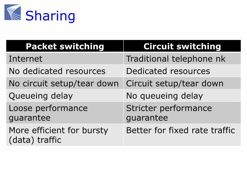
Sharing
Packet switching Circuit switching Internet Traditional telephone nk No dedicated resources Dedicated resources No circuit setup/tear down Circuit setup/tear down Queueing delay No queueing delay Loose performance guarantee
Stricter performance guarantee
More efficient for bursty (data) traffic
Better for fixed rate traffic
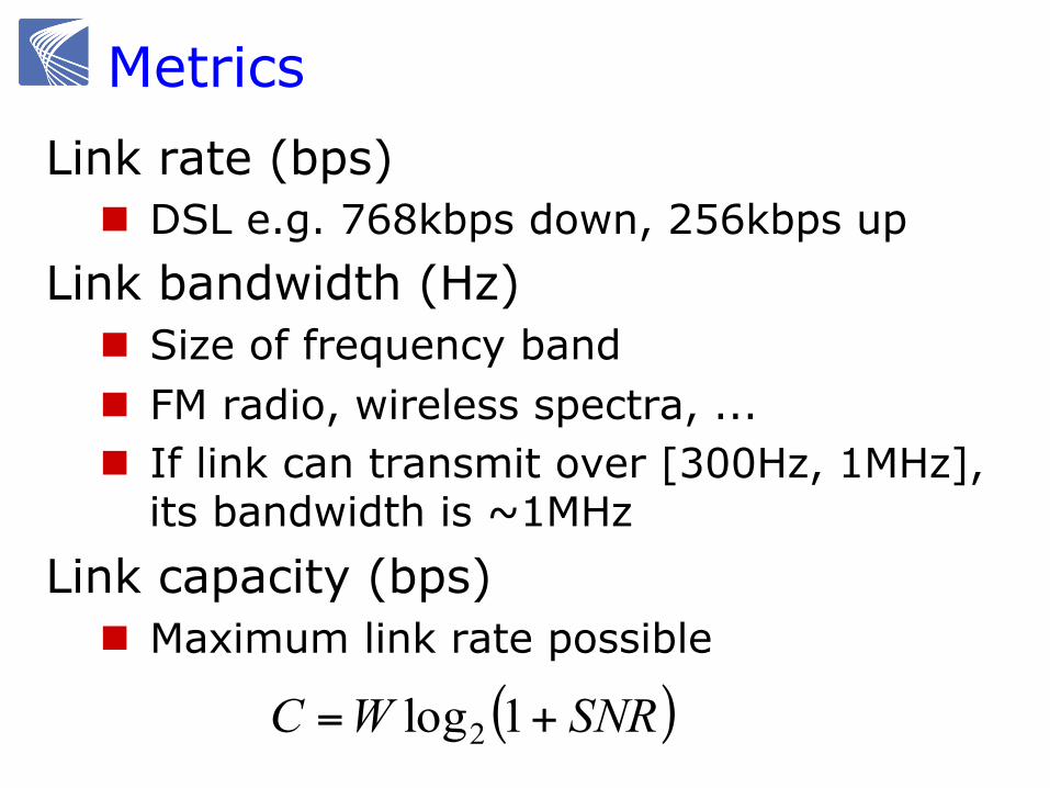
Metrics Link rate (bps)
n DSL e.g. 768kbps down, 256kbps up Link bandwidth (Hz)
n Size of frequency band n FM radio, wireless spectra, ... n If link can transmit over [300Hz, 1MHz],
its bandwidth is ~1MHz Link capacity (bps)
n Maximum link rate possible
( )SNRWC += 1log2
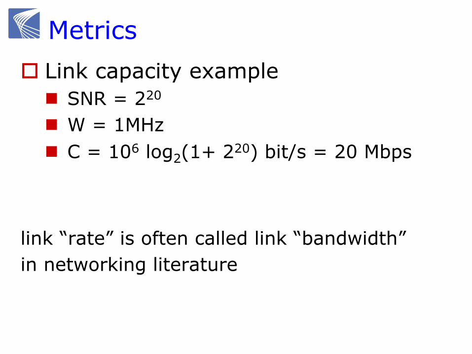
Metrics o Link capacity example
n SNR = 220
n W = 1MHz n C = 106 log2(1+ 220) bit/s = 20 Mbps
link “rate” is often called link “bandwidth” in networking literature
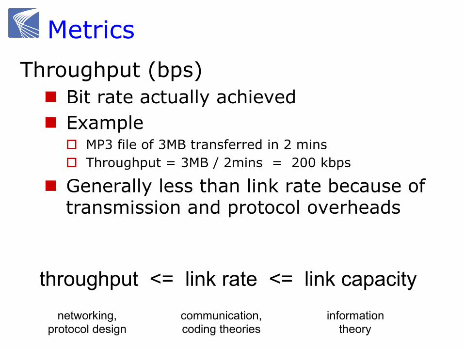
Metrics Throughput (bps)
n Bit rate actually achieved n Example
o MP3 file of 3MB transferred in 2 mins o Throughput = 3MB / 2mins = 200 kbps
n Generally less than link rate because of transmission and protocol overheads
throughput <= link rate <= link capacity information
theory communication, coding theories
networking, protocol design
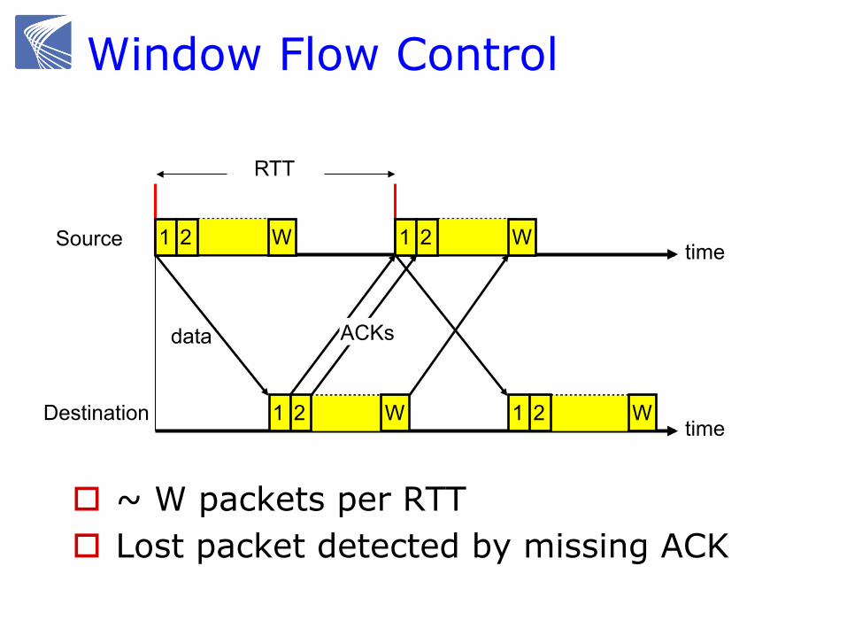
Window Flow Control
o ~ W packets per RTT o Lost packet detected by missing ACK
RTT
time
time
Source
Destination
1 2 W
1 2 W
1 2 W
data ACKs
1 2 W
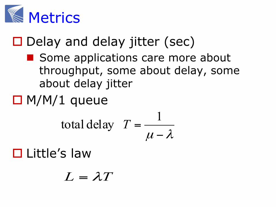
Metrics o Delay and delay jitter (sec)
n Some applications care more about throughput, some about delay, some about delay jitter
o M/M/1 queue
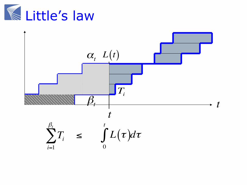
o Little’s law
λµ −=
1delay total T
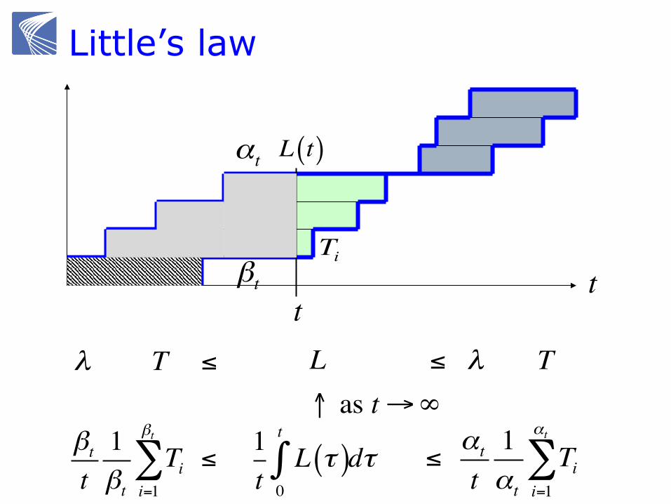
TL λ=
αt
βt
t
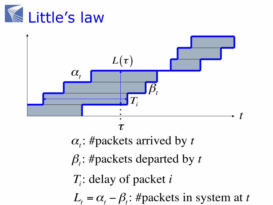
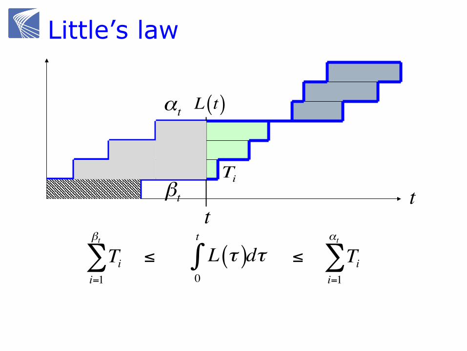
Little’s law
αt : #packets arrived by tβt : #packets departed by tTi: delay of packet iLt =αt −βt : #packets in system at t
Ti
L τ( )
τ
αt
βt t
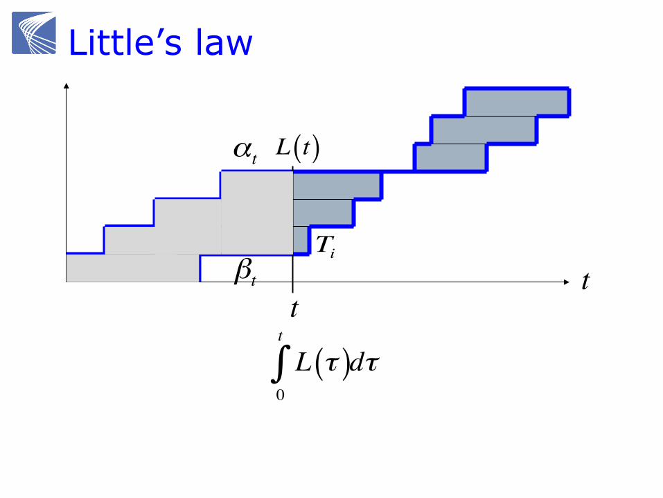
Little’s law
L τ( )0
t
∫ dτ
Ti
L t( )
t
αt
βt t
Little’s law
L τ( )0
t
∫ dτ
Ti
L t( )
t
Tii=1
βt
∑ ≤
αt
βt t
Little’s law
≤ Tii=1
αt
∑L τ( )0
t
∫ dτ
Ti
L t( )
t
Tii=1
βt
∑ ≤
αt
βt t
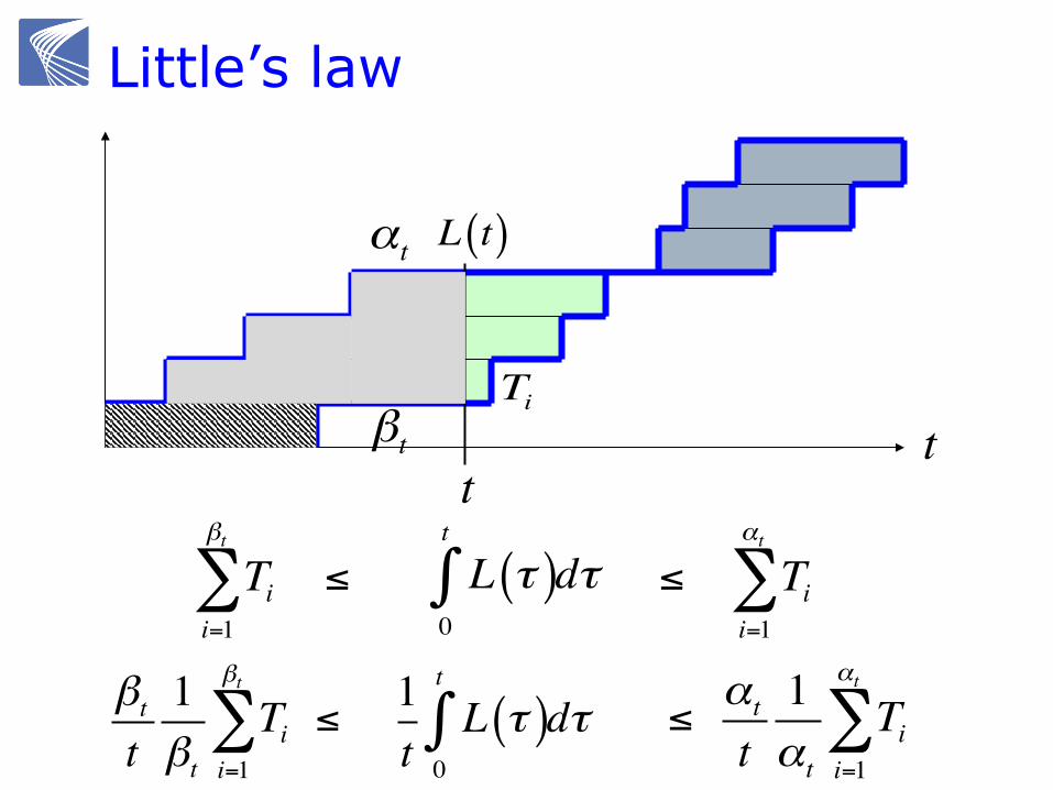
Little’s law
≤ Tii=1
αt
∑L τ( )0
t
∫ dτ
Ti
L t( )
t
Tii=1
βt
∑ ≤
1t
L τ( )0
t
∫ dτβtt
1βt
Tii=1
βt
∑ ≤ ≤ αt
t1αt
Tii=1
αt
∑
αt
βt t
Little’s law
L
Ti
L t( )
tλ T ≤
1t
L τ( )0
t
∫ dτβtt
1βt
Tii=1
βt
∑ ≤ ≤ αt
t1αt
Tii=1
αt
∑
≤ λ T↑ as t→∞
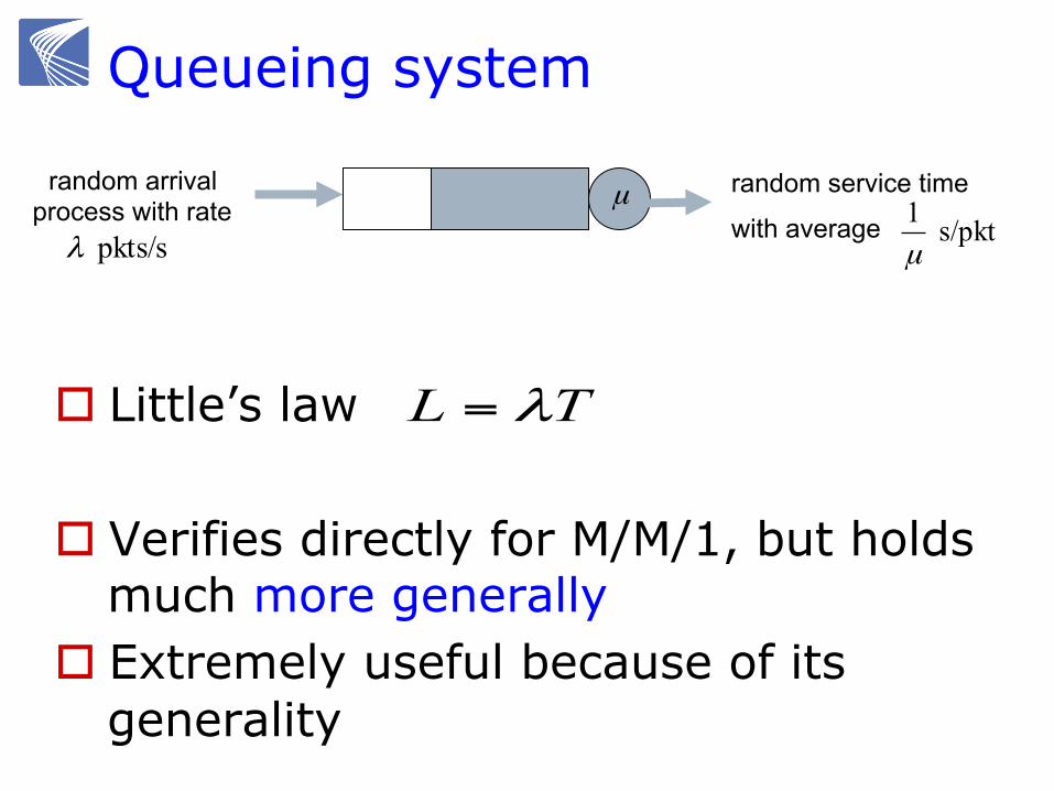
Queueing system
random arrival process with rate
pkts/s λ
random service time
with average
s/pkt 1µ
µ
o Little’s law
o Verifies directly for M/M/1, but holds much more generally
o Extremely useful because of its generality
TL λ=
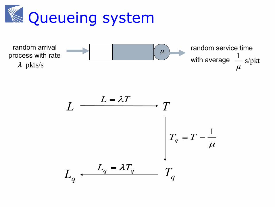
Queueing system
random arrival process with rate
pkts/s λ
random service time
with average
s/pkt 1µ
µ
T
qTqL
LTL λ=
qq TL λ=
µ1
−=TTq
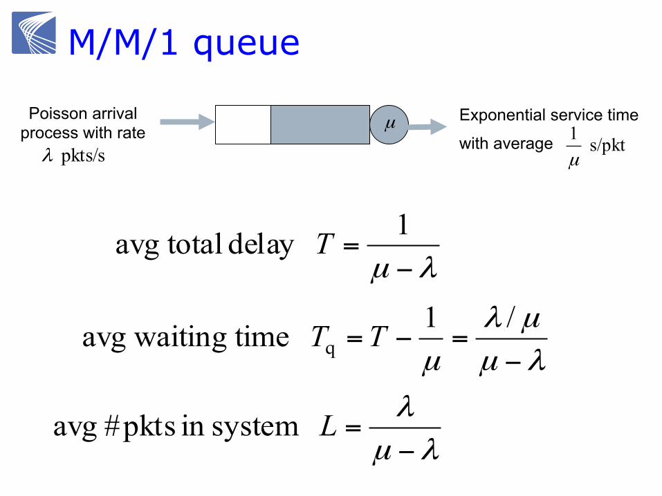
M/M/1 queue
λµλ−
=L systemin pkts# avg
Poisson arrival process with rate
pkts/s λ
Exponential service time
with average
s/pkt 1µ
µ
λµ −=
1delay totalavg T
λµµλ
µ −=−=
/1 time waitingavg q TT
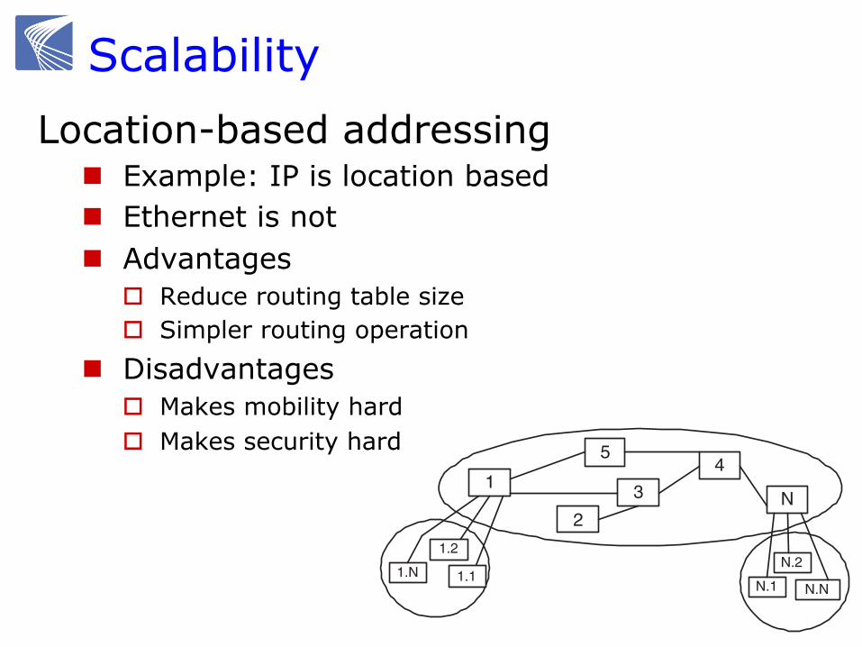
Scalability Location-based addressing
n Example: IP is location based n Ethernet is not n Advantages
o Reduce routing table size o Simpler routing operation
n Disadvantages o Makes mobility hard o Makes security hard
2.3. SCALABILITY 17
In the early days of the Internet, each computer had a complete list of all the computersattached to the network. Thus, adding one computer required updating the list that each computermaintained. Each modification had a global effect. Let us assume that half of the 1 billion computerson the Internet were added during the last ten years. That means that during these last ten yearsapproximately 0.5 × 10⁹/(10 × 365) > 105 computers were added each day, on average.
Imagine that the routers in Figure 2.1 have to store the list of all the computers that arereached to each of their ports. In that case, adding a computer to the network requires modifying alist in all the routers, clearly not a viable approach.
Consider also a scheme where the network must keep track of which computers are cur-rently exchanging information. As the network gets larger, the potential number of simultaneouscommunications also grows. Such a scheme would require increasingly complex routers.
Needless to say, it would be impossible to update all these lists to keep up with the changes.Another system had to be devised. We describe some methods that the Internet uses for scalability.
2.3.1 LOCATION-BASED ADDRESSINGWe explained in the previous chapter that the IP addresses are based on the location of the devices,in a scheme similar to the telephone numbers.
One first benefit of this approach is that it reduces the size of the routing tables, as we alreadydiscussed. Figure 2.3 shows M = N2 devices that are arranged in N groups with N devices each.Each group is attached to one router.
1
2
43 N
5
1.1
1.2
1.NN.N
N.2
N.1
Figure 2.3: A simple illustration of location-based addressing.
In this arrangement, each router 1, . . . , N needs one routing entry for each device in its groupplus one routing entry for each of the other N − 1 routers. For instance, consider a packet that goesfrom device 1.2 to device N.1. First, the packet goes from device 1.2 to router 1. Router 1 has arouting entry that specifies the next hop toward router N , say router 5. Similarly, router 5 has arouting entry for the next hop, router 4, and so on. When the packet gets to router N , the latterconsults its routing table to find the next hop toward device N.1. Thus, each routing table has sizeN + (N − 1) ≈ 2
√M .
Scalability Hierarchical
n Two level n Autonomous system
o Same administrative and/or economic domain o Shortest path routing: OSPF, IS-IS
n Inter-domain o BGP
Both simplify routing
Scalability Best effort service
n Simple TCP/IP layer
End-to-end principle n Simple network, intelligent hosts n Stateless routers
o Packet carries its own state
Both simplify router à fast big inexpensive routers
Latest (~decade) idea: software defined networking (SDN)
Scalability Hierarchical naming
n Easier on human n DNS translation
Layering n Application & technology independence
Application topology n Client/server n CDN n P2P n Cloud computing n Social networking