21.12.2009

1

1

Workflow ExampleHorn Antenna

Purpose : Optimize the

aperture of the horn

antenna such that the gain

is maximized at 10 GHz.

2

CST MWS - Standard Workflow

Choose a project template.

Create your model.

parameters + geometry + materials

Define ports.

Set the frequency range.

Specify boundary and symmetry conditions.

Define monitors.

Check the mesh.

Run the simulation.

21.12.2009

2

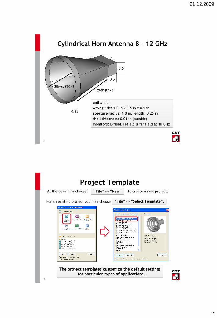
3

units: inch

waveguide: 1.0 in x 0.5 in x 0.5 in

aperture radius: 1.0 in, length: 0.25 in

shell thickness: 0.01 in (outside)

monitors: E-field, H-field & far field at 10 GHz

1

0.5

0.25

zlength=2dia=2, rad=1

0.5

Cylindrical Horn Antenna 8 – 12 GHz

4

Project TemplateAt the beginning choose to create a new project.

For an existing project you may choose

“File” -> “New”

“File” -> “Select Template”.

The project templates customize the default settings

for particular types of applications.

21.12.2009

3

5

Project Template

The project templates customize the default

settings for particular types of applications.

PEC is very practical for closed structures.

(e.g. waveguides, connectors, filters)

Antennas should be modeled with

vacuum as background material.

background material

6

Change the Units

Define units.

21.12.2009

4

7

Horn Antenna – Construction (I)

Define a brick (1.0 x 0.5 x 0.5 in)

made of PEC.

Pick face.

Align the WCS with the

face.

Move the WCS by 2.0

inches.

Define a cylinder (outer radius: 1.0 in,

height: 0.25 in) made of PEC.

8

Horn Antenna – Construction (II)

Pick two opposite faces. Perform a loft.

21.12.2009

5

9

Horn Antenna – Construction (III)

Perform a

Boolean add.

Pick two faces.

Select multiple objects

(ctrl or shift + left mouse button).

shell solid: 0.01 in

(outside)

10

Port Definition

Pick point

inside corner.

Pick edge.

Define a waveguide port.

Define the port on the internal profile.

21.12.2009

6

11

Set the Frequency Range

Set the frequency range.

12

Boundary Conditions and Symmetry Planes

21.12.2009

7

13

3D Monitors

Add field monitors for E-field, H-field, and far field at 10 GHz.

14

Mesh View (I)

mesh properties

21.12.2009

8

15

Mesh View (II)

TST at work!

16

Transient Solver: Start Simulation

The accuracy defines the steady-

state monitor.

The simulation is finished when

the electromagnetic energy in the

computational domain falls below

this level.

21.12.2009

9

17

Analyze 1D Results

energy

port signals

S-parameter

18

Analyze 2D/3D Results

port information:

• cut-off frequency

• line impedance

• propagation constant

21.12.2009

10

19

Electric Field at 10 GHz

20

Far Field at 10 GHz

21.12.2009

11

21

Polar Plot for Far Field at 10 GHz

Create a new folder “Comparison” to compare different 1D results.

phi=90 phi=0

22

Parameterization

Optimization

21.12.2009

12

23

Parameterization (I)

outer radius r1 = variable

goal: maximize gain

r1

24

Parameterization (II)

outer

radius

r1

21.12.2009

13

25

Result Processing Templates (Shift+P)

Define gain(theta) at phi=0.

1D results

Postprocessing templates provide a convenient way to calculate

derived quantities from simulation results.

Each template is evaluated for each solver run.

26

Define max of gain(theta).

0D results

Result Processing Templates (Shift+P)

Read the online help to learn more

about the postprocessing in CST MWS.

21.12.2009

14

27

Define max of gain(theta).

Result Processing Templates (Shift+P)

Alternative solution:

The maximum gain can be computed using

the “Farfield” template in “0D Results”.

28

Parameter Sweep - Settings

1

2

3

21.12.2009

15

29

The results will be automatically listed

in the “Tables” folder.

Parameter Sweep - Settings

Add a S-parameter watch.

30

Parameter Sweep – Table Results

Right click on plot

window and select

“Table Properties…”.

Choose the result curve for each

parameter value with the slider.

21.12.2009

16

31

Parameter Sweep – Table Results

parameter values

parameter values

32

Automatic Optimization

21.12.2009

17

33

Automatic Optimization

Define the parameter space.

Template based postprocessing 0D results can be

used to define very complex goal functions.

Define the goal function.

34

Automatic Optimization

Choose the “Classic Powell” optimizer. Follow the optimization.

21.12.2009

18

35

goal:

maximize gain

parameter values

1D results

Automatic Optimization - Results

36

Define a variable.

Parameterize the structure.

Define the goal function.

Set the parameter space.

Run the optimizer.

Optimization - Summary

21.12.2009

19

37

Far Field Postprocessing

terminology

broadband far field

analysis

co-/cross-polarization

phase center

tips and tricks

38

Broadband Far Field Analysis

How to plot the antenna gain for the complete

frequency range?

21.12.2009

20

39

Broadband Far Field Monitors

Create a broadband far field monitor

from the available monitors.

After monitor definition, start T-solver again!

40

Result Processing Templates (Shift+P)

Define maximum value of gain.

1D Results

21.12.2009

21

41

Broadband Far Field Monitors

far field 3D pattern

42

Broadband Far Field Monitors

21.12.2009

22

43

“Tables” -> “1D Results” -> “Broadband gain 3d”

44

Co- / Cross-Polarization

The co-polarized far field component has the same polarization

as the excitation (y-oriented in our case).

The cross-polarized far field component is orthogonal to the

co-polarized component and main lobe direction.

In order to use different polarizations for transmitting/receiving,

an antenna design goal might be to maximize the co-polarized

and minimize the cross-polarized component.

21.12.2009

23

45

polarization vector direction

(arbitrary user input possible).

If “Main lobe ... “ is not selected, the user

can enter arbitrary directions for:

-polarization plane normal (z„) (= theta axis)

-cross-polarized component (x„) (= phi axis).

1. Select the tab “Axes“.

2. Click “Main lobe/polarization

alignment“.

3. Choose the “Ludwig 3“ coordinate

system.

Co- / Cross-Polarization

46

co-polarized = Ludwig 3 vertical cross-polarized = Ludwig 3 horizontal

Co- / Cross-Polarization

21.12.2009

24

47

Co & Cross PolarizationResult Templates for Parameter Sweep and Optimization

co-polarized= Ludwig 3 vertical

cross-pol. = Ludwig 3 horizontal

48

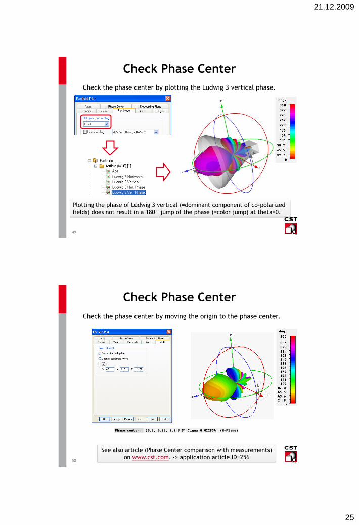
Phase Center Calculation

Finding the best location to place the horn

inside a parabolic antenna. The best position

is to match the focal point of the dish

with the phase center of the horn.

?

= x‘z‘ plane

= y‘z‘ plane

21.12.2009

25

49

Check Phase Center

Plotting the phase of Ludwig 3 vertical (=dominant component of co-polarized

fields) does not result in a 180° jump of the phase (=color jump) at theta=0.

Check the phase center by plotting the Ludwig 3 vertical phase.

50

Check Phase Center

See also article (Phase Center comparison with measurements)

on www.cst.com. -> application article ID=256

Check the phase center by moving the origin to the phase center.