Contents lists available at ScienceDirect

Computers in Biology and Medicine

journal homepage: www.elsevier.com/locate/compbiomed

CT image segmentation of bone for medical additive manufacturing using aconvolutional neural network

Jordi Minnemaa,∗, Maureen van Eijnattena,c, Wouter Kouwb, Faruk Diblenb, Adriënne Mendrikb,Jan Wolffa,d

a Amsterdam UMC and Academic Centre for Dentistry Amsterdam (ACTA), Vrije Universiteit Amsterdam, Department of Oral and Maxillofacial Surgery/Pathology, 3DInnovation Lab, Amsterdam Movement Sciences, de Boelelaan 1117, Amsterdam, the NetherlandsbNetherlands eScience Center, Science Park 140, Amsterdam, the Netherlandsc Centrum Wiskunde & Informatica (CWI), Science Park 123, Amsterdam, the Netherlandsd Department of Oral and Maxillofacial Surgery, Division for Regenerative Orofacial Medicine, University Hospital Hamburg-Eppendorf, Hamburg, Germany

A R T I C L E I N F O

Keywords:Artificial intelligenceConvolutional neural networkImage segmentationAdditive manufacturingComputed tomography (CT)

A B S T R A C T

Background: The most tedious and time-consuming task in medical additive manufacturing (AM) is imagesegmentation. The aim of the present study was to develop and train a convolutional neural network (CNN) forbone segmentation in computed tomography (CT) scans.Method: The CNN was trained with CT scans acquired using six different scanners. Standard tessellation lan-guage (STL) models of 20 patients who had previously undergone craniotomy and cranioplasty using additivelymanufactured skull implants served as “gold standard” models during CNN training. The CNN segmented allpatient CT scans using a leave-2-out scheme. All segmented CT scans were converted into STL models andgeometrically compared with the gold standard STL models.Results: The CT scans segmented using the CNN demonstrated a large overlap with the gold standard segmen-tation and resulted in a mean Dice similarity coefficient of 0.92 ± 0.04. The CNN-based STL models demon-strated mean surface deviations ranging between −0.19mm ± 0.86mm and 1.22mm ± 1.75mm, whencompared to the gold standard STL models. No major differences were observed between the mean deviations ofthe CNN-based STL models acquired using six different CT scanners.Conclusions: The fully-automated CNN was able to accurately segment the skull. CNNs thus offer the opportunityof removing the current prohibitive barriers of time and effort during CT image segmentation, making patient-specific AM constructs more accesible.

1. Introduction

Additive manufacturing (AM), also referred to as three-dimensional(3D) printing, is a technique in which successive layers of material aredeposited on a build bed, allowing the fabrication of objects withcomplex geometries [1,2]. In medicine, additive manufactured tangiblemodels are being increasingly used to evaluate complex anatomies[3,4]. Moreover, AM can be used to fabricate patient-specific constructssuch as drill guides, saw guides, and medical implants. Such constructscan markedly reduce operating times and enhance the accuracy ofsurgical procedures [4]. AM constructs have proven to be particularlyvaluable in the field of oral and maxillofacial surgery due to the ple-thora of complex bony geometries found in the skull area.

The current medical AM process comprises four different steps: 1)

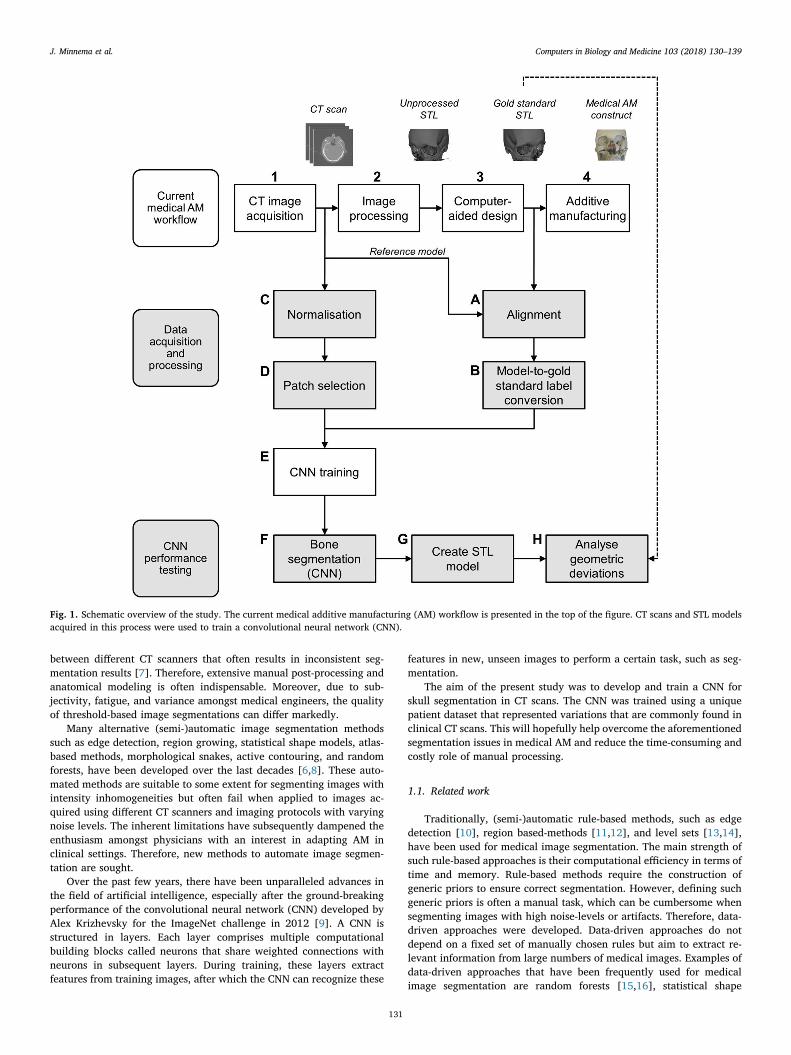
image acquisition; 2) image processing; 3) computer-aided design; and4) additive manufacturing (Fig. 1). Image acquisition is commonlyperformed using computed tomography (CT) since it offers the besthard tissue contrast [5]. During step 2 of the medical AM process, theacquired CT scan needs to be converted into a 3D surface model in thestandard tessellation language (STL) file format. This STL model can beused to design patient-specific constructs (step 3) that can subsequentlybe fabricated using a 3D printer (step 4).

The most important step in the CT-to-STL conversion process isimage segmentation: the partitioning of images into regions of interestthat correspond to a specific anatomical structure (e.g., “bone”). Todate, the most commonly used image segmentation method in medicalAM is global thresholding [6]. However, global thresholding does nottake CT artifacts and noise into account, nor the intensity variations

https://doi.org/10.1016/j.compbiomed.2018.10.012Received 7 September 2018; Received in revised form 11 October 2018; Accepted 13 October 2018

∗ Corresponding author. Amsterdam UMC, De Boelelaan 1117, 1081 HV, Amsterdam, the Netherlands.E-mail address: j.minnema@vumc.nl (J. Minnema).

Computers in Biology and Medicine 103 (2018) 130–139

0010-4825/ © 2018 Elsevier Ltd. All rights reserved.

T

between different CT scanners that often results in inconsistent seg-mentation results [7]. Therefore, extensive manual post-processing andanatomical modeling is often indispensable. Moreover, due to sub-jectivity, fatigue, and variance amongst medical engineers, the qualityof threshold-based image segmentations can differ markedly.

Many alternative (semi-)automatic image segmentation methodssuch as edge detection, region growing, statistical shape models, atlas-based methods, morphological snakes, active contouring, and randomforests, have been developed over the last decades [6,8]. These auto-mated methods are suitable to some extent for segmenting images withintensity inhomogeneities but often fail when applied to images ac-quired using different CT scanners and imaging protocols with varyingnoise levels. The inherent limitations have subsequently dampened theenthusiasm amongst physicians with an interest in adapting AM inclinical settings. Therefore, new methods to automate image segmen-tation are sought.

Over the past few years, there have been unparalleled advances inthe field of artificial intelligence, especially after the ground-breakingperformance of the convolutional neural network (CNN) developed byAlex Krizhevsky for the ImageNet challenge in 2012 [9]. A CNN isstructured in layers. Each layer comprises multiple computationalbuilding blocks called neurons that share weighted connections withneurons in subsequent layers. During training, these layers extractfeatures from training images, after which the CNN can recognize these

features in new, unseen images to perform a certain task, such as seg-mentation.

The aim of the present study was to develop and train a CNN forskull segmentation in CT scans. The CNN was trained using a uniquepatient dataset that represented variations that are commonly found inclinical CT scans. This will hopefully help overcome the aforementionedsegmentation issues in medical AM and reduce the time-consuming andcostly role of manual processing.

1.1. Related work

Traditionally, (semi-)automatic rule-based methods, such as edgedetection [10], region based-methods [11,12], and level sets [13,14],have been used for medical image segmentation. The main strength ofsuch rule-based approaches is their computational efficiency in terms oftime and memory. Rule-based methods require the construction ofgeneric priors to ensure correct segmentation. However, defining suchgeneric priors is often a manual task, which can be cumbersome whensegmenting images with high noise-levels or artifacts. Therefore, data-driven approaches were developed. Data-driven approaches do notdepend on a fixed set of manually chosen rules but aim to extract re-levant information from large numbers of medical images. Examples ofdata-driven approaches that have been frequently used for medicalimage segmentation are random forests [15,16], statistical shape

Fig. 1. Schematic overview of the study. The current medical additive manufacturing (AM) workflow is presented in the top of the figure. CT scans and STL modelsacquired in this process were used to train a convolutional neural network (CNN).

J. Minnema et al. Computers in Biology and Medicine 103 (2018) 130–139

131

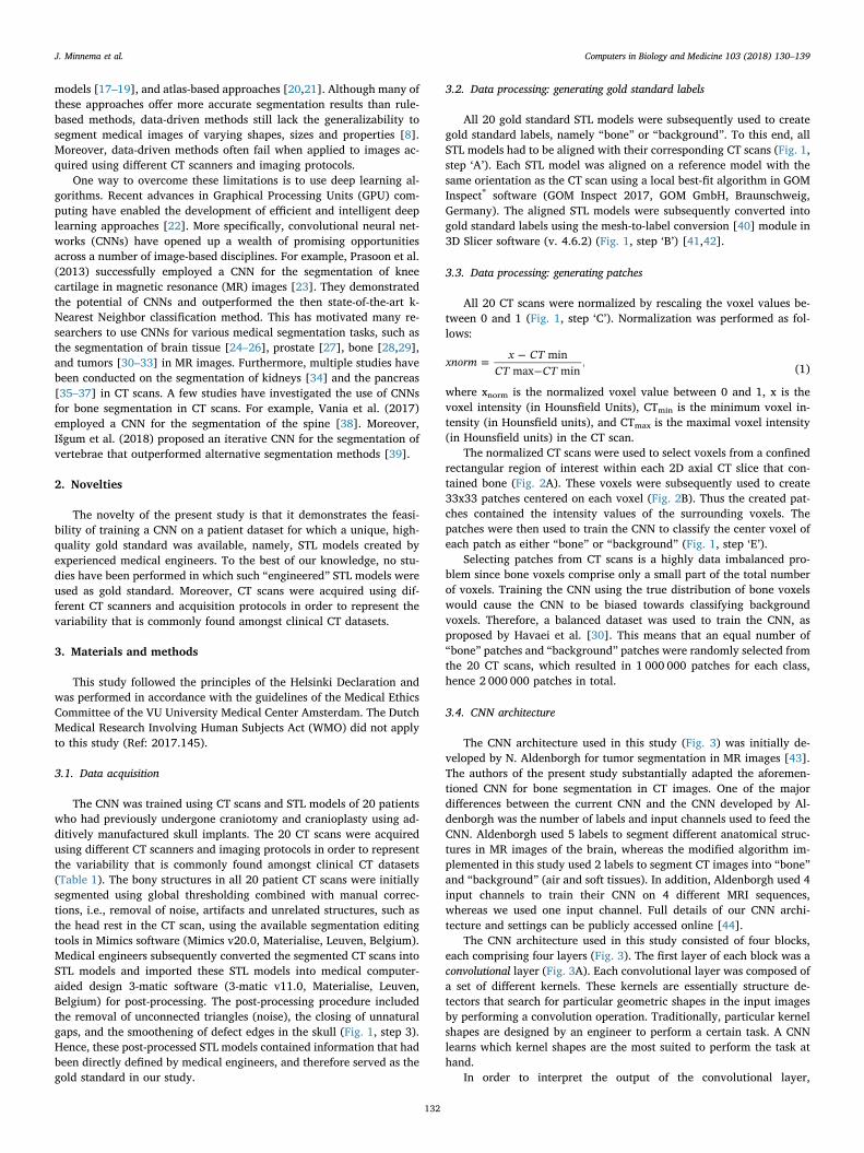
models [17–19], and atlas-based approaches [20,21]. Although many ofthese approaches offer more accurate segmentation results than rule-based methods, data-driven methods still lack the generalizability tosegment medical images of varying shapes, sizes and properties [8].Moreover, data-driven methods often fail when applied to images ac-quired using different CT scanners and imaging protocols.

One way to overcome these limitations is to use deep learning al-gorithms. Recent advances in Graphical Processing Units (GPU) com-puting have enabled the development of efficient and intelligent deeplearning approaches [22]. More specifically, convolutional neural net-works (CNNs) have opened up a wealth of promising opportunitiesacross a number of image-based disciplines. For example, Prasoon et al.(2013) successfully employed a CNN for the segmentation of kneecartilage in magnetic resonance (MR) images [23]. They demonstratedthe potential of CNNs and outperformed the then state-of-the-art k-Nearest Neighbor classification method. This has motivated many re-searchers to use CNNs for various medical segmentation tasks, such asthe segmentation of brain tissue [24–26], prostate [27], bone [28,29],and tumors [30–33] in MR images. Furthermore, multiple studies havebeen conducted on the segmentation of kidneys [34] and the pancreas[35–37] in CT scans. A few studies have investigated the use of CNNsfor bone segmentation in CT scans. For example, Vania et al. (2017)employed a CNN for the segmentation of the spine [38]. Moreover,Išgum et al. (2018) proposed an iterative CNN for the segmentation ofvertebrae that outperformed alternative segmentation methods [39].

2. Novelties

The novelty of the present study is that it demonstrates the feasi-bility of training a CNN on a patient dataset for which a unique, high-quality gold standard was available, namely, STL models created byexperienced medical engineers. To the best of our knowledge, no stu-dies have been performed in which such “engineered” STL models wereused as gold standard. Moreover, CT scans were acquired using dif-ferent CT scanners and acquisition protocols in order to represent thevariability that is commonly found amongst clinical CT datasets.

3. Materials and methods

This study followed the principles of the Helsinki Declaration andwas performed in accordance with the guidelines of the Medical EthicsCommittee of the VU University Medical Center Amsterdam. The DutchMedical Research Involving Human Subjects Act (WMO) did not applyto this study (Ref: 2017.145).

3.1. Data acquisition

The CNN was trained using CT scans and STL models of 20 patientswho had previously undergone craniotomy and cranioplasty using ad-ditively manufactured skull implants. The 20 CT scans were acquiredusing different CT scanners and imaging protocols in order to representthe variability that is commonly found amongst clinical CT datasets(Table 1). The bony structures in all 20 patient CT scans were initiallysegmented using global thresholding combined with manual correc-tions, i.e., removal of noise, artifacts and unrelated structures, such asthe head rest in the CT scan, using the available segmentation editingtools in Mimics software (Mimics v20.0, Materialise, Leuven, Belgium).Medical engineers subsequently converted the segmented CT scans intoSTL models and imported these STL models into medical computer-aided design 3-matic software (3-matic v11.0, Materialise, Leuven,Belgium) for post-processing. The post-processing procedure includedthe removal of unconnected triangles (noise), the closing of unnaturalgaps, and the smoothening of defect edges in the skull (Fig. 1, step 3).Hence, these post-processed STL models contained information that hadbeen directly defined by medical engineers, and therefore served as thegold standard in our study.

3.2. Data processing: generating gold standard labels

All 20 gold standard STL models were subsequently used to creategold standard labels, namely “bone” or “background”. To this end, allSTL models had to be aligned with their corresponding CT scans (Fig. 1,step ‘A’). Each STL model was aligned on a reference model with thesame orientation as the CT scan using a local best-fit algorithm in GOMInspect® software (GOM Inspect 2017, GOM GmbH, Braunschweig,Germany). The aligned STL models were subsequently converted intogold standard labels using the mesh-to-label conversion [40] module in3D Slicer software (v. 4.6.2) (Fig. 1, step ‘B’) [41,42].

3.3. Data processing: generating patches

All 20 CT scans were normalized by rescaling the voxel values be-tween 0 and 1 (Fig. 1, step ‘C’). Normalization was performed as fol-lows:

=−

−

xnorm x CTCT CT

minmax min

, (1)

where xnorm is the normalized voxel value between 0 and 1, x is thevoxel intensity (in Hounsfield Units), CTmin is the minimum voxel in-tensity (in Hounsfield units), and CTmax is the maximal voxel intensity(in Hounsfield units) in the CT scan.

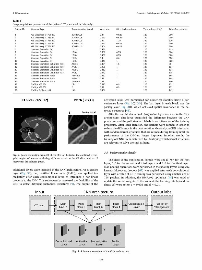
The normalized CT scans were used to select voxels from a confinedrectangular region of interest within each 2D axial CT slice that con-tained bone (Fig. 2A). These voxels were subsequently used to create33x33 patches centered on each voxel (Fig. 2B). Thus the created pat-ches contained the intensity values of the surrounding voxels. Thepatches were then used to train the CNN to classify the center voxel ofeach patch as either “bone” or “background” (Fig. 1, step ‘E’).

Selecting patches from CT scans is a highly data imbalanced pro-blem since bone voxels comprise only a small part of the total numberof voxels. Training the CNN using the true distribution of bone voxelswould cause the CNN to be biased towards classifying backgroundvoxels. Therefore, a balanced dataset was used to train the CNN, asproposed by Havaei et al. [30]. This means that an equal number of“bone” patches and “background” patches were randomly selected fromthe 20 CT scans, which resulted in 1 000 000 patches for each class,hence 2 000 000 patches in total.

3.4. CNN architecture

The CNN architecture used in this study (Fig. 3) was initially de-veloped by N. Aldenborgh for tumor segmentation in MR images [43].The authors of the present study substantially adapted the aforemen-tioned CNN for bone segmentation in CT images. One of the majordifferences between the current CNN and the CNN developed by Al-denborgh was the number of labels and input channels used to feed theCNN. Aldenborgh used 5 labels to segment different anatomical struc-tures in MR images of the brain, whereas the modified algorithm im-plemented in this study used 2 labels to segment CT images into “bone”and “background” (air and soft tissues). In addition, Aldenborgh used 4input channels to train their CNN on 4 different MRI sequences,whereas we used one input channel. Full details of our CNN archi-tecture and settings can be publicly accessed online [44].

The CNN architecture used in this study consisted of four blocks,each comprising four layers (Fig. 3). The first layer of each block was aconvolutional layer (Fig. 3A). Each convolutional layer was composed ofa set of different kernels. These kernels are essentially structure de-tectors that search for particular geometric shapes in the input imagesby performing a convolution operation. Traditionally, particular kernelshapes are designed by an engineer to perform a certain task. A CNNlearns which kernel shapes are the most suited to perform the task athand.

In order to interpret the output of the convolutional layer,

J. Minnema et al. Computers in Biology and Medicine 103 (2018) 130–139

132

additional layers were included in the CNN architecture. An activationlayer (Fig. 3B), i.e., rectified linear units (ReLU), was applied im-mediately after each convolutional layer to introduce a non-linearproperty to the CNN. This subsequently increased the flexibility of theCNN to detect different anatomical structures [9]. The output of the

activation layer was normalized for numerical stability using a nor-malization layer (Fig. 3C) [45]. The last layer in each block was thepooling layer (Fig. 3D), which achieved spatial invariance in the de-tected structures [46].

After the four blocks, a final classification layer was used in the CNNarchitecture. This layer quantified the difference between the CNNprediction and the gold standard labels in each iteration of the trainingprocedure. After each iteration, the kernels were refined in order toreduce the difference in the next iteration. Generally, a CNN is initiatedwith random kernel structures that are refined during training until theperformance of the CNN no longer improves. In other words, thetraining of CNNs is characterized by identifying which kernel structuresare relevant to solve the task at hand.

3.5. Implementation details

The sizes of the convolution kernels were set to 7x7 for the firstlayer, 5x5 for the second and third layers, and 3x3 for the final layer.Max-pooling operations were performed in the pooling layers using 2x2kernels. Moreover, dropout [47] was applied after each convolutionallayer with a value of 0.1. Training was performed using a batch size of128 patches. In addition, the RMSprop optimizer [48] was used toupdate the kernel weights. In this context, the learning rate (α) and thedecay (d) were set to α=0.005 and d= 0.01.

Table 1Image acquisition parameters of the patients’ CT scans used in this study.

Patient ID Scanner Type Reconstruction Kernel Voxel size Slice thickness (mm) Tube voltage (kVp) Tube Current (mA)

1 GE Discovery CT750 HD BONEPLUS 0.47 0.625 120 2002 GE Discovery CT750 HD BONEPLUS 0.543 0.625 120 2003 GE Discovery CT750 HD BONEPLUS 0.49 1.25 140 6264 GE Discovery CT750 HD BONEPLUS 0.553 0.625 120 2005 GE Discovery CT750 HD BONEPLUS 0.504 0.625 120 2006 Siemens Sensation 64 H31s 0.482 1 120 2137 Siemens Sensation 64 H70h 0.568 0.75 120 3008 Siemens Sensation 64 H70h 0.459 0.75 120 3009 Siemens Sensation 64 H32s 0.4 0.6 120 38010 Siemens Sensation 64 H60s 0.443 1 120 32311 Siemens Somatom Definition AS+ J30s/3 0.404 1.5 120 8012 Siemens Somatom Definition AS+ J70h/1 0.391 1 120 13113 Siemens Somatom Definition AS+ J30s/3 0.412 1 120 11314 Siemens Somatom Definition AS+ J70h/1 0.342 1 120 11515 Siemens Somatom Force Hr64h\1 0.432 1 120 18416 Siemens Somatom Force Hf38s/3 0.45 1 120 16417 Siemens Somatom Force Hr64h\1 0.39 1 120 16618 Philips iCT 256 UB 0.513 0.9 120 13119 Philips iCT 256 D 0.52 0.9 120 13120 Philips Brilliance 64 UC 0.486 1 120 149

Fig. 2. Patch acquisition from CT slices. Box A illustrates the confined rectan-gular region of interest enclosing all bone voxels in the CT slice, and box Brepresents the selected patch.

Fig. 3. Schematic overview of the CNN architecture.

J. Minnema et al. Computers in Biology and Medicine 103 (2018) 130–139

133

CNN training (Fig. 1, step ‘E’) was performed using a Linux desktopcomputer (HP Workstation Z840) with 64 GB RAM, a Xeon E5-2687 v43.0GHZ CPU, and a GTX 1080 Ti GPU card. Implementation of the codewas performed in Keras [49], a python library that compiles symbolicalexpressions into C/CUDA code that can then run on GPUs. The trainingof the CNN took approximately 5min for each epoch, while the seg-mentation of one CT slice took approximately 20 s.

3.6. CNN performance testing

The performance of the CNN was evaluated by segmenting CT scansthat were not used for training purposes (Fig. 1, step ‘F’). To this end,the CNN was trained using a leave-2-out scheme: patches were acquiredalternately from 18 of the 20 CT scans, after which the CNN was used tosegment the 2 CT scans that were not used for training. Segmentationsof the CT scans were performed by classifying each voxel individually.For this purpose, patches (33x33) were generated around each voxel inthe CT scan. These patches were subsequently forwarded through thetrained CNN, which resulted in label predictions (i.e., “bone” or“background”) of all voxels.

The quality of the CNN segmentation was evaluated using the Dicesimilarity coefficient (DSC). The definition of the DSC is given inEquation (2), where TP is the number of true positives, FP is the numberof false positives, and FN is the number of false negatives.

=

+ +

DSC TPTP FP FN

22 (2)

The TP, FP, and FN of the CNN segmentations were calculated withrespect to the gold standard labels. Since these gold standard labelswere derived from STL models that were often cropped to a specificregion of interest and thus did not always cover all bony structures inthe original CT scan, the TP, FP, and FN values were only calculatedwithin this region of interest.

All 20 CT scans segmented using the CNN were subsequently con-verted into STL models using 3D Slicer software (Fig. 1, step ‘G’). Theresulting STL models were geometrically compared with the corre-sponding gold standard STL models using the surface comparisonfunction in GOM Inspect® software. This surface comparison was per-formed on the largest connected component of the STL models andcomputes the perpendicular distance between each polygon point onthe gold standard STL model and the corresponding CNN-based STLmodel. Signed deviations between −5.0 mm and +5.0 mm weremeasured between the CNN-based STL models and the gold standardSTL models (Fig. 1, step ‘H’). The mean deviations and standard de-viations (SDs) were calculated for all CNN-based STL models of theskulls as well as for a manually selected region around the edges of eachskull defect.

4. Results

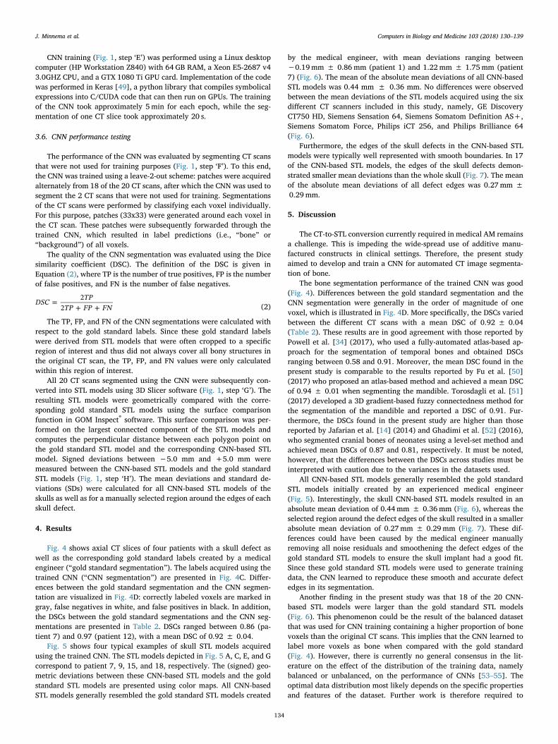
Fig. 4 shows axial CT slices of four patients with a skull defect aswell as the corresponding gold standard labels created by a medicalengineer (“gold standard segmentation”). The labels acquired using thetrained CNN (“CNN segmentation”) are presented in Fig. 4C. Differ-ences between the gold standard segmentation and the CNN segmen-tation are visualized in Fig. 4D: correctly labeled voxels are marked ingray, false negatives in white, and false positives in black. In addition,the DSCs between the gold standard segmentations and the CNN seg-mentations are presented in Table 2. DSCs ranged between 0.86 (pa-tient 7) and 0.97 (patient 12), with a mean DSC of 0.92 ± 0.04.

Fig. 5 shows four typical examples of skull STL models acquiredusing the trained CNN. The STL models depicted in Fig. 5 A, C, E, and Gcorrespond to patient 7, 9, 15, and 18, respectively. The (signed) geo-metric deviations between these CNN-based STL models and the goldstandard STL models are presented using color maps. All CNN-basedSTL models generally resembled the gold standard STL models created

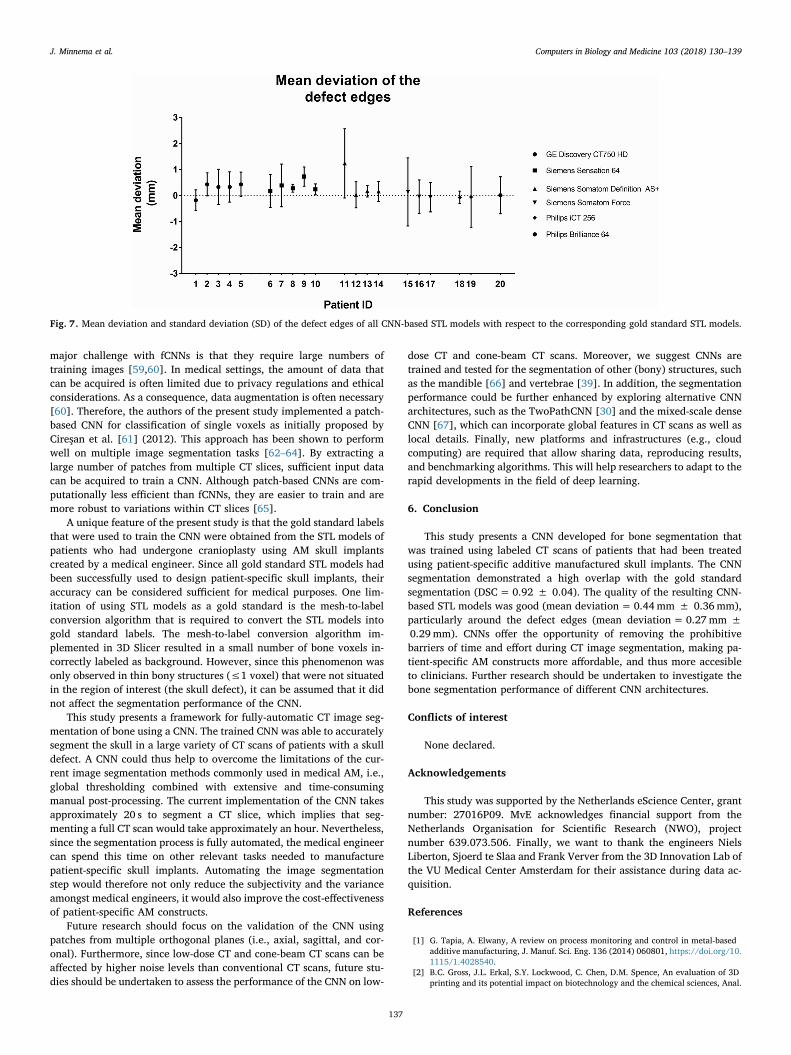
by the medical engineer, with mean deviations ranging between−0.19mm ± 0.86mm (patient 1) and 1.22mm ± 1.75mm (patient7) (Fig. 6). The mean of the absolute mean deviations of all CNN-basedSTL models was 0.44 mm ± 0.36 mm. No differences were observedbetween the mean deviations of the STL models acquired using the sixdifferent CT scanners included in this study, namely, GE DiscoveryCT750 HD, Siemens Sensation 64, Siemens Somatom Definition AS+,Siemens Somatom Force, Philips iCT 256, and Philips Brilliance 64(Fig. 6).

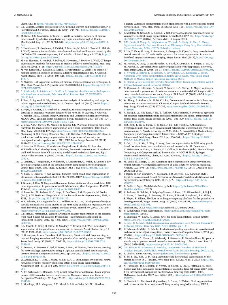
Furthermore, the edges of the skull defects in the CNN-based STLmodels were typically well represented with smooth boundaries. In 17of the CNN-based STL models, the edges of the skull defects demon-strated smaller mean deviations than the whole skull (Fig. 7). The meanof the absolute mean deviations of all defect edges was 0.27mm ±0.29mm.

5. Discussion

The CT-to-STL conversion currently required in medical AM remainsa challenge. This is impeding the wide-spread use of additive manu-factured constructs in clinical settings. Therefore, the present studyaimed to develop and train a CNN for automated CT image segmenta-tion of bone.

The bone segmentation performance of the trained CNN was good(Fig. 4). Differences between the gold standard segmentation and theCNN segmentation were generally in the order of magnitude of onevoxel, which is illustrated in Fig. 4D. More specifically, the DSCs variedbetween the different CT scans with a mean DSC of 0.92 ± 0.04(Table 2). These results are in good agreement with those reported byPowell et al. [34] (2017), who used a fully-automated atlas-based ap-proach for the segmentation of temporal bones and obtained DSCsranging between 0.58 and 0.91. Moreover, the mean DSC found in thepresent study is comparable to the results reported by Fu et al. [50](2017) who proposed an atlas-based method and achieved a mean DSCof 0.94 ± 0.01 when segmenting the mandible. Torosdagli et al. [51](2017) developed a 3D gradient-based fuzzy connectedness method forthe segmentation of the mandible and reported a DSC of 0.91. Fur-thermore, the DSCs found in the present study are higher than thosereported by Jafarian et al. [14] (2014) and Ghadimi et al. [52] (2016),who segmented cranial bones of neonates using a level-set method andachieved mean DSCs of 0.87 and 0.81, respectively. It must be noted,however, that the differences between the DSCs across studies must beinterpreted with caution due to the variances in the datasets used.

All CNN-based STL models generally resembled the gold standardSTL models initially created by an experienced medical engineer(Fig. 5). Interestingly, the skull CNN-based STL models resulted in anabsolute mean deviation of 0.44mm ± 0.36mm (Fig. 6), whereas theselected region around the defect edges of the skull resulted in a smallerabsolute mean deviation of 0.27mm ± 0.29mm (Fig. 7). These dif-ferences could have been caused by the medical engineer manuallyremoving all noise residuals and smoothening the defect edges of thegold standard STL models to ensure the skull implant had a good fit.Since these gold standard STL models were used to generate trainingdata, the CNN learned to reproduce these smooth and accurate defectedges in its segmentation.

Another finding in the present study was that 18 of the 20 CNN-based STL models were larger than the gold standard STL models(Fig. 6). This phenomenon could be the result of the balanced datasetthat was used for CNN training containing a higher proportion of bonevoxels than the original CT scans. This implies that the CNN learned tolabel more voxels as bone when compared with the gold standard(Fig. 4). However, there is currently no general consensus in the lit-erature on the effect of the distribution of the training data, namelybalanced or unbalanced, on the performance of CNNs [53–55]. Theoptimal data distribution most likely depends on the specific propertiesand features of the dataset. Further work is therefore required to

J. Minnema et al. Computers in Biology and Medicine 103 (2018) 130–139

134

establish the viability of considering the data distribution as a tunablehyperparameter that can be optimized for specific datasets. However,this would require many (cross-validated) training sessions and wouldthus be a time-consuming and computationally expensive procedure.

The mean deviations of the CNN-based STL models in this studyranged between −0.19mm ± 0.86mm and 1.22mm ± 0.39mm(Fig. 6). These results differ from those reported by Rueda et al. [56](2006), who calculated a mean geometrical distance of 1.63mm ±1.63mm using a fully-automated active appearance model for thesegmentation of cortical bone in the skull. However, the mean devia-tions found in the present study are comparable with those acquiredusing a fully-automatic atlas-based segmentation method developed bySteger et al. [20] (2012) that resulted in a mean deviation of 0.84mm.The aforementioned findings suggest that CNNs offer comparable bonesegmentation performance to the fully-automated segmentationmethods currently used in medical AM.

Another interesting finding was that the six different CT scannersused in this study did not seem to have an effect on the mean deviationsof the CNN-based STL models (Figs. 6 and 7). This indicates that theCNN was able to generalise intensity variations between different CTscanners and imaging protocols. In comparison, traditional rule-basedsegmentation methods, such as global thresholding, typically do notgeneralise well because they are based on a fixed set of features inimages, e.g., intensities. A major advantage of CNNs is that they canautomatically learn which characteristic features are relevant to seg-ment bone in multiple CT scans, which allows the CNN to segment bonein new, unseen CT scans.

Recent advances in CNN architectures for segmentation have led tothe development of fully convolutional neural networks (fCNNs)[27,57,58]. fCNNs take input images of varying sizes and produce aprobability map, rather than a classification output for a single voxel.This allows fCNNs to be trained more efficiently compared with CNNarchitectures for the classification of single voxels [57]. However, the

Fig. 4. Example of four axial CT slices of patients with a skull defect (A), the corresponding gold standard segmentation (B), the CNN segmentation (C), and thedifferences between the gold standard segmentation and the CNN segmentation (D).

Table 2Dice similarity coefficient (DSC) between the goldstandard segmentation and the CNN segmentationof all patient CT scans.

Patient ID DSC

1 0.962 0.933 0.894 0.955 0.896 0.937 0.868 0.919 0.8710 0.9411 0.8812 0.9713 0.9014 0.9615 0.9216 0.9317 0.9518 0.9619 0.9720 0.92Mean 0.92 ± 0.04

J. Minnema et al. Computers in Biology and Medicine 103 (2018) 130–139

135

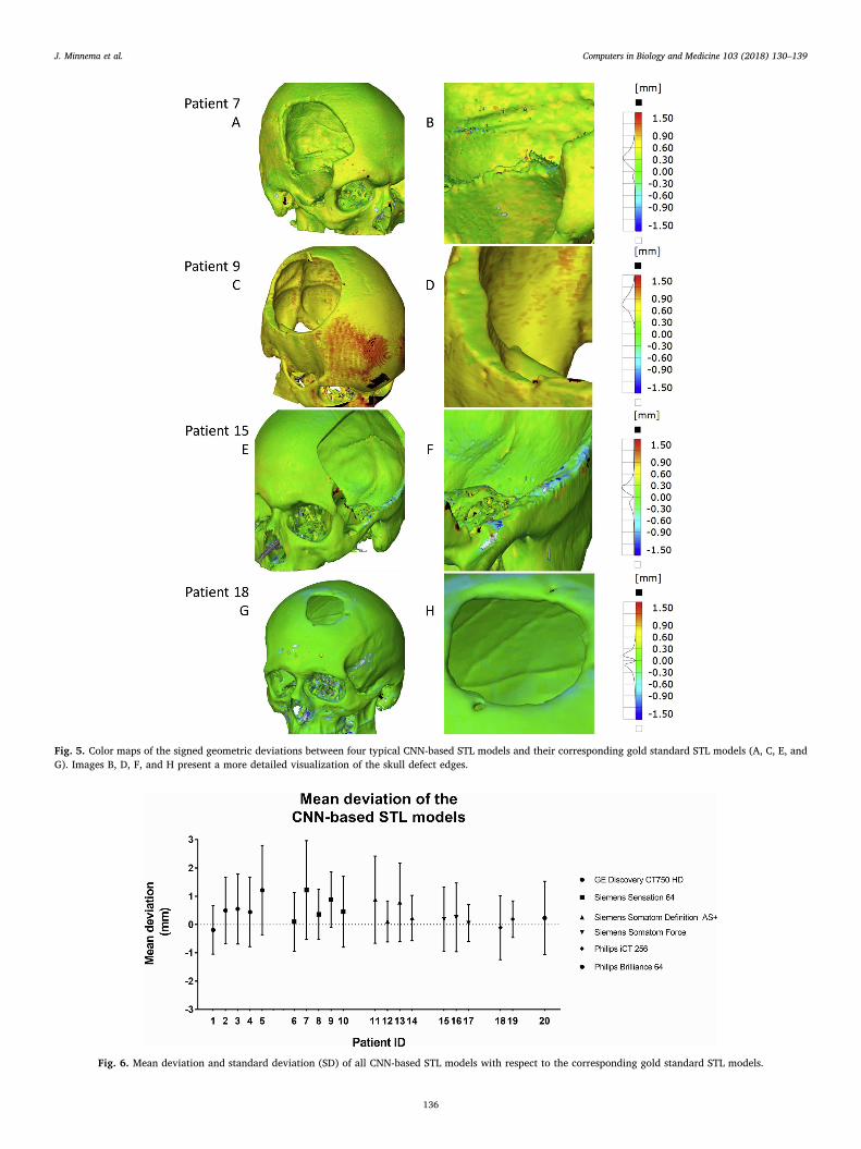
Fig. 5. Color maps of the signed geometric deviations between four typical CNN-based STL models and their corresponding gold standard STL models (A, C, E, andG). Images B, D, F, and H present a more detailed visualization of the skull defect edges.

Fig. 6. Mean deviation and standard deviation (SD) of all CNN-based STL models with respect to the corresponding gold standard STL models.

J. Minnema et al. Computers in Biology and Medicine 103 (2018) 130–139

136

major challenge with fCNNs is that they require large numbers oftraining images [59,60]. In medical settings, the amount of data thatcan be acquired is often limited due to privacy regulations and ethicalconsiderations. As a consequence, data augmentation is often necessary[60]. Therefore, the authors of the present study implemented a patch-based CNN for classification of single voxels as initially proposed byCireşan et al. [61] (2012). This approach has been shown to performwell on multiple image segmentation tasks [62–64]. By extracting alarge number of patches from multiple CT slices, sufficient input datacan be acquired to train a CNN. Although patch-based CNNs are com-putationally less efficient than fCNNs, they are easier to train and aremore robust to variations within CT slices [65].

A unique feature of the present study is that the gold standard labelsthat were used to train the CNN were obtained from the STL models ofpatients who had undergone cranioplasty using AM skull implantscreated by a medical engineer. Since all gold standard STL models hadbeen successfully used to design patient-specific skull implants, theiraccuracy can be considered sufficient for medical purposes. One lim-itation of using STL models as a gold standard is the mesh-to-labelconversion algorithm that is required to convert the STL models intogold standard labels. The mesh-to-label conversion algorithm im-plemented in 3D Slicer resulted in a small number of bone voxels in-correctly labeled as background. However, since this phenomenon wasonly observed in thin bony structures (≤1 voxel) that were not situatedin the region of interest (the skull defect), it can be assumed that it didnot affect the segmentation performance of the CNN.

This study presents a framework for fully-automatic CT image seg-mentation of bone using a CNN. The trained CNN was able to accuratelysegment the skull in a large variety of CT scans of patients with a skulldefect. A CNN could thus help to overcome the limitations of the cur-rent image segmentation methods commonly used in medical AM, i.e.,global thresholding combined with extensive and time-consumingmanual post-processing. The current implementation of the CNN takesapproximately 20 s to segment a CT slice, which implies that seg-menting a full CT scan would take approximately an hour. Nevertheless,since the segmentation process is fully automated, the medical engineercan spend this time on other relevant tasks needed to manufacturepatient-specific skull implants. Automating the image segmentationstep would therefore not only reduce the subjectivity and the varianceamongst medical engineers, it would also improve the cost-effectivenessof patient-specific AM constructs.

Future research should focus on the validation of the CNN usingpatches from multiple orthogonal planes (i.e., axial, sagittal, and cor-onal). Furthermore, since low-dose CT and cone-beam CT scans can beaffected by higher noise levels than conventional CT scans, future stu-dies should be undertaken to assess the performance of the CNN on low-

dose CT and cone-beam CT scans. Moreover, we suggest CNNs aretrained and tested for the segmentation of other (bony) structures, suchas the mandible [66] and vertebrae [39]. In addition, the segmentationperformance could be further enhanced by exploring alternative CNNarchitectures, such as the TwoPathCNN [30] and the mixed-scale denseCNN [67], which can incorporate global features in CT scans as well aslocal details. Finally, new platforms and infrastructures (e.g., cloudcomputing) are required that allow sharing data, reproducing results,and benchmarking algorithms. This will help researchers to adapt to therapid developments in the field of deep learning.

6. Conclusion

This study presents a CNN developed for bone segmentation thatwas trained using labeled CT scans of patients that had been treatedusing patient-specific additive manufactured skull implants. The CNNsegmentation demonstrated a high overlap with the gold standardsegmentation (DSC=0.92 ± 0.04). The quality of the resulting CNN-based STL models was good (mean deviation=0.44mm ± 0.36mm),particularly around the defect edges (mean deviation= 0.27mm ±0.29mm). CNNs offer the opportunity of removing the prohibitivebarriers of time and effort during CT image segmentation, making pa-tient-specific AM constructs more affordable, and thus more accesibleto clinicians. Further research should be undertaken to investigate thebone segmentation performance of different CNN architectures.

Conflicts of interest

None declared.

Acknowledgements

This study was supported by the Netherlands eScience Center, grantnumber: 27016P09. MvE acknowledges financial support from theNetherlands Organisation for Scientific Research (NWO), projectnumber 639.073.506. Finally, we want to thank the engineers NielsLiberton, Sjoerd te Slaa and Frank Verver from the 3D Innovation Lab ofthe VU Medical Center Amsterdam for their assistance during data ac-quisition.

References

[1] G. Tapia, A. Elwany, A review on process monitoring and control in metal-basedadditive manufacturing, J. Manuf. Sci. Eng. 136 (2014) 060801, https://doi.org/10.1115/1.4028540.

[2] B.C. Gross, J.L. Erkal, S.Y. Lockwood, C. Chen, D.M. Spence, An evaluation of 3Dprinting and its potential impact on biotechnology and the chemical sciences, Anal.

Fig. 7. Mean deviation and standard deviation (SD) of the defect edges of all CNN-based STL models with respect to the corresponding gold standard STL models.

J. Minnema et al. Computers in Biology and Medicine 103 (2018) 130–139

137

Chem. (2014), https://doi.org/10.1021/ac403397r.[3] C.L. Ventola, Medical applications for 3D printing: current and projected uses, P T:

Peer-Reviewed J. Formul. Manag. 39 (2014) 704–711, https://doi.org/10.1016/j.infsof.2008.09.005.

[4] M. Salmi, K.S. Paloheimo, J. Tuomi, J. Wolff, A. Mäkitie, Accuracy of medicalmodels made by additive manufacturing (rapid manufacturing), J. Cranio-Maxillofacial Surg. 41 (2013) 603–609, https://doi.org/10.1016/j.jcms.2012.11.041.

[5] E. Huotilainen, R. Jaanimets, J. Valášek, P. Marcián, M. Salmi, J. Tuomi, A. Mäkitie,J. Wolff, Inaccuracies in additive manufactured medical skull models caused by theDICOM to STL conversion process, J. Cranio-Maxillofacial Surg. 42 (2014), https://doi.org/10.1016/j.jcms.2013.10.001.

[6] M. van Eijnatten, R. van Dijk, J. Dobbe, G. Streekstra, J. Koivisto, J. Wolff, CT imagesegmentation methods for bone used in medical additive manufacturing, Med. Eng.Phys. 51 (2018) 6–16, https://doi.org/10.1016/j.medengphy.2017.10.008.

[7] M. van Eijnatten, J. Koivisto, K. Karhu, T. Forouzanfar, J. Wolff, The impact ofmanual threshold selection in medical additive manufacturing, Int. J. Comput.Assist. Radiol. Surg. 12 (2016) 607–615, https://doi.org/10.1007/s11548-016-1490-4.

[8] N. Sharma, L.M. Aggarwal, Automated medical image segmentation techniques, J.Med. Phys./Assoc. Med. Physicists India 35 (2010) 3–14, https://doi.org/10.4103/0971-6203.58777.

[9] A. Krizhevsky, I. Sutskever, H. Geoffrey E, ImageNet classification with deep con-volutional neural networks, Adv. Neural Inf. Process. Syst. 25 (NIPS2012)(2012) 1–9.

[10] J. Kaur, S. Agrawal, R. Vig, A comparative analysis of thresholding and edge de-tection segmentation techniques, Int. J. Comput. Appl. 39 (2012) 29–34, https://doi.org/10.5120/4898-7432.

[11] J. Fripp, S. Crozier, S.K. Warfield, S. Ourselin, Automatic segmentation of articularcartilage in magnetic resonance images of the knee, in: N. Ayache, S. Ourselin,A. Maeder (Eds.), Medical Image Computing and Computer-assisted Intervention –MICCAI 2007, Springer Berlin Heidelberg, Berlin, Heidelberg, 2007, pp. 186–194, ,https://doi.org/10.1007/978-3-540-75759-7_23.

[12] V. Grau, A.U.J. Mewes, M. Alcaniz, R. Kikinis, S.K. Warfield, Improved watershedtransform for medical image segmentation using prior information, IEEE Trans.Med. Imag. 23 (2004) 447–458, https://doi.org/10.1109/TMI.2004.824224.

[13] Chunming Li, Rui Huang, Zhaohua Ding, J.C. Gatenby, D.N. Metaxas, J.C. Gore, Alevel set method for image segmentation in the presence of intensity in-homogeneities with application to MRI, IEEE Trans. Image Process. 20 (2011)2007–2016, https://doi.org/10.1109/TIP.2011.2146190.

[14] N. Jafarian, K. Kazemi, H. Abrishami Moghaddam, R. Grebe, M. Fournier,M.S. Helfroush, C. Gondry-Jouet, F. Wallois, Automatic segmentation of newborns'skull and fontanel from CT data using model-based variational level set, SignalImage Video Process. 8 (2014) 377–387, https://doi.org/10.1007/s11760-012-0300-x.

[15] C. Lindner, S. Thiagarajah, J. Wilkinson, T. Consortium, G. Wallis, T. Cootes, Fullyautomatic segmentation of the proximal femur using random forest regressionvoting, IEEE Trans. Med. Imag. 32 (2013) 1462–1472, https://doi.org/10.1109/TMI.2013.2258030.

[16] N. Baka, S. Leenstra, T. van Walsum, Random forest-based bone segmentation inultrasound, Ultrasound Med. Biol. 43 (2017) 2426–2437, https://doi.org/10.1016/j.ultrasmedbio.2017.04.022.

[17] J. Schmid, J. Kim, N. Magnenat-Thalmann, Robust statistical shape models for MRIbone segmentation in presence of small field of view, Med. Image Anal. 15 (2011)155–168, https://doi.org/10.1016/j.media.2010.09.001.

[18] H. Lamecker, M. Seebass, H.-C. Hege, P. Deuflhard, J.M. Fitzpatrick, M. Sonka(Eds.), A 3D Statistical Shape Model of the Pelvic Bone for Segmentation, 2004, p.1341, , https://doi.org/10.1117/12.534145.

[19] M.A. Baldwin, J.E. Langenderfer, P.J. Rullkoetter, P.J. Laz, Development of subject-specific and statistical shape models of the knee using an efficient segmentation andmesh-morphing approach, Comput. Methods Progr. Biomed. 97 (2010) 232–240,https://doi.org/10.1016/j.cmpb.2009.07.005.

[20] S. Steger, M. Kirschner, S. Wesarg, Articulated atlas for segmentation of the skeletonfrom head & neck CT datasets, Proceedings - International Symposium onBiomedical Imaging, 2012, pp. 1256–1259, , https://doi.org/10.1109/ISBI.2012.6235790.

[21] K.A. Powell, T. Liang, B. Hittle, D. Stredney, T. Kerwin, G.J. Wiet, Atlas-basedsegmentation of temporal bone anatomy, Int. J. Comput. Assist. Radiol. Surg. 12(2017) 1937–1944, https://doi.org/10.1007/s11548-017-1658-6.

[22] H. Greenspan, B. van Ginneken, R.M. Summers, Guest editorial deep learning inmedical imaging: overview and future promise of an exciting new technique, IEEETrans. Med. Imag. 35 (2016) 1153–1159, https://doi.org/10.1109/TMI.2016.2553401.

[23] A. Prasoon, K. Petersen, C. Igel, F. Lauze, E. Dam, M. Nielsen, Deep feature learningfor knee cartilage segmentation using a triplanar convolutional neural network,Lecture Notes in Computer Science, 2013, pp. 246–253, , https://doi.org/10.1007/978-3-642-40763-5_31.

[24] W. Zhang, R. Li, H. Deng, L. Wang, W. Lin, S. Ji, D. Shen, Deep convolutional neuralnetworks for multi-modality isointense infant brain image segmentation,Neuroimage 108 (2015) 214–224, https://doi.org/10.1016/j.neuroimage.2014.12.061.

[25] A. De Brébisson, G. Montana, Deep neural networks for anatomical brain segmen-tation, IEEE Computer Society Conference on Computer Vision and PatternRecognition Workshops, 2015, pp. 20–28, , https://doi.org/10.1109/CVPRW.2015.7301312.

[26] P. Moeskops, M.A. Viergever, A.M. Mendrik, L.S. de Vries, M.J.N.L. Benders,

I. Isgum, Automatic segmentation of MR brain images with a convolutional neuralnetwork, IEEE Trans. Med. Imag. 35 (2016) 1252–1261, https://doi.org/10.1109/TMI.2016.2548501.

[27] F. Milletari, N. Navab, S.-A. Ahmadi, V-Net, Fully convolutional neural networks forvolumetric medical image segmentation, ArXiv:1606.04797 [Cs] http://arxiv.org/abs/1606.04797, (2016) , Accessed date: 17 August 2018.

[28] C.M. Deniz, S. Xiang, S. Hallyburton, A. Welbeck, S. Honig, K. Cho, G. Chang,Segmentation of the Proximal Femur from MR Images Using Deep ConvolutionalNeural Networks, ArXiv, (2017) (Published online).

[29] F. Liu, Z. Zhou, H. Jang, A. Samsonov, Z. Gengyan, R. Kijowski, Deep convolutionalneural network and 3D deformable approach for tissue segmentation in muscu-loskeletal magnetic resonance imaging, Magn. Reson. Med. (2017), https://doi.org/10.1002/mrm.26841.

[30] M. Havaei, A. Davy, D. Warde-Farley, A. Biard, A. Courville, Y. Bengio, C. Pal, P.-M. Jodoin, H. Larochelle, Brain tumor segmentation with deep neural networks,Med. Image Anal. 35 (2016) 18–31, https://doi.org/10.1016/j.media.2016.05.004.

[31] R. Vivanti, A. Ephrat, L. Joskowicz, N. Lev-Cohain, O.A. Karaaslan, J. Sosna,Automatic liver tumor segmentation in follow-up CT scans, Proc. Patch-basedMethods in Medical Image Processing Workshop, 2015.

[32] C. Elamri, A New Algorithm for Fully Automatic Brain Tumor Segmentation with 3-D Convolutional Neural Networks, (2016).

[33] O. Charron, A. Lallement, D. Jarnet, V. Noblet, J.-B. Clavier, P. Meyer, Automaticdetection and segmentation of brain metastases on multimodal MR images with adeep convolutional neural network, Comput. Biol. Med. 95 (2018) 43–54, https://doi.org/10.1016/j.compbiomed.2018.02.004.

[34] W. Thong, S. Kadoury, N. Piché, C.J. Pal, Convolutional networks for kidney seg-mentation in contrast-enhanced CT scans, Comput. Methods Biomech. Biomed.Eng.: Imag. Visual. 6 (2018) 277–282, https://doi.org/10.1080/21681163.2016.1148636.

[35] A. Farag, L. Lu, H.R. Roth, J. Liu, E. Turkbey, R.M. Summers, A bottom-up approachfor pancreas segmentation using cascaded superpixels and (deep) image patch la-beling, IEEE Trans. Image Process. 26 (2017) 386–399, https://doi.org/10.1109/TIP.2016.2624198.

[36] H.R. Roth, L. Lu, A. Farag, H.-C. Shin, J. Liu, E.B. Turkbey, R.M. Summers,DeepOrgan: multi-level deep convolutional networks for automated pancreas seg-mentation, in: N. Navab, J. Hornegger, W.M. Wells, A. Frangi (Eds.), Medical ImageComputing and Computer-assisted Intervention – MICCAI 2015, SpringerInternational Publishing, Cham, 2015, pp. 556–564, , https://doi.org/10.1007/978-3-319-24553-9_68.

[37] J. Cai, L. Lu, Y. Xie, F. Xing, L. Yang, Pancreas segmentation in MRI using graph-based decision fusion on convolutional neural networks, in: M. Descoteaux,L. Maier-Hein, A. Franz, P. Jannin, D.L. Collins, S. Duchesne (Eds.), Medical ImageComputing and Computer-assisted Intervention − MICCAI 2017, SpringerInternational Publishing, Cham, 2017, pp. 674–682, , https://doi.org/10.1007/978-3-319-66179-7_77.

[38] M. Vania, D. Mureja, D. Lee, Automatic spine segmentation using convolutionalneural network via redundant generation of class labels for 3D spine modeling,ArXiv:1712.01640 [Cs] http://arxiv.org/abs/1712.01640, (2017) , Accessed date:20 August 2018.

[39] I. Išgum, B. van Ginneken, N. Lessmann, E.D. Angelini, B.A. Landman (Eds.),Iterative Convolutional Neural Networks for Automatic Vertebra Identification andSegmentation in CT Images, SPIE, 2018, p. 7, , https://doi.org/10.1117/12.2292731.

[40] F. Budin, I. Oguz, MeshToLabelMap, github, https://github.com/NIRALUser/MeshToLabelMap, (2017).

[41] A. Fedorov, R. Beichel, J. Kalpathy-Cramer, J. Finet, J.C. Fillion-Robin, S. Pujol,C. Bauer, D. Jennings, F. Fennessy, M. Sonka, J. Buatti, S. Aylward, J.V. Miller,S. Pieper, R. Kikinis, 3D slicer as an image computing platform for the quantitativeimaging network, Magn. Reson. Imag. 30 (2012) 1323–1341, https://doi.org/10.1016/j.mri.2012.05.001.

[42] 3DSlicer.org, (n.d.). www.slicer.org (Accessed 23 January 2018).[43] N. Aldenborgh, brain_segmentation, https://github.com/naldeborgh7575/brain_

segmentation, (2016).[44] J. Minnema, W. Kouw, F. Diblen, CNN for bone segmentation, Github (2018),

https://doi.org/10.5281/zenodo.1164605.[45] S. Ioffe, C. Szegedy, Batch Normalization: Accelerating Deep Network Training by

Reducing Internal Covariate Shift, Arxiv, (2015), pp. 1–11.[46] D. Scherer, A. Müller, S. Behnke, Evaluation of pooling operations in convolutional

architectures for object recognition, Lecture Notes in Computer Science, 2010, pp.92–101, , https://doi.org/10.1007/978-3-642-15825-4_10.

[47] N. Srivastava, G. Hinton, A. Krizhevsky, I. Sutskever, R. Salakhutdinov, Dropout: asimple way to prevent neural networks from overfitting, J. Mach. Learn. Res. 15(2014) 1929–1958, https://doi.org/10.1214/12-AOS1000.

[48] G.E. Hinton, N. Srivastava, K. Swersky, Lecture 6a- Overview of Mini-batchGradient Descent, COURSERA: Neural Networks for Machine Learning, 2012, p. 31.

[49] F. Chollet, Keras, GitHub, https://github.com/fchollet/keras, (2015).[50] Y. Fu, S. Liu, H.H. Li, D. Yang, Automatic and hierarchical segmentation of the

human skeleton in CT images, Phys. Med. Biol. 62 (2017) 2812–2833, https://doi.org/10.1088/1361-6560/aa6055.

[51] N. Torosdagli, D.K. Liberton, P. Verma, M. Sincan, J. Lee, S. Pattanaik, U. Bagci,Robust and fully automated segmentation of mandible from CT scans, 2017 IEEE14th International Symposium on Biomedical Imaging (ISBI 2017), IEEE,Melbourne, Australia, 2017, pp. 1209–1212, , https://doi.org/10.1109/ISBI.2017.7950734.

[52] S. Ghadimi, H. Abrishami Moghaddam, R. Grebe, F. Wallois, Skull segmentationand reconstruction from newborn CT images using coupled level sets, IEEE J.

J. Minnema et al. Computers in Biology and Medicine 103 (2018) 130–139

138

Biomed. Health Inform. 20 (2016) 563–573, https://doi.org/10.1109/JBHI.2015.2391991.

[53] F. Provost, G.M. Weiss, Learning when Training Data Are Costly: the Effect of ClassDistribution on Tree Induction, (2011), https://doi.org/10.1613/jair.1199ArXiv:1106.4557 [Cs].

[54] Haibo He, E.A. Garcia, Learning from imbalanced data, IEEE Trans. Knowl. DataEng. 21 (2009) 1263–1284, https://doi.org/10.1109/TKDE.2008.239.

[55] G.E.A.P.A. Batista, R.C. Prati, M.C. Monard, A study of the behavior of severalmethods for balancing machine learning training data, ACM SIGKDD ExplorationsNewsletter - Special Issue on Learning from Imbalanced Datasets, vol 6, 2004, pp.20–29, , https://doi.org/10.1145/1007730.1007735.

[56] S. Rueda, J.A. Gil, R. Pichery, M. Alcañiz, Automatic segmentation of jaw tissues inCT using active appearance models and semi-automatic landmarking., MedicalImage Computing and Computer-Assisted Intervention : MICCAI, InternationalConference on Medical Image Computing and Computer-assisted Intervention, vol.9, 2006, pp. 167–174, , https://doi.org/10.1007/11866565_21.

[57] J. Long, E. Shelhamer, T. Darrell, Fully convolutional networks for semantic seg-mentation, ArXiv:1411.4038 [Cs] http://arxiv.org/abs/1411.4038, (2014) ,Accessed date: 20 August 2018.

[58] O. Ronneberger, P. Fischer, T. Brox, U-net: convolutional networks for biomedicalimage segmentation, Medical Image Computing and Computer-assistedIntervention – MICCAI 2015, 2015, pp. 234–241, , https://doi.org/10.1007/978-3-319-24574-4_28.

[59] J. Bernal, K. Kushibar, M. Cabezas, S. Valverde, A. Oliver, X. Lladó, Quantitativeanalysis of patch-based fully convolutional neural networks for tissue segmentationon brain magnetic resonance imaging, ArXiv:1801.06457 [Cs] http://arxiv.org/abs/1801.06457, (2018) , Accessed date: 20 August 2018.

[60] B. Kayalibay, G. Jensen, P. van der Smagt, CNN-based segmentation of medical

imaging data, ArXiv:1701.03056 [Cs] http://arxiv.org/abs/1701.03056, (2017) ,Accessed date: 20 August 2018.

[61] D. Ciresan, A. Giusti, L.M. Gambardella, J. Schmidhuber, Deep neural networkssegment neuronal membranes in electron microscopy images, in: F. Pereira,C.J.C. Burges, L. Bottou, K.Q. Weinberger (Eds.), Advances in Neural InformationProcessing Systems, vol 25, Curran Associates, Inc., 2012, pp. 2843–2851 http://papers.nips.cc/paper/4741-deep-neural-networks-segment-neuronal-membranes-in-electron-microscopy-images.pdf.

[62] S. Pereira, A. Pinto, V. Alves, C.A. Silva, Brain tumor segmentation using con-volutional neural networks in MRI images, IEEE Trans. Med. Imag. 35 (2016)1240–1251, https://doi.org/10.1109/TMI.2016.2538465.

[63] C. Wachinger, M. Reuter, T. Klein, DeepNAT: deep convolutional neural network forsegmenting neuroanatomy, Neuroimage 170 (2018) 434–445, https://doi.org/10.1016/j.neuroimage.2017.02.035.

[64] S. Trebeschi, J.J.M. van Griethuysen, D.M.J. Lambregts, M.J. Lahaye, C. Parmar,F.C.H. Bakers, N.H.G.M. Peters, R.G.H. Beets-Tan, H.J.W.L. Aerts, Deep learning forfully-automated localization and segmentation of rectal cancer on multiparametricMR, Sci. Rep. 7 (2017), https://doi.org/10.1038/s41598-017-05728-9.

[65] L. Hou, D. Samaras, T.M. Kurc, Y. Gao, J.E. Davis, J.H. Saltz, Patch-based con-volutional neural network for whole slide tissue image classification, 2016 IEEEConference on Computer Vision and Pattern Recognition (CVPR), IEEE, Las Vegas,NV, USA, 2016, pp. 2424–2433, , https://doi.org/10.1109/CVPR.2016.266.

[66] B. Qiu, J. Guo, J. Kraeima, R. Borra, M. Witjes, P. van Ooijen, 3D Segmentation ofMandible from Multisectional CT Scans by Convolutional Neural Networks,OpenReview.Net., 2018.

[67] D.M. Pelt, J.A. Sethian, A mixed-scale dense convolutional neural network forimage analysis, Proc. Natl. Acad. Sci. Unit. States Am. 115 (2018) 254–259, https://doi.org/10.1073/pnas.1715832114.

J. Minnema et al. Computers in Biology and Medicine 103 (2018) 130–139

139