Embed Size (px)
Citation preview


Copyright Dr Robert Mitchell 2010
2 Surviving Maths in AS Biology
CT Publications
Surviving Maths
in AS Biology by
Dr Robert Mitchell
www.SurvivingMathsInASBiology.co.uk

Copyright Dr Robert Mitchell 2010
3 Dr Robert Mitchell
A catalogue record for this book is available from the British Library
ISBN 978-1-907769-07-8
First published in September 2010 by
CT Publications
Copyright © Dr Robert Mitchell 2010
The right of Robert Mitchell to be identified as the author of this work has been asserted by him
in accordance with the Copyright and Designs and Patents Act 1988. All rights reserved. No
part of this publication may be reproduced or transmitted in any form or by any means,
electronic or mechanical, including photocopy, recording or any information storage and
retrieval system, without permission in writing from the publisher at the address below.
Published by
CT Publications*
40 Higher Bridge Street
Bolton
Greater Manchester
BL1 2HA
First printing September 2010
10 9 8 7 6 5 4 3 2 1
*CT Publications is owned by Chemistry Tutorials located at the same address.

Copyright Dr Robert Mitchell 2010
4 Surviving Maths in AS Biology
Contents Contents .............................................................................................................................................. 4
Acknowledgements ............................................................................................................................. 6
About the author ................................................................................................................................ 6
Other books by the author ................................................................................................................. 6
Preface ................................................................................................................................................ 7
Student resources ............................................................................................................................... 8
How to use this book .......................................................................................................................... 9
Section 1: Mathematical Requirements ............................................................................................... 10
Arithmetical and numerical computation ......................................................................................... 12
Selecting the right calculator ........................................................................................................ 12
Fractions, ratios, percentages and Stuff ....................................................................................... 12
Handling Data .................................................................................................................................... 15
Rounding ....................................................................................................................................... 15
Significant figures .......................................................................................................................... 16
Graphs ............................................................................................................................................... 17
Plotting graphs .............................................................................................................................. 17
Linear relationships ....................................................................................................................... 17
Frequency tables, pie charts, bar charts and histograms ............................................................. 20
Scatter diagrams ........................................................................................................................... 22
Algebra .............................................................................................................................................. 24
Symbols ......................................................................................................................................... 24
Rearranging equations .................................................................................................................. 24
Conversion of Units ....................................................................................................................... 27
Geometry .......................................................................................................................................... 29
Two dimensional objects .............................................................................................................. 29
Three dimensional objects ............................................................................................................ 29
How science works ............................................................................................................................ 32
Types of data ................................................................................................................................. 33
Types of variable ........................................................................................................................... 33
Data quality ................................................................................................................................... 34
Errors ............................................................................................................................................. 35
Sampling ........................................................................................................................................ 36
Data analysis ................................................................................................................................. 37

Copyright Dr Robert Mitchell 2010
5 Dr Robert Mitchell
Statistical analysis ......................................................................................................................... 40
Probability ..................................................................................................................................... 40
End of Section 1 Test ......................................................................................................................... 42
End of Section 1 Test Answers .......................................................................................................... 47
Section 2:............................................................................................................................................... 52
Calculations in AS Biology Specifications .............................................................................................. 52
The art of reading questions ............................................................................................................. 53
Magnification questions ................................................................................................................... 54
Magnification and actual size ....................................................................................................... 54
Actual size using a scale bar .......................................................................................................... 55
Heart, breathing and cycle rates ....................................................................................................... 56
Osmosis ............................................................................................................................................. 58
Ѱcell = Ѱs + Ѱp ................................................................................................................................ 59
Experimental determination of water potential ........................................................................... 59
Nucleotide bases in DNA/RNA .......................................................................................................... 61
Number of bases on DNA and amino acids in proteins ................................................................ 61
Ratios of A:T, C:G .......................................................................................................................... 62
Index of diversity ............................................................................................................................... 63
Data handling and interpretation ..................................................................................................... 64
Describing lines ............................................................................................................................. 64
Comparing lines ............................................................................................................................ 66
Data manipulation ........................................................................................................................ 66
Causation and correlation ............................................................................................................. 69
End of Section 2 Test ......................................................................................................................... 70
Section 3: Examination-style Questions ............................................................................................... 80
Multi-choice questions ..................................................................................................................... 94
Section 4: Answers to the Exam Questions .......................................................................................... 96
Answers to examination-style questions .......................................................................................... 97
Glossary of HSW terms ................................................................................................................... 105
Index................................................................................................................................................ 106
Other books by CT Publications ...................................................................................................... 107

Copyright Dr Robert Mitchell 2010
6 Surviving Maths in AS Biology
Acknowledgements
I would like to thank Denise for her infinite patience, her reading and proofing
skills and having the unending ability to encourage and support the production of
this work. Thanks also to my Mum, Joyce and Brother, Colin for just being there.
About the author
Rob is a private tutor in chemistry and biology in Bolton. He’s formerly worked in
medical research as technician, research assistant and post-doctoral researcher
and has contributed to the publication of over 40 research papers. During a
varied career in science, he’s been a project leader in industry, a lecturer and
examiner and blogs daily as Chemicalguy. He likes dogs, and pies, going to the
movies and walking!
Other books by the author
AQA A2 Biology; Writing the Synoptic Essay May 2010
Surviving Maths in AS Chemistry August 2010
Ultimate Exam Preparation; AQA Chemistry Unit 1 October 2010 (in press)
Ultimate Exam Preparation; AQA Biology Unit 1 November 2010 (in press)
Biofuelishness (Popular Science) December 2010 (in press)

Copyright Dr Robert Mitchell 2010
7 Dr Robert Mitchell
Preface
Love it or hate it, you can't escape from doing maths in biology A-level. Since the
introduction of the new-style specifications in 2008, the exam papers have
included between 10 - 30% calculation and mathematical transformations. In the
ISA or EMPA parts of the specifications this can increase to almost 50%. This
means that those of you wanting to secure the grade A, or A* qualifications will be
unlikely to achieve it without mastering the mathematical principles.
All exam boards publish the same set of Mathematical Requirements. While these
are a basic set of criteria, I have found over the years that students often
struggle with these concepts to the point that they can impact severely on the
outcome in their exams. Part of the reason for this is that students often do not
link and carry forwards some of the material from the GCSE. Even when they do,
being able to calculate proportions in a GCSE maths class, for example is not
necessarily an indicator of them being able to apply proportional changes into an
investigation into enzyme activity in A-level biology.
This book aims to put this right! It is split into four main sections. Section 1
covers the basic mathematical requirements outlined in the specifications using
examples from the AS biology syllabus. Section 2 then systematically covers all
the AS mathematical content of the biology courses giving you simple and robust
techniques for getting these calculations right every time! Section 3 will then give
you many examples of exam-style questions using the styling from AQA, Edexcel,
OCR and WJEC. These of course come with mark schemes and a breakdown of the
points so you can see how they are awarded in Section 4.
As with all the books from CT Publications the emphasis is on showing you how to do
the content and get the exam points rather than helping you understand why you
are doing it. I wish you the very best of luck to you all in your exams and future
careers.
Dr Robert Mitchell
Summer 2010

Copyright Dr Robert Mitchell 2010
8 Surviving Maths in AS Biology
Student resources
I publish two regular blogs covering various aspects of studying A-level chemistry
and biology. All updates on new products and services are posted on these blogs
before any other announcements. They are found at:
www.chemicalguy.wordpress.com [chemistry]
www.howscienceworks.wordpress.com [biology]
Pop along to this book’s dedicated website for some more exam questions and
worked examples.
www.SurvivingMathsInASBiology.co.uk
I also recommend using www.thestudentroom.co.uk for free help and support.

Copyright Dr Robert Mitchell 2010
9 Dr Robert Mitchell
How to use this book
Also consider: 1. Lose the book 2. Buy it again 3. Write an excellent review on
Amazon.co.uk or CTPublucations.co.uk, and 4. Recommend the book to all your
classmates, teachers, head of science and college library book-buying officer. ☺
So many books show you what you need to know but miss out the obvious! How to
do it! You should assume you know nothing and read through the entire book. You’ll
find an End of Section Test at ... errm the end of each section which you should
complete before attempting the exam questions. Always, always, always monitor
your performance and be critical of your own answers when marking your efforts.
If you always work on fixing the weaker areas you will gain the most improvement
in the least time!
You will also notice the placed strategically throughout. This symbol infers
that those points are common mistakes you must be aware of and avoid.
The terms sig fig and dp refer to the number of significant figures and decimal
places respectively that a number is rounded to.

Copyright Dr Robert Mitchell 2010
10 Surviving Maths in AS Biology
Section 1: Mathematical Requirements
All exam boards publish a similar set of mathematical criteria. These are a series
of statements that identify what you should be able to understand, or do, on
entry into the AS level. Most of it might be the stuff you’d prefer to forget, or
prefer not to remember that you never knew how to do it in the first place! Work
through the following material even if you don’t like it, you’ll be glad you did later.
I’ve also included a section on the How Science Works aspects which will be
expanded on later in Section 2 and 3.
Copyright Dr Robert Mitchell 2010
11 Dr Robert Mitchell
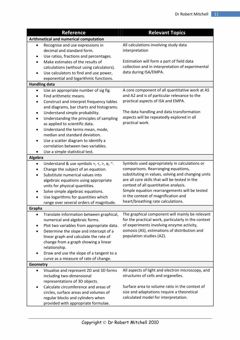
Reference Relevant Topics Arithmetical and numerical computation
Recognise and use expressions in decimal and standard form.
Use ratios, fractions and percentages.
Make estimates of the results of calculations (without using calculators).
Use calculators to find and use power, exponential and logarithmic functions.
All calculations involving study data interpretation Estimation will form a part of field data collection and in interpretation of experimental data during ISA/EMPA.
Handling data
Use an appropriate number of sig fig.
Find arithmetic means.
Construct and interpret frequency tables and diagrams, bar charts and histograms.
Understand simple probability.
Understanding the principles of sampling as applied to scientific data.
Understand the terms mean, mode, median and standard deviation.
Use a scatter diagram to identify a correlation between two variables.
Use a simple statistical test.
A core component of all quantitative work at AS and A2 and is of particular relevance to the practical aspects of ISA and EMPA. The data handling and data transformation aspects will be repeatedly explored in all practical work.
Algebra
Understand & use symbols =, <, >, α, ~.
Change the subject of an equation.
Substitute numerical values into algebraic equations using appropriate units for physical quantities.
Solve simple algebraic equations.
Use logarithms for quantities which range over several orders of magnitude.
Symbols used appropriately in calculations or comparisons. Rearranging equations, substituting in values, solving and changing units are all core skills that will be tested in the context of all quantitative analysis. Simple equation rearrangements will be tested in the context of magnification and heart/breathing rate calculations.
Graphs
Translate information between graphical, numerical and algebraic forms.
Plot two variables from appropriate data.
Determine the slope and intercept of a linear graph and calculate the rate of change from a graph showing a linear relationship.
Draw and use the slope of a tangent to a curve as a measure of rate of change.
The graphical component will mainly be relevant for the practical work, particularly in the context of experiments involving enzyme activity, osmosis (AS), estimations of distribution and population studies (A2).
Geometry
Visualise and represent 2D and 3D forms including two-dimensional representations of 3D objects.
Calculate circumference and areas of circles, surface areas and volumes of regular blocks and cylinders when provided with appropriate formulae.
All aspects of light and electron microscopy, and structures of cells and organelles. Surface area to volume ratio in the context of size and adaptations require a theoretical calculated model for interpretation.

Copyright Dr Robert Mitchell 2010
12 Surviving Maths in AS Biology
Arithmetical and numerical computation
Selecting the right calculator
Given the importance of the mathematical component of AS biology to your
overall A-level success, it is imperative that you buy the right calculator early
on and become very familiar with how to use it. You cannot just assume that
the one you used at GCSE will make do. The range and complexity of the
functions your calculator will need to have increases exponentially (pun very
much intended!) in A-level. Here are just a few other things to consider before
you part with your money on the shiny new abacus:
Always carry a spare calculator battery with you, particularly at exam
time ... Sod’s Law states that it will go just as the exam is about to start!
Never throw away the instruction leaflet ... at this point you don’t know
for sure what you will be using it for.
Before you buy the calculator, check the requirements for the other
subjects you do, particularly if you do mathematics, physics or
chemistry ... a multitude of other functions such as statistical analysis
or graphical functions may be required.
When selecting an appropriate calculator, ensure that it:
Is described as a scientific calculator and can calculate numbers in the
range at least 1x10-14 to 1x1024
Statistical functions such as mean and standard deviation and a
random number generator will be a useful (but not essential) feature.
Is able to do the following logarithmic functions; log ln
Can express numbers in standard form using either x10x or exp
Can easily do squares, powers and square roots using x2 xn √n
Fractions, ratios, percentages and Stuff
The same numerical value can be expressed in different ways. For example,
the decimal number 0.005 is the same as the fraction
and can be
expressed as 5x10⁻³ in standard form. It can also be expressed as a ratio of
one in two hundred or as 0.5%. In science, we use these different expressions
of the same numbers in different contexts. The ways in which some of these
different forms of a number are used is outlined below.

Copyright Dr Robert Mitchell 2010
13 Dr Robert Mitchell
Fractions If the value is less than one, a fraction
can be used to express it.
While useful, fractions are not easy to compare. If I asked you which
was smaller,
or
it is not easy to give a definitive answer.
In such cases the number at the bottom, the denominator, can be made
the same. When it is, it is called a common denominator.
Decimals The transformation of fractions into decimals leads to a result that can
be compared instantly. In such cases, the common denominator
effectively becomes 1.
On a calculator this is done by dividing the top number of the fraction
by the bottom number. In the above example,
becomes 0.647 and
becomes 0.667.
This simple transformation now shows that
is smaller than
.
Standard form Decimals have limited use when a number becomes very large or very
small. In such cases, standard form is used to provide a consistent way
of presenting and handling the number.
Numbers in standard form are usually seen as x.yz x 10n where x lies in
the range between 1 and 9 and n can be a negative or positive number.
The fraction
has a decimal value of 0.00833. In standard form this
becomes 8.33x10⁻³ (3 sig fig). The large number 19878956 would
become 1.99x10⁷ (3 sig fig).
This powerful form of scientific numbering is used throughout science,
especially when small amounts of materials are used.
To put the number into standard form follow the simple steps below:
Example 1 Example 2 (i) Write out the number. 0.00833 19878956 (ii) Place a decimal point between the first
two non-zero parts of the number. 0.008•33 1•9878956
(iii) Move toward the original decimal point noting the direction you move and number of jumps.
3 places left 7 places to the right
(iv) Construct the number – if moving left, the power is negative, if moving right the power is positive.
8.33x10⁻³ 1.9878956x10⁷
(v) Round to three significant figures 8.33x10⁻³ 1.99x10⁷

Copyright Dr Robert Mitchell 2010
14 Surviving Maths in AS Biology
Percentages Percent means out of 100, and fractions or decimals are converted to
percentages by simply multiplying them by 100.
It’s effective as our brains most easily use numbers between 1 and 100.
Conversion of fractions or decimals into percentages allows an instant
comparison which carries meaning.
For example, would you choose to smoke if I said that 90% of all
smokers died of lung cancer before age 60? What if I said that 1% died
instead? Your brain can easily process and use these figures to make
reasoned judgements.
Ratios Fractions can also be considered to be ratios.
A ratio maintains a constant relationship between the top and bottom
numbers of the fraction.
A fraction of
can translate as one in ten. So if one in ten students get
a grade A, then by scaling the numbers by equal amounts on the top
and bottom can give an appropriate expectation of other combinations
of numbers. For example of
is the same ratio as
or
. So I could
reasonably expect 6 grade A results out of a group of 60 students.
Powers and exponents When a number is raised to a power, for example 24 it means that the 2
is multiplied by itself, four times (2 x 2 x 2 x 2 = 16).
On a calculator this is achieved using the xn or equivalent button.
This calculation can be done by pressing 2 xn 4 =
For standard form, scientific calculators have a function which
multiplies the value by the 10x. The x10x or exp buttons will
automatically put that part of the standard form in place. So pressing
1.99 x10x 7 will enter 1.99x10⁷ into the calculator.
Logarithms Taking a logarithm, or log of a number, is a mathematical
transformation that scientists use to compress data that are spread
over a wide range, again to make the numbers more manageable and
comparable.
On a calculator simply type log followed by the number you wish to log.
So the log of 2.99 is found by typing log 2.99 = which gives 0.476.
A logarithm can be converted back to the original number by using the
antilog function, or shift log 0.476 = which gives 2.99.

Copyright Dr Robert Mitchell 2010
15 Dr Robert Mitchell
Handling Data
Much of the data handling in AS biology is in the form of graphs and their
interpretation. With this in mind much of the graphical content outlined in
the minimum requirement under Handling Data has been included in the
Graphs section.
Some of the contexts in which these data manipulations are used are
expanded further in the How Science Works section.
Rounding
When a decimal number is rounded, it loses some of its precision and
can therefore introduce some inaccuracies in calculations if not
handled appropriately.
To round the number up or down follow the simple steps below:
1 dp 2dp 3 dp
(i) Write out the original number and
decide on how many decimal places
you need. e.g. 2.849 to 2dp.
2.8494 2.8494 2.8494
(ii) Decide whether the figures after
number of decimal places you want is
less than or greater than 5xxx
2.8494
Where
494 is less
than 500
2.8494
Where 94
is greater
than 50
2.8494
Where 4 is
less than 5
(iii) If it is less than; then remove the
extra decimal places,
2.8 2.849
(iv) If it is greater than; then increase the
last digit remaining by 1
2.85
In practice rounding is a lot easier to do than it is to describe!
It is advisable only to round your answer up or down to the appropriate
number of decimal places at the end of a calculation to minimise the
risk of errors creeping in along the way.
In general, rounding is a simple technique but the number of decimal
places that you round to will vary depending on the size, or magnitude
of the number. It is easier to use three significant figures as the
appropriate level of precision for many situations if the number of
decimal places is not specified (see below).

Copyright Dr Robert Mitchell 2010
16 Surviving Maths in AS Biology
Significant figures
In biology the use of significant figures tends to be preferable to decimal
places. This is because different numbers have different magnitudes, or
sizes. A good example of this is money. If you had £1,000,000 pounds in
your bank account, it would barely seem relevant whether it was
£1,000,000.01 or £1,000,000.99.
Like rounding, showing you how a number can be expressed to a
certain number of significant figures is easier to do than to describe.
There are a few rules to assigning significant figures:
(i) All non-zero numbers are significant (e.g. 9700 has 2 significant
numbers, 9 and 7.
(ii) Zeros appearing between two other digits are significant (e.g. 101
has three significant figures, 1, 0 and 1.
(iii) Leading zeroes are not significant (e.g. 0.0052 has 2 significant
figures 5 and 2).
(iv) Trailing zeros of a number before a decimal point are significant
(e.g. 91200.1 has 6 significant figures 9, 1, 2, 0, 0 and 1).
(v) If appropriate, a number can be rounded up or down (e.g. 512 to
two significant figures is 510 whereas 587 to two significant
figures is 590.
Examples:
907.459 0.000528715 have 6 sig fig 907.46 0.00052872 have 5 sig fig 907.5 0.0005287 have 4 sig fig 907 0.000529 have 3 sig fig 910 0.00053 have 2 sig fig 900 0.0005 have 1 sig fig

Copyright Dr Robert Mitchell 2010
17 Dr Robert Mitchell
Graphs
A graph is a diagrammatic means of representing the relationship between
two variables. There are many types of graph, such as line, scatter, pie,
histogram some of which you should probably be familiar with.
In biology, line graphs are one of the most important types you will meet and
much of your practical work will look at how a dependent variable (shown on
the y-axis), changes as the independent variable (shown on the x-axis)
changes.
Plotting graphs
When a graph is plotted there are a number of rules you need to follow:
Use as much of the graph paper as possible.
The dependent variable (e.g. colour, rate, volume, mass etc.) is placed
on the vertical (y-) axis. If in doubt this is usually the thing you are
measuring.
The independent variable (e.g. time, concentration) is placed on the
horizontal axis (x-) axis. If in doubt this is usually the thing you are
changing.
You must always label the axis stating clearly what the variable is and
give its unit e.g. time (s) or mass (g).
Linear relationships
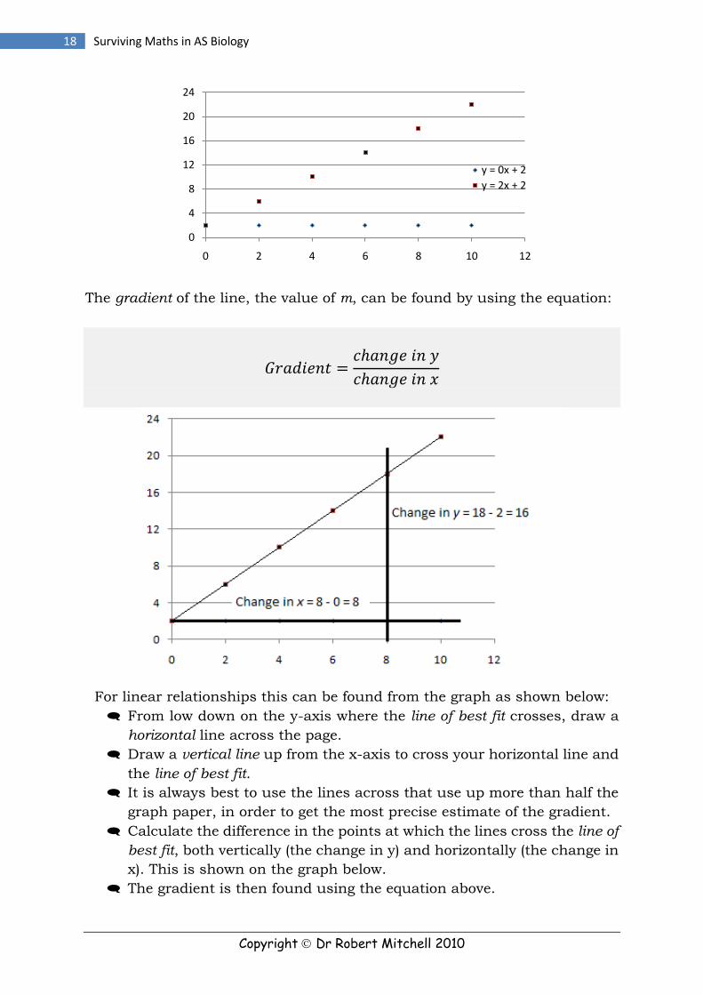
In maths, a linear relationship can be described by the equation y = mx + c
where m is the gradient, the slope of the line and c is the intercept, the point at
which the line crosses the y-axis when x = 0. Consider the table of data below:
When the data are plotted the following
two graphs are obtained. Fitting a straight
line of best fit through the data would
show that when x = 0, y = 2 in both cases,
hence the intercept, c = 2.
x y = 0 x + 2 y = 2x + 2
0 2 2
2 2 6
4 2 10
6 2 14
8 2 18
10 2 22
Copyright Dr Robert Mitchell 2010
18 Surviving Maths in AS Biology
The gradient of the line, the value of m, can be found by using the equation:
For linear relationships this can be found from the graph as shown below:
From low down on the y-axis where the line of best fit crosses, draw a
horizontal line across the page.
Draw a vertical line up from the x-axis to cross your horizontal line and
the line of best fit.
It is always best to use the lines across that use up more than half the
graph paper, in order to get the most precise estimate of the gradient.
Calculate the difference in the points at which the lines cross the line of
best fit, both vertically (the change in y) and horizontally (the change in
x). This is shown on the graph below.
The gradient is then found using the equation above.
0
4
8
12
16
20
24
0 2 4 6 8 10 12
y = 0x + 2
y = 2x + 2

Copyright Dr Robert Mitchell 2010
19 Dr Robert Mitchell
In enzyme reactions, the rate of reaction can be determined experimentally
using this method. When a graph of, for example, mass of product formed is
plotted against time, the gradient of the relationship at any given time is the
reaction rate (expressed in g per second, or g sec-1 in this case).
Notice that at first there is a straight line relationship between mass and time,
so the mass of product formed α (is proportional to) time. As the reaction
proceeds towards completion the graph starts to tail off and become flat.
If the rate of reaction is needed at a given point on this shoulder region, it can
be found by drawing a tangent to the curve and determining its gradient. A
tangent is a straight line or plane that touches a curve or curved surface at a
point but does not intersect it at that point. Calculation of the gradient of the
tangent by using the method outlined above will give the rate of reaction.

Copyright Dr Robert Mitchell 2010
20 Surviving Maths in AS Biology
Frequency tables, pie charts, bar charts and histograms
A frequency table, or tally chart is a means of collecting and organising data
into discrete groups. The data is then often presented as a bar chart or
histogram. Tally charts for sampling biological data usually have two or more
columns, the first of which is for recording the independent variable. If the
independent variable can be numbered (like a weight, height etc) it is
quantitative), if cannot be numbered it is said to be qualitative (like brown
eyes, blue eyes etc).
Categoric data If we were to make a frequency table for animals in a farmer’s field we might
list the different animals in the first column and tally the number (or
frequency) of that animal in the second column. Because the animals fall into
different categories that do not overlap, the data is said to be categoric and
discontinuous. As they aren’t numbers, the data is said to be qualitative.
Animal Frequency Cow 25 Pig 15
Chicken 48 Horse 4
Escapee from prison 2
Such data can be presented on a pie or bar chart. The pie chart represents the
total number of animals as 100%, and is the entire 3600 of the circle. Each
variable is then attributed a slice of the pie whose size is proportional to the
frequency, so the more it is then the bigger the slice. In the example below, 48
out of 94 animals are chickens and so their slice of the pie is just over a half at
51%, or 183.80 and so on for the rest of the animals.
The same data is presented below, but as an unranked bar chart. This time,
the area of their rectangular bar is proportional to the number of animals in
each category.
Cow, 25
Pig, 15Chicken, 48
Horse, 4 Escapee from prison, 2

Copyright Dr Robert Mitchell 2010
21 Dr Robert Mitchell
These kinds of chart are useful for presenting data sampled for discontinuous
variables, but sometimes the data is continuous. In such cases a histogram
is a better option.
Continuous data For variables such as height or weight that show a quantifiable change (a
change you can put a number to) the frequency table can be used to produce
a histogram. Consider the following table showing a distribution of the number
of male students and their heights in a class of AS biology students.
Height Frequency 1.5 - 1.599 2 1.6 - 1.699 7
1.7 - 1.799 18 1.8 - 1.899 4 1.9 - 1.999 1
The independent variable now reflects a change in the heights of the students
from 1.5 meters up to 2 meters and the number of students falling to specified
height groups are tallied and counted. The “bar chart” formed is now termed a
histogram and the data shows the distribution of heights in the student’s
class.
This type of bell-shaped curve is called a normal distribution curve and forms
the basis of some slightly more complex statistical testing which you will
tackle later in the A2.
25
15
48
42
0
5
10
15
20
25
30
35
40
45
50
Cow Pig Chicken Horse Escapee from prison
Frequency

Copyright Dr Robert Mitchell 2010
22 Surviving Maths in AS Biology
If you were to imagine and visualise this data, you would see that “most”
students are of average height with one very tall and two very short class
members. It is this ability to visualise a distribution in different ways which
makes this kind of data presentation a powerful tool in biology.
Scatter diagrams
Scatter diagrams allow a quick and easy means to visualise a relationship
between two sets of numerical data that are paired in some way. They follow a
similar principle to the line graph, except a line or curve does not connect
each successive point; rather the eye is drawn towards the overall trend being
shown.
Consider the following pairs of data which show the relationship between the
number of hours a group of seven students revised for an exam and the
percentage marks they received:
Time spent revising % in exams
0 4
50 87
46 94
11 12
34 75
28 73
39 65
As the hypothesis of the study was to show that the more hours revising
would get a better grade, then the time spent revising was considered to be the
0
2
4
6
8
10
12
14
16
18
20
1.5 - 1.599 1.6 - 1.699 1.7 - 1.799 1.8 - 1.899 1.9 - 1.999
Fre
qu
en
cy
Height (meters)

Copyright Dr Robert Mitchell 2010
23 Dr Robert Mitchell
independent variable. The data are then arranged on a scatter diagram as a
series of x , y (independent , dependent) pairs of data.
A line of best fit can be calculated and placed through the data to further
analyse the relationship between the two variables. If the line goes up, there is
a positive correlation (so the more hours spent revising, the better the result).
If the line goes down then there is a negative or inverse correlation between
the variables.
The gradient of the line, m and the intercept, c can be used to predict what
grade a student might expect for a given number of hours spent revising.
Using the equation y = mx + c in the above example might suggest a student
who worked for 20 hours might expect a (1.86 x 20) + 3.3 = 40.5% in the
exams. But because of the scatter around this line there is a degree of
uncertainty around this estimate.
The more data points there are then the more reliable is the interpretation of
the relationship. In this case there are way too few points to draw a valid
conclusion, but the general pattern is clear.
The investigators would aim to collect more data to see if the relationship held
true in many more situations. The data could also be made more reliable by
filling in the missing data around the 15 to 25 hour mark. Later on you will
learn that this type of association between two variables can be tested to
determine its statistical significance.
y = 1.8599x + 3.3069R² = 0.9028
0
20
40
60
80
100
0 10 20 30 40 50 60
% in exam
Hours spent revising

Copyright Dr Robert Mitchell 2010
24 Surviving Maths in AS Biology
Algebra
Symbols
You are required to know the meaning and context of the following symbols.
A translation is included to show how the mathematics can be interpreted.
These symbols may appear in algebraic expressions or be used in text or
summaries in chemistry. Some examples are given below.
Symbol Translation Example of context
= Is equal to The mass of a shrew = 25 g
< Is less (or lower than) than The mass of a horse < cow
<< Is much less than The mass of a shrew << elephant
> Is greater than Temperature effects > mass effects
>> Is much greater than Chance of catching flu >> developing cancer
α Is proportional to The rate of reaction α concentration
~ Is approximately equal to Biodiversity index of field 1 ~ of field 2
Σ Sum of Total eggs = Σ eggs laid by each hen
% Percent (or out of 100) On average 30% of the day is spent asleep
Rearranging equations
Incorrect equation rearrangements, or changing the subject of an equation as
it is known, accounts for a large percentage of mathematical errors in biology
exams. It’s a skill that many science teachers expect their students to have
already and so they do not show them simple ways of doing it.
There are several rearrangement methods, all of which result in the same
rearrangements if done properly. Two have been included here for you to
choose from. I suggest you practice both and use the one that gives to the
correct answer most of the time.
For Equations involving multiplication and division:
Method 1: Rearrangement In biology the rearrangement of equations such as

Copyright Dr Robert Mitchell 2010
25 Dr Robert Mitchell
are common expectations in exams. You can rearrange these types quickly by
applying the following steps.
For example; to make image size the subject of the equation:
(i) Focus on the subject, the variable you want to find, e.g. image size.
(ii) Whatever another variable is doing to the subject, then do the
opposite to it (divide if it’s multiplying, multiply if it’s dividing), on
both sides of the equation. This means:
(iii) As anything divided by itself = 1, then the above cancels down to:
actual size x magnification = image size
For example; to make actual size the subject of the equation:
(i) If the variable you want to make the subject of the equation is
currently underneath another one, then first of all multiply both
sides by it. This means:
(ii) Cancel this down to get a linear equation:
actual size x magnification = image size

Copyright Dr Robert Mitchell 2010
26 Surviving Maths in AS Biology
(iii) Repeat step (ii) but this time divide both sides by magnification, so:
(iv) Cancelling this down gives the rearranged equation:
Method 2: Linearised method This method is simpler, but it requires you to learn the linearised versions of
the equations first. All you do is learn a linear version and then just put
everything except the subject under the other side of the equation. It’s that
simple! Using the above example, a linear version of the equation would be:
Image size = actual size x magnification
Common linearised equations you will need for AS biology include:
Image size = actual size x magnification
Volume = length x breadth x height
distance = rate x time
Number of bases on DNA = number of amino acids x 3
Cardiac output = stroke volume x heart rate
Pulmonary ventilation = breathing rate x tidal volume
For equations involving addition and subtraction:
The principles involved in rearranging equations with addition or subtraction
is the same as for multiplication in Method 1 above. If the variable you want to
make the subject is positive then do the opposite function (addition or
subtraction) for all other variables, on both sides. For example, to make Ѱs the
subject from the equation Ѱcell = Ѱs + Ѱp:

Copyright Dr Robert Mitchell 2010
27 Dr Robert Mitchell
(i) Ѱcell – Ѱp = Ѱs + Ѱp – Ѱp
(ii) Which simplifies to Ѱcell – Ѱp = Ѱs
(iii) Repeat the process with any other variables present
If the variable you want to make the subject is negative then start by adding
that variable to both sides and then repeating the process outlined above. For
example, to make Ѱp the subject from the equation Ѱs = Ѱcell – Ѱp :
(i) Ѱs + Ѱp = Ѱcell – Ѱp + Ѱp
(ii) Which simplifies to Ѱs + Ѱp = Ѱcell
(iii) Ѱs – Ѱs + Ѱp = Ѱcell – Ѱs
(iv) Hence, Ѱp = Ѱcell – Ѱs
(v) Repeat the process with any other variables present
You are most likely to meet these rearrangements under the osmosis section
of your specification.
Ѱcell = Ѱs + Ѱp
Conversion of Units
SI Units A physical unit gives a sense of scale to a value and allows comparison of
different numbers. As long as, e.g., I know the gram is smaller than a
kilogram, then I know that 20 g of glucose represents a much lower mass than
20 kg. This may be an obvious point but it never ceases to amaze me how
many students completely disregard units and their inter-conversions.
As a general rule of thumb, if the examiners do not ask for a unit then it is best
not to stipulate one. This is because in mark schemes a correct unit is often
seen as neutral whereas an incorrect one can be penalised. This said, many
calculations in biology do require you to interconvert between units and do
clearly specify that you should include a suitable unit in your answer.
As there are so many different units of physical parameters such as
temperature, mass, amount, length, volume, pressure etc., the scientific
community uses an International Standard ( SI ) unit. Smaller or larger
subunits extend out from this, usually in factors of 1000. On the table below,
the units in bold type are the commonest ones for that parameter that you will
use at AS level.

Copyright Dr Robert Mitchell 2010
28 Surviving Maths in AS Biology
1x10⁻⁶ 1x10⁻³ SI unit 1x10³
1x10⁶
Milligram (mg) gram (g) Kilogram (kg) Tonne
Micromole (μmol)
Millimole (mmol)
Mole (mol)
Centimetre cubed (cm3)
Decimetre cubed (dm3)
Meters cubed (m3)
Pascals (Pa) Kilopascals (kPa)
Megapascals (MPa)
If you are converting units from left right, then multiply by the number by
1x10⁻³ (which is the same thing as saying divide by 1000) for each box
covered. So, e.g., 20 mg = 20x10-3 g = 20x10-6 kg etc.
If you are converting units from right left, then multiply by 1x10³ (or times
by 1000) for each box covered. So e.g., 3 tonnes = 3000 kg = 3,000,000 g.
For temperature, the SI unit is the Kelvin, K. The Celsius scale is 2730 lower
than this so:
To convert Celsius to Kelvin, add 273 to the 0C; 250C is 298 K
To convert Kelvin to Celsius, subtract 273 from the K; 0K = -2730C.
Absolutes and concentrations It is important to distinguish between absolutes and concentrations. An
absolute is a physical amount of material, be it 10 g of glucose or 25 dm3 of
carbon dioxide. On the other hand, a concentration represents a certain
amount of a substance in a stated volume. The molar concentration is
expressed in mol dm-3, the same as saying moles per decimetre cubed, or
molarity, M. So a 1 mol dm-3 solution of glucose contains one mole of glucose
dissolved in every decimetre cubed of solution.
In many of the questions you will face, especially those in practicals, you will
have to apply the process of proportions to convert a concentration to an
absolute or vice versa. For example, if there is 1 mole of glucose per decimetre
cubed (1000 cm3) then there is 0.5 mol in 500 cm3 or 0.1 mol in 100 cm3.

Copyright Dr Robert Mitchell 2010
29 Dr Robert Mitchell
Geometry
Two dimensional objects
The formulas for calculating the areas and volumes of common shapes are
shown here to get you familiar with them. You will not be expected to recall
them, but you will be expected to be able to use them.
The area of a square (or rectangle) is found by multiplying its length by its
height and its unit will be mm2, cm2 or m2 depending on the unit of
measurement used:
The circumference (the distance around) of a circle is found by multiplying π
by its diameter (the distance across the centre) and its unit will be mm, cm or
m depending on the unit of measurement used.
The area of a circle is found by multiplying π by its radius (the distance from
the centre of the circle to its edge, or half the diameter) squared and its unit will
be mm2, cm2 or m2 depending on the unit of measurement used:
Three dimensional objects
Most objects in biology are considered to be three dimensional. Even a leaf has
a finite thickness and is not flat. You will learn during your studies that the
surface area of a cell or organism is an important factor that determines its
ability to exchange gases or water. Being able to calculate surface areas

Copyright Dr Robert Mitchell 2010
30 Surviving Maths in AS Biology
and/or volumes of three dimensional objects such as cubes and cylinders can
help to provide models to understand adaptations that some organisms have
to assist their gas exchange processes.
Volume and surface area of a cube A cube is essentially a three dimensional square and as such it
occupies a certain volume of space. This volume (in mm3, cm3,
m3) is found by multiplying its length by its breadth and height.
The cube is composed of six faces, each of which is a square that has an area
that can be found by multiplying its length by its height. It follows then that
the total surface area of the cube is the sum of the areas of each face.
Volume and surface area of a cylinder A cylinder is essentially a circle that has thickness and so it
occupies a volume of space. This volume (in mm3, cm3, m3) is
found by multiplying the area of its circular end by its height.
The cylinder is composed of two circular ends, each of which is a circle that
has an area that can be found by multiplying π by its radius2. The central bar
of the cylinder can be thought of as a rectangle whose length is the height of
the cylinder and whose height is the circumference of the circular end. It
follows then that the total surface area of the cylinder is the sum of the areas
of each face and can be given by the following gobbledegook:

Copyright Dr Robert Mitchell 2010
31 Dr Robert Mitchell
Surface area to volume ratio While the volume and surface area of an organism are important, it is the ratio
of the surface area to the volume (SA:VOL) that is the key to understanding
biological adaptations for gas exchange.
As an organism gets bigger, its volume increases as does its surface area. That
makes complete sense, but what disturbs many students is the fact that the
SA:VOL gets smaller as the organisms gets bigger. This is best shown
mathematically. Consider cubes A and B below.
Cube A has a surface area of
6 cm2 (six faces each having a
1 cm2 area). Its volume is 1
cm3 so its SA:VOL = 6 ÷ 1 = 6.
Cube B has a surface area of
24 cm2 (six faces each having
a 4 cm2 area). Its volume is 8
cm3 so its SA:VOL = 24 ÷ 8 =
3.
The tendency for SA:VOL ratio to decrease as size increases is shown below for
other cubes. This trend is mirrored in other shapes as well but the cube is a
simple model to understand and apply.
0
1
2
3
4
5
6
1 2 3 4 5 6 7 8 9 10
S
A
:
V
O
L
Edge length of a cube (cm)

Copyright Dr Robert Mitchell 2010
32 Surviving Maths in AS Biology
How science works
In the dreaded How Science Works aspect to the specification, you will need to
be familiar with many aspects of studies and study design. The diagram above
tries to separate out these different aspects while at the same time suggesting
how they are all interconnected and exert an impact on one other. For
example, a study that is poorly designed would yield low quality data with
many errors that would confound the analysis and impair the statistical
significance of the result and ultimately lead to an invalid conclusion.
A discussion of these aspects in relation to the mathematics of data handling
is included here to help you familiarise yourself with the ways in which these
aspects impact on the maths questions you will face. A glossary of How
Science Works terms is included at the back of this book to help you keep on
top of the different terms.
How science works
Experimental design
Types of data
Types of variable
ErrorsData quality
Data analysis
Statistical analysis

Copyright Dr Robert Mitchell 2010
33 Dr Robert Mitchell
Types of data
Data are measurements taken in an experiment or study. There are
essentially two types; quantitative (numerical) or qualitative (words).
Quantitative data can be continuous (take any value in a range, e.g. height) or
discrete (discontinuous, e.g. the number of bands on a snake or spots on a
ladybird) whereas qualitative data can be ranked (ordered, e.g. small, medium
or large) or unranked (categoric, e.g. spotted, striped, plain).
The best ways to plot or present the data depends to some degree on the type.
Categoric data suits pie or bar charts best whereas continuous data suits
histograms. Other suitable examples are included further in this book.
Types of variable
Dependent and independent variables In a study, the independent variable (plotted on the x-axis) is changed under
controlled conditions. Measurements are then taken to see how the dependent
variable (plotted on y-axis) is affected by that change. So for example, we may
want to see how the rate of oxygen production from liver is affected by
increasing the concentration of hydrogen peroxide. In this case the
independent variable is the concentration of hydrogen peroxide (x-axis) and
the volume of oxygen measured is the dependent variable (y-axis) as the
Data
Quanitative
numberscontinous / discrete
Qualitative
wordsordered / categoric

Copyright Dr Robert Mitchell 2010
34 Surviving Maths in AS Biology
volume of oxygen formed ultimately depends on the hydrogen peroxide
concentration.
Confounding and control variables Confounding variables are variables that also affect the dependent variable
(e.g. temperature or enzyme concentration in the example above). If a test is to
be declared fair then all the confounding variables must be kept constant and
controlled, e.g. a fixed temperature or amount of liver. If it is not possible to
control the variable, for example the amount of water in soil during a field test,
then they should be monitored closely to assist the analysis and
interpretation of the data. A control variable in a study is a confounding
variable that is kept constant.
Data quality
The quality of the data generated will impact severely on the analysis and
interpretation of the results. Included below is a list of terms that you will
come across time and again. Each term must be internalised and used in its
correct context as these terms are not interchangeable.
True value The real value of a measurement, if it could be recorded with no errors.
Accurate data A measurement that is as close to the true value as the precision allows.
0
2
4
6
8
10
12
14
16
18
20
0 2 4 6 8 10 12
De
pe
nd
en
tva
riab
le
Independent variable

Copyright Dr Robert Mitchell 2010
35 Dr Robert Mitchell
Precise data Measurements that give similar values if repeated and so have a narrow
range. Data that are generated using sensitive equipment with a suitable scale
will generate more precise values (e.g. a thermocouple capable of detecting
0.050C intervals is more precise than a thermometer that can detect 10C
differences in temperature).
Reliable Findings that can be repeated are said to be reliable. Consider a bus which
arrives at 8:01am each day to take you to college would be a reliable service.
One which came randomly between 7:45am and 8:25am would be unreliable
as it did not repeat consistently.
Valid data This is the best quality data as it is both precise and reliable and obtained by
unbiased means in a controlled experiment. In this regard it can be assumed
to be accurate.
Errors
Errors are intrinsic to any study in the real world. They cause the value of the
measurement to vary away from the true or accurate value. There are a
number of different types:
Random These are errors that creep into a study due to inaccuracies, mistakes or poor
techniques. The impact of random errors on the overall results can be
lessened by talking many repeats.
Systematic These are errors which take place in one direction. For example, if a balance
was not calibrated correctly to 10 g and was 1 g too high, then a 10 g weight
would read 11 g and a 20 g weight would read 21 g etc. Systematic errors are
intrinsic to the system and cannot be improved by repetition.
Zero A zero error is a kind of systematic error that results when an instrument, e.g.
a balance does not return to zero after the measurement.

Copyright Dr Robert Mitchell 2010
36 Surviving Maths in AS Biology
Bias Bias occurs when the operator chooses a certain type of result and ignores
others. If, for example the operator had pre-decided that a certain area of
ground had more plants than another, he might sample those parts that had
the greatest density of plants by site as if to prove the point. Bias can be
removed by random sampling which will be discussed in the next section.
Anomaly (outlier) During most investigations some data is generated that might be considered
anomalous, or outlying. Due to biological variation it is often very difficult to
identify whether an anomalous data point is due to an error or a consequence
of variation. Large numbers of repeat measurements can help resolve this
satisfactorily.
Sampling
Biological data has to be collected, or sampled in some way. The method by
which the data is collected has a huge impact on the quality of the results,
their reliability, precision, accuracy etc. This in turn will impact on the validity
of any conclusion that can be drawn.
In a real life situation it is impossible to count every organism or collect every
specimen of a species under investigation. You couldn’t for example count
every daisy in a field, even if you wanted to estimate their density. In such
cases a sample of the population is taken and this is taken in such a way to
ensure that the sample is representative of the population as a whole.
Let’s say we wanted to estimate the population of daisies in a 100 m2 field.
When we look at the field, we notice that there are some areas of the field
where there are lots of daisies and some where there are none. Say we decided
to only take a measurement of daisies in regions where there were lots of
flowers. This would bias the overall result because we have chosen certain
area to suit our aims.
First of all, the only way to avoid bias is to randomly choose which area to take
measurements. The area being sampled could be divided up into a grid and a
number assigned to each grid. A random number generator or table can then
be used to help choose which grid areas are sampled. Secondly, we now face
another problem. How many grids should we sample? If we only sampled one,
and that happened to fall on an area very rich or very poor in daisies, our

Copyright Dr Robert Mitchell 2010
37 Dr Robert Mitchell
results would be inaccurate. But if we sampled too many we would be there all
day and we run the risk of causing damage to the habitat we are studying.
Choosing a compromise of about ten grids allows us to generate data that is
reliable enough to draw a valid conclusion.
By having these repeated measurements, we would then be able to analyse
the data and perform a statistical analysis to help us assess the significance of
the results we have found.
Data analysis
Once the data has been sampled it can be transformed, manipulated and
summarised to help us view it in such as way as to draw conclusions. Often
the first step is to calculate an average of the data (mean, mode or median)
and to look at the range, or standard deviation in the data.
Means, modes and medians are all types of average, but each one can give a
different value. One type of average may be more appropriate than another in
different contexts. In AS biology the most common type of average is the
mean, but you must also be aware of how the others are calculated.
Consider the list of data; 1, 2, 2, 3, 4, 7, 9. Using this simple data set shows
the differences in the values that can be obtained. The arithmetic mean would
be 4, the median is 3 and the mode is 2. How each is calculated is shown
below.
Arithmetic Mean A mean is one of three kinds of mathematical average (mode and median are
others). The mean is found using the equation:
Most people use the principle, “add them all up and divide by how many there
are.” For example to find the average of 1, 2, 2, 3, 4, 7, and 9 the equation is
used:

Copyright Dr Robert Mitchell 2010
38 Surviving Maths in AS Biology
One common error is to fail to check that the average value calculated lies within the range
of the numbers being averaged. So in the example above 4 does lie between 1 and 9.
Mode The mode is the most frequent number in a set of data, or the most likely value
to be sampled. So in the set 1, 2, 2, 3, 4, 7, 9, the number 2 appears more
times than the others and so that is the mode of this data set.
Median The median is the value that separates the higher half of the sample from the
lower half. This is found by placing the data in a rank of increasing numbers;
1, 2, 2, 3, 4, 7, 9. As there is an odd number of data points, the number at the
central position is the median. In this case it is the number 3, at the fourth
position as there are three numbers smaller, and three numbers higher than
it.
For even data sets, there are two central numbers and the median is the
average of those two numbers. For example, if the data set was 1, 2, 2, 2, 3, 4,
7, 9 then the central two numbers are 2 and 3 and so the median would be the
average of 2 and 3, which is 2.5.
Determine the mean, mode and median of the following data set;
10, 15, 18, 7, 7, 14, 5.
Mode = most frequent number = 7
Median
(i) rank the data; 5, 7 , 7, 10, 14, 15, 18 (ii) = select the central value = 10 (three lower, and three higher values)

Copyright Dr Robert Mitchell 2010
39 Dr Robert Mitchell
Range The range of the data is essentially the difference between the top and bottom
values of the ranked data. In the data set from the section above (1, 2, 2, 3, 4,
7, 9) the data ranges from 1 to 9. So if we were to consider the range of heights
of male students in an AS biology class, they may range from 1.5 to 1.99
meters; a span of 0.49 meters.
Standard deviation The range may give an accurate indication of the top and bottom values in a
set of data, but it does not reflect the spread of the data and the fact that most
of these students might be between 1.6 and 1.68 with the rest being outliers.
The standard deviation is used as a better indication of the spread around the
mean. It is a statistical concept that you’ll learn how to calculate in A2 as part
of the ISA/EMPA aspect of the specification. At this stage you do not need to
know how to calculate it, but need to recognise that the bigger the standard
deviation, the more spread the data.
In a normal distribution, the bell shaped curve, one standard deviation
around the mean encompasses 68.2% of the data points around the mean
value. Two standard deviations encompass 95.4% of the data points.
Put simply, about two thirds of the members of the class would have a height
that lay within one standard deviation from the mean height. Such data is
often expressed as mean ± one standard deviation. We might say the average
height of male students in the class is 1.73 ± 0.2 meters. In this case we

Copyright Dr Robert Mitchell 2010
40 Surviving Maths in AS Biology
would know that 68%, about two thirds of the guys had a height between 1.53
(1.73 - 0.2) and 1.93 (1.73 + 0.2) meters.
Statistical analysis
When a study is designed, it is attempting to test a hypothesis and answer a
particular question, or problem. A hypothesis can be defined as a possible
explanation of a problem that can be tested experimentally. Generally at
A-level there are three main types question you will attempt to answer using
statistical tests (i) whether there is a difference between measurements of
different samples using a t-test, standard error or 95% confidence
intervals, (ii) quantify a relationship between two variables using a rank
correlation, or (iii) finding the number of individuals in certain categories and
determine if their distributions are different using a chi-squared test.
Thankfully you’ll not be expected to remember the formulae for the
calculation but you will be expected to plug in the numbers for data in
practical or ISA or EMPA questions.
Central to the idea of testing a hypothesis, is a null hypothesis. This is
worded in terms of there being no difference or association between the two
variables being compared (it’s the negative version of a hypothesis). So if I
wanted to test the hypothesis that the more hours I spend revising would get
me a better exam result, I would need to test this against the null hypothesis
that it would not.
Probability
The statistical tests generate test statistic which can then be used to help
determine whether the event occurred by chance. The certainty of this is
affected by the number of estimations or counts or measurements that were
taken. It ought to be obvious that the more measurements we take then the
more certain we should be of a certain result. These estimations are referred
to statistically as the degrees of freedom. The greater the number of degrees
of freedom, then the more certain we can be that an event was significant, and
not due to a chance happening.
The test statistic and the degrees of freedom combine to determine the
probability. Probability is the likelihood of an event occurring. It is different

Copyright Dr Robert Mitchell 2010
41 Dr Robert Mitchell
from chance because it can be expressed mathematically. When a statistical
test is performed on data it generates a p-value. This is essentially an
estimate of whether a finding is due to chance.
The probability of an absolutely impossible event happening is zero, 0. The
probability an absolutely certain event happening is one, 1. Statistical tests
generate values within this range. It is up to us as the investigators to decide
an acceptable level of probability that an event is not due to chance.
A p-value of 0.05 of less is generally considered by scientists to be significant
as it means there is less than a 5% probability that the result was due to
chance. In other words, if we were to do the investigation 100 times, 95 of
them would generate data to support the hypothesis where five would support
the null hypothesis, So a p<0.05 would mean that the null hypothesis is
rejected and the result is deemed a statistically significant one.

Copyright Dr Robert Mitchell 2010
42 Surviving Maths in AS Biology
End of Section 1 Test
Fractions, decimals, ratios and percentages
1. Express the following fractions as (i) percentages, (ii) decimals and (iii)
standard form. Give all you answers to three significant figures:
a.
(i) % (ii) (iii)
b.
(i) % (ii) (iii)
c.
(i) % (ii) (iii)
2. In a recent college biology test it was shown that 18 of out every 57
students gained a grade B or above.
a. Express this information as (i) a percentage, (ii) a decimal and (iii)
in standard form. Give all your answers to three significant
figures.
(i) % (ii) (iii)
b. Another teacher is setting the same test. How many students
would he expect to achieve a grade B or above from a class of 36?
____________________
c. Using the same test a third teacher found that four students
gained grade B or above. How many students were in her class?
__________________
Score ______ / 14 [ __________ %]
Copyright Dr Robert Mitchell 2010
43 Dr Robert Mitchell
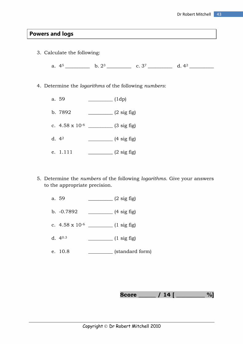
Powers and logs
3. Calculate the following:
a. 45 __________ b. 23 __________ c. 37 __________ d. 42 __________
4. Determine the logarithms of the following numbers:
a. 59 __________ (1dp)
b. 7892 __________ (2 sig fig)
c. 4.58 x 10⁻⁶ __________ (3 sig fig)
d. 42 __________ (4 sig fig)
e. 1.111 __________ (2 sig fig)
5. Determine the numbers of the following logarithms. Give your answers
to the appropriate precision.
a. 59 __________ (2 sig fig)
b. -0.7892 __________ (4 sig fig)
c. 4.58 x 10⁻⁶ __________ (1 sig fig)
d. 40.3 __________ (1 sig fig)
e. 10.8 __________ (standard form)
Score ______ / 14 [ __________ %]

Copyright Dr Robert Mitchell 2010
44 Surviving Maths in AS Biology
Rearranging equations
6. By rearranging the equation A x B x C = D x E x F , make each of the
following the subject of the equation:
(i) A =
(ii) C =
(iii) D =
(iv) E =
7. Rearrange the following equation
(i) B =
(ii) C =
(iii) D =
(iv) E =
8. By rearranging the equation A +B - C = D + E - F , make each of the
following the subject of the equation:
(i) A =
(ii) B =
(iii) C =
(iv) E =
(v) F =

Copyright Dr Robert Mitchell 2010
45 Dr Robert Mitchell
9. Rearrange the following equation
(i) B =
(ii) C =
(iii) 1000 =
Score ______ / 16 [ __________ %]
Unit conversions
10. Express the following masses as the specified units:
a. 10 g = __________ kg c. 145 kg = __________ g
b. 802 mg = __________ kg d. 14 mg = __________ g
11. Express the following volumes as the units specified n the
questions:
a. 100 cm3 = _________ dm3 c. 24 dm3 = _________ cm3
b. 802 m3 = _________ cm3 d. 0.01 dm3 = _________ m3
Score ______ / 8 [ __________ %]

Copyright Dr Robert Mitchell 2010
46 Surviving Maths in AS Biology
Gradient, intercept and rate
12. Plot a graph of the following data and use it to deduce the missing
volumes, and calculate the gradient and intercept of the line [6 marks].
Time (seconds) Volume of CO2 released (cm3)
5 18
10 33
15 48
20 ?
25 ?
30 93
Score ______ / 8 [ __________ %]
Grand total of ___________ / 60 = ___________ %
0
20
40
60
80
100
0 5 10 15 20 25 30 35

Copyright Dr Robert Mitchell 2010
47 Dr Robert Mitchell
End of Section 1 Test Answers
Fractions, decimals, ratios and percentages
1. Express the following fractions as (i) percentages, (ii) decimals and (iii)
standard form. Give all you answers to three significant figures:
a.
(i) 6.17 % (ii) 0.0617 (iii) 6.17x10⁻²
b.
(i) 21.1 % (ii) 0.211 (iii) 2.11x10⁻¹
c.
(i) 0.800 % (ii) 0.008 (iii) 8.00x10⁻³
2. In a recent college biology test it was shown that 18 of out every 57
students gained a grade B or above.
a. Express this information as (i) a percentage, (ii) a decimal and (iii)
in standard form. Give all your answers to three significant
figures.
(i) 31.6 % (ii) 0.316 (iii) 3.16x10⁻¹
b. Another teacher is setting the same test. How many students
would he expect to achieve a grade B or above from a class of 36?
11
c. Using the same test a third teacher found that four students
gained grade B or above. How many students were in her class?
13
Score ______ / 14 [ __________ %]
Copyright Dr Robert Mitchell 2010
48 Surviving Maths in AS Biology
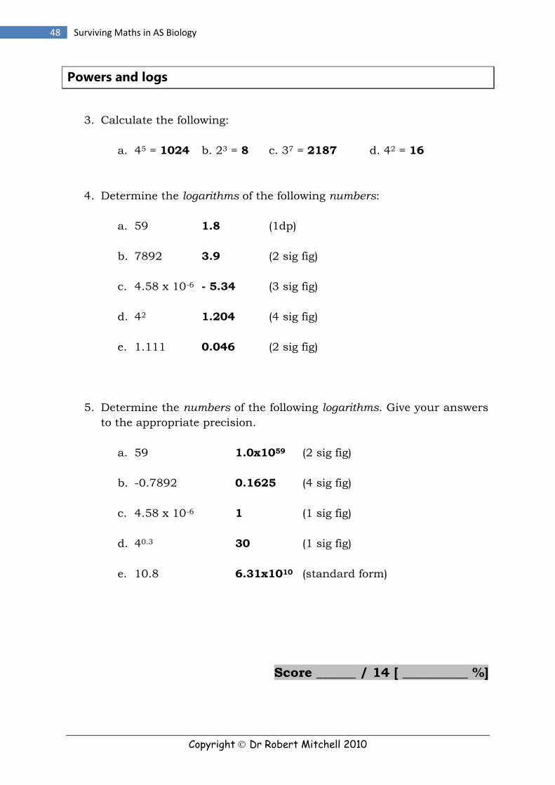
Powers and logs
3. Calculate the following:
a. 45 = 1024 b. 23 = 8 c. 37 = 2187 d. 42 = 16
4. Determine the logarithms of the following numbers:
a. 59 1.8 (1dp)
b. 7892 3.9 (2 sig fig)
c. 4.58 x 10⁻⁶ - 5.34 (3 sig fig)
d. 42 1.204 (4 sig fig)
e. 1.111 0.046 (2 sig fig)
5. Determine the numbers of the following logarithms. Give your answers
to the appropriate precision.
a. 59 1.0x1059 (2 sig fig)
b. -0.7892 0.1625 (4 sig fig)
c. 4.58 x 10⁻⁶ 1 (1 sig fig)
d. 40.3 30 (1 sig fig)
e. 10.8 6.31x10¹⁰ (standard form)
Score ______ / 14 [ __________ %]

Copyright Dr Robert Mitchell 2010
49 Dr Robert Mitchell
Rearranging equations
6. By rearranging the equation A x B x C = D x E x F , make each of the
following the subject of the equation:
(i) A =
(ii) C =
(iii) D =
(iv) E =
7. Rearrange the following equation
(i) B =
(ii) C =
(iii) D =
(iv) E =
8. By rearranging the equation A +B - C = D + E - F , make each of the
following the subject of the equation:
(i) A = D + E – F – B + C
(ii) B = D + E – F – A + C
(iii) C = A + B – D – E + F
(iv) E = A + B – C – D + F
(v) F = D + E – A – B + C

Copyright Dr Robert Mitchell 2010
50 Surviving Maths in AS Biology
9. Rearrange the following equation
(i) B = ( 1000 A ) - C
(ii) C = ( 1000 A ) - B
(iii)
Score ______ / 16 [ __________ %]
Unit conversions
10. Express the following masses as the specified units:
a. 10 g = 0.01 kg c. 145 kg = 145 000 g
b. 802 mg = 8.02x10⁻⁴ kg d. 14 mg = 0.014 g
11. Express the following volumes as the units specified n the
questions:
a. 100 cm3 = 0.1 dm3 c. 24 dm3 = 24 000 cm3
b. 802 m3 = 8.02x106 cm3 d. 0.01 dm3 = 1x10⁻⁵ m3
Score ______ / 8 [ __________ %]

Copyright Dr Robert Mitchell 2010
51 Dr Robert Mitchell
Gradient, intercept and rate
12. Plot a graph of the following data and use it to deduce the missing
volumes, and calculate the gradient and intercept of the line [6 marks].
Time (seconds) Volume of CO2 released (cm3)
5 12
10 22
15 32
20 42 [1 mark] 25 52 [1mark] 30 62
[1 mark] correctly labelled x-axis [1 mark] correctly labelled y=axis
[1 mark] correctly plotted points [1 mark] line placed through data
[1 mark] gradient = 2 [1 mark] intercept = 2
Score ______ / 8 [ __________ %]
Grand total of ___________ / 60 = ___________ %
Copyright Dr Robert Mitchell 2010
52 Surviving Maths in AS Biology
Section 2: Calculations in AS
Biology Specifications
Very few concepts in biology strike fear into the hearts of students like data
handling questions. A close second is magnification because of the conversion of
units, and the AS biology specs have both! If the teacher doesn’t put it in the
right way at the start then your confidence in these relatively straight forward
concepts gets dented, and it often doesn’t recover even by A2. This section puts
this right, and shows you just how to go about the calculation content without the
fear...

Copyright Dr Robert Mitchell 2010
53 Dr Robert Mitchell
The art of reading questions
Too many people misread the question and lose marks pointlessly. They
describe when they should have explained; did not use the data when asked
to, or failed to use figures when describing graphs.
While each board publishes their own glossary of terms, it is possible to
combine them into a clear set of instructions you can follow to help you
answer the questions appropriately. The terms below represent the ones that
are most relevant for the mathematical requirement.
Criteria Instruction
Analyse and interpret Identify the essential features of the information or data
provided. There should be reasons behind the features and it’s
likely that some data manipulation would be expected.
Appreciate Show awareness of the significance of the data or underlying
principles but without detailed knowledge.
Brief Short statements of only the main points.
Calculate Work out an answer & show a clear route of derivation to the
answer.
Compare Discuss the similarities and differences between two or more
variables. Outline similarities and differences separately.
Contrast Like compare, but the emphasis will be on differences.
Criticise Highlight any faults, shortcomings or limitations of an experiment.
Describe Simply put; “Say what you see with figures”. Any descriptions
must relate directly to the information provided. It must be
concise and straight-forward. Any trend should be presented in
words or translated mathematically. If numerical data is being
described, there must be specific references to figures. Figures
should normally be manipulated in some way (e.g. percentage
changes etc).
Distinguish Identify any appropriate differences.
Evaluate To judge or determine the significance of the information. States
what’s good and bad about the conclusions.
Graphs Be careful to take notice of any specific instructions given in the
question. Plot in pencil so corrections are possible. Always make
the maximum use of the graph paper for greatest precision. Axes
should be fully labelled and include the units of variables. Always
use rulers or flexi-curves to join points. Never use sketchy lines.
Using the data or information
Numerical answer must be provided using the provided data as a
direct source.

Copyright Dr Robert Mitchell 2010
54 Surviving Maths in AS Biology
Magnification questions
Magnification and actual size
Cells and their organelles are structures that can only be viewed using light or
electron microscopes. These instruments magnify the image many times and
make it visible. The size of the image you see, the actual size of the organelle
and the magnification are all linked by the equation:
In other words, magnification is a ratio of how big something appears
compared to its real size. This equation is deceptively simple but it is fraught
with tricks that tend to cause common errors. One of the biggest of these is
the unit conversions involved. Cell sizes are almost exclusively reported in
microns, µm (1x10⁻⁶ meters), whereas the actual image size can be measured
on the exam paper in mm or cm. To avoid any difficulties whatsoever, follow
these rules exactly:
1. Measure the image size in mm.
2. Multiply the measurement by 1000 to convert it to microns.
3. Rearrange the equation above depending on what the question is
asking for.
There are two types of questions that use this kind of approach; (i) calculation
of magnification from an image, (ii) calculation of actual size from the
magnification.
Worked example 1: The image below is of a nucleus of an epithelial cell viewed by an electron microscope. The actual size of the organelle shown is 2.5µm. Use this information to calculate the magnification of the diagram.
Image diameter = 18 mm X 1000 = 18 000 µm

Copyright Dr Robert Mitchell 2010
55 Dr Robert Mitchell
Worked example 2: The image below is of a mitochondrion in a skin cell viewed by a transmission electron microscope. The magnification of the diagram is x12 000. Use this information to calculate the actual length of the organelle.
Image length = 16 mm X 1000 = 16 000 µm
Actual size using a scale bar
Some questions provide the student with a scale bar and demand a
calculation of the actual size of a cell or organelle. These questions use ratios
to determine the answer, so follow these instructions:
1. Measure the length of the scale bar in mm and multiply the
measurement by 1000 to convert it to microns.
2. Measure the length of the image of the cell or organelle in mm and
multiply the measurement by 1000 to convert it to microns.
3. Find the ratio of cell length : scale bar length by dividing the length of
the structure by the length of the scale bar.
4. Multiply the size shown on the scale bar by that many times to get
the actual size of the structure.
Worked example 3: The diagram below shows the image of a palisade cell of a plant. Using the information provided, calculate (i) the maximum length of the palisade cell, and (ii) given that the length of organelle X is 8 µm, calculate the magnification of the diagram.

Copyright Dr Robert Mitchell 2010
56 Surviving Maths in AS Biology
(i) Length of scale bar = 7.5 mm = 7500 µm Length of image of cell = 52 mm = 52 000 µm
Ratio cell : scale bar = 52000 / 7500 = 6.93 Actual cell length = 6.93 x 5 = 34.7 µm
(ii) Image diameter = 12 mm X 1000 = 12 000 µm
Always do measurements in mm never cm.
Heart, breathing and cycle rates
Like many organs and systems, the heart and lungs follow a pattern of cyclical
changes that repeat after a certain time interval. Each cycle therefore takes a
specific amount of time to complete. The rate (cycles per unit time) can be
found by dividing the time unit by the time of one cycle.
Other cycles follow a similar pattern, the only difficulty that you will face in
the questions is being conscious of the units involved; whether the rate is
cycles per second, minutes or hours.
All these cyclical questions are based around the equation that you will
probably be familiar with from GCSE physics:
distance = speed x time
Almost all the questions will be in the form of graphs. The independent
variable on the x-axis will usually be time in a specified unit. To determine the
length of time it takes for one cycle:

Copyright Dr Robert Mitchell 2010
57 Dr Robert Mitchell
1. Identify a point on two cycles that are at the same point on the cycle.
2. For each point read the value of the x-axis (time).
3. The length of one cycle = higher time – lower time.
4. The cycle rate (per minute) = 60 ÷ length of one cycle
Worked example 4: The diagram below shows the pressure changes in
three chambers of the heart during the cardiac cycle. Use the graph to
calculate (i) the time taken for one heart beat, and (ii) the heart rate of the
of the individual shown. Give a suitable unit.
(i) Common point on both cycles where the aorta crosses the left ventricle;
is 0.9 – 0.14 = 0.76 seconds
(ii) Heart rate = 60 ÷ 0.76 = 79 beats per minute.
Worked example 5: The vole is a small mammal that has a much higher metabolic rate than a human. The diagram over the page shows the pressure changes in the aorta of a vole. Use the graph to calculate the heart rate of the vole. Give a suitable unit in your answer.

Copyright Dr Robert Mitchell 2010
58 Surviving Maths in AS Biology
The common point on all the cycles is at the base of the cycles; 450 – 360 = 90 milliseconds. 90 milliseconds = 90x10-3 seconds. Heart rate = 60 ÷ 90x10-3 = 667 beats per minute.
Osmosis
Osmosis is the net movement of water across a partially permeable membrane
from an area of high water potential (high concentration of water) to an area of
lower water potential (lower concentration of water). It is usually expressed as
a pressure in units of kPa.
When the water potential of the surrounding solution is higher than that
inside the cell, water moves into the cell by osmosis and the cell will swell up.
When the water potential of the surrounding solution is lower than that inside
the cell, water moves out of the cell by osmosis and the cell will shrivel up.
The two common types of question at AS are using the equation Ѱcell = Ѱs + Ѱp
and also those involving the experimental determination of the concentration
at which the water potential of a solution is equal to the water potential of
plant tissues such as potato tuber.

Copyright Dr Robert Mitchell 2010
59 Dr Robert Mitchell
Ѱcell = Ѱs + Ѱp
The water potential of a cell is given by, Ѱcell = Ѱs + Ѱp where Ѱcell is the water
potential of the cell and Ѱs and Ѱp are the solute potential and the pressure
potential respectively. The key to these types of question is being able to
rearrange the equation correctly.
Worked example 6: The table below shows some values of water potential for three adjacent cells in the leaf of a plant. Use your knowedge of the relationship between the water potential of the cell, Ѱcell and solute
potential, Ѱs and pressure potential, Ѱp to fill in the blank values of the table.
Cell Ѱcell (kPa) Ѱs (kPa) Ѱp (kPa)
A – 1400 + 600
B – 400 + 300
C –1000 – 800
Fill in the missing boxes.
Cell Ѱcell (kPa) Ѱs (kPa) Ѱp (kPa)
A – 800 = – 1400 + 600 – 1400 + 600
B – 400 – 700 = – 400 – 300 + 300
C –1000 – 800 – 200 = – 1000 – –800
Experimental determination of water potential
This is an experiment you may even have done at GCSE, you know the one!
Chop up pieces of potato or carrot and leave them for a few hours in different
solutions of a range of solute (sucrose or sodium chloride) concentrations. If
the water potential of the solution is higher than that of the potato, water
moves into the cells by osmosis and the potato increases its length or mass.
Conversely if the water potential of the solution is lower than the potato, water
moves out of the cells by osmosis and the length or mass decreases.
The objective of this experiment is to determine the concentration of solute
which has the same water potential as the potatoes; at this point the water
potentials will be equal and there will be no net movement of water. In other
words the change in mass will be zero. If a ratio of final mass (or length) to

Copyright Dr Robert Mitchell 2010
60 Surviving Maths in AS Biology
initial mass (or length) is used then the ratio when the water potentials are
equal will be 1. It is the data handling aspect of this experiment is what makes
it of particular interest to examiners.
1. Plot a graph of solute concentration (independent variable, x-axis)
against the ratio of final to initial mass or weight (dependent variable,
y-axis).
2. A ratio is used to standardise the data against small differences in
initial mass.
3. Draw a line of best fit through the data.
4. Identify the concentration of solute which gives a ratio of 1 (no net
movement of water).
Worked example 7: A student designed an experiment to investigate the effect of sucrose concentration on the masses of 5 mm cubes of potato tuber cut from a single potato. He rinsed and dried each cube and placed it in a certain sucrose concentration for 4 hours. He then dabbed the cubes on tissue paper to remove excess solution and re-weighed them.
Sucrose (mol dm-3) 0.2 0.3 0.4 0.5 0.6 0.7
Ratio of initial to final length 0.6 0.78 0.95 1.1 1.25 1.4
Plot a graph of the data and use it to determine the concentration of sucrose which has the same water potential as the pieces of potato.
The water potential of the potato is the same as the sucrose concentration when the ratio is 1, = 0.45 mol dm-3.
Look carefully; if you use a ratio (read off at 1) or difference in mass (read off at 0)
0
0.5
1
1.5
0 0.1 0.2 0.3 0.4 0.5 0.6 0.7 0.8
Rat
io I:
F
Sucrose concentration (mol dm-3)

Copyright Dr Robert Mitchell 2010
61 Dr Robert Mitchell
Nucleotide bases in DNA/RNA
Number of bases on DNA and amino acids in proteins
Nucleic acids such as deoxyribonucleic acid, DNA and ribonucleic acid, RNA
carry the genetic code that determines the primary structure of proteins. The
code is a triplet code as three bases on DNA or RNA code for one amino acid
in the peptide chain. It follows that:
number of bases on DNA = number of amino acids x 3
Worked example 8: As part of the human genome project scientists determined the sequence of bases on all human genes. One gene on chromosome 12 was composed of 927 bases on its DNA. What is the maximum number of amino acids in the protein that is coded for by this gene?
Worked example 9: Some proteins have quaternary structure and are made up of two or more tertiary structures combined together. One such protein is made up of two subunits. Subunit A has 8000 amino acids and subunit B has 3300 amino acids. Deduce the number of bases on DNA required to code for the finished protein.
Total number of amino acids in finished protein = 8000 + 3300 = 11300
Number of bases on DNA = 11300 x 3 = 33900 or 33903*
*You will often see in mark schemes that an alternative answer that is three more
bases is allowed. This is because of the stop codon that some teachers cover in AS.
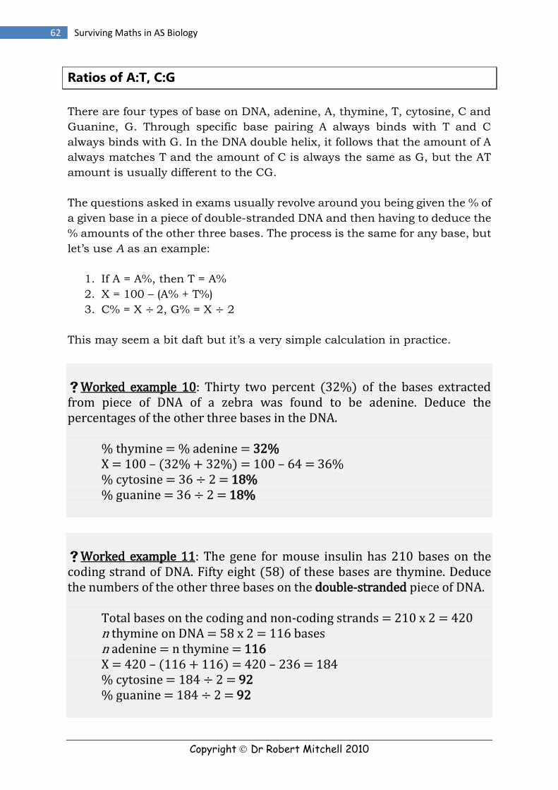
Copyright Dr Robert Mitchell 2010
62 Surviving Maths in AS Biology
Ratios of A:T, C:G
There are four types of base on DNA, adenine, A, thymine, T, cytosine, C and
Guanine, G. Through specific base pairing A always binds with T and C
always binds with G. In the DNA double helix, it follows that the amount of A
always matches T and the amount of C is always the same as G, but the AT
amount is usually different to the CG.
The questions asked in exams usually revolve around you being given the % of
a given base in a piece of double-stranded DNA and then having to deduce the
% amounts of the other three bases. The process is the same for any base, but
let’s use A as an example:
1. If A = A%, then T = A%
2. X = 100 – (A% + T%)
3. C% = X ÷ 2, G% = X ÷ 2
This may seem a bit daft but it’s a very simple calculation in practice.
Worked example 10: Thirty two percent (32%) of the bases extracted from piece of DNA of a zebra was found to be adenine. Deduce the percentages of the other three bases in the DNA. % thymine = % adenine = 32% X = 100 – (32% + 32%) = 100 – 64 = 36% % cytosine = 36 ÷ 2 = 18% % guanine = 36 ÷ 2 = 18%
Worked example 11: The gene for mouse insulin has 210 bases on the coding strand of DNA. Fifty eight (58) of these bases are thymine. Deduce the numbers of the other three bases on the double-stranded piece of DNA.
Total bases on the coding and non-coding strands = 210 x 2 = 420 n thymine on DNA = 58 x 2 = 116 bases
n adenine = n thymine = 116 X = 420 – (116 + 116) = 420 – 236 = 184 % cytosine = 184 ÷ 2 = 92 % guanine = 184 ÷ 2 = 92

Copyright Dr Robert Mitchell 2010
63 Dr Robert Mitchell
Index of diversity
Diversity index is a measure of species diversity in a given area or habitat. It is a better indicator of diversity than a simple number of different species
present as it not only considers the range of species present but also takes into account the abundance of each species. The index of diversity, d is given
by:
and n = total number of organisms of each species
Worked example 12: Calculate the diversity index, d for the two habitats X and Y from the data below.
Species found Numbers found in habitat X Numbers found in habitat Y
A 10 3
B 10 5
C 10 2
D 10 36
E 10 4
Number of species 5 5
No. of individuals 50 50
First calculate n (n-1) for each species in the habitat. Next calculate the sum of, ∑ n(n-1) by adding them all up.
Species Numbers (n) found in X
n(n-1) Numbers (n) found in Y
n(n-1)
A 10 10 x 9 = 90 3 3 x 2 = 6
B 10 10 x 9 = 90 5 5 x 4 = 20
C 10 10 x 9 = 90 2 2 x 1 = 2
D 10 10 x 9 = 90 36 36 x 35 = 1260
E 10 10 x 9 = 90 4 4 x 3 = 12 ∑ n(n-1) 450 ∑ n(n-1) 1300

Copyright Dr Robert Mitchell 2010
64 Surviving Maths in AS Biology
0255075
100
0 10 20 30 40
0255075
100
0 10 20 30 40
0255075
100
0 10 20 30 40
Data handling and interpretation
The data handling component seems to concern many students as it appears
at first sight that they can ask anything. The fundamentals of data handling
are straight forward enough, it just takes a bit of practice and confidence to
apply them. In this section you will find out how to standardise descriptions
and give some relatively standard answers to some seemingly non-standard
questions.
Describing lines
Describing graphs and the changes they show is a fundamental expectation in
the A-level exams that's usually worth between 2 and 4 marks. Since the
introduction of a much more involved How Science Works component, some
boards (Edexcel and AQA for example) seem to put a greater emphasis on the
data handling skill and so there can be more marks available for description.
And they are easy marks in that you are saying what you see with figures, and
as such do not require any prior biological knowledge.
Included below are a variety of different shaped graphs that are of a type often
used in exams. Each one is accompanied by a simple and standardised way of
describing it that would get the marks. Remember that if this was a real exam
you would substitute in time or mass or whatever the axis was instead of
saying x and y.
As x increases from 0 to 40, y increases
proportionally up to 100.
As x increases from 0 to 20, y increases
proportionally. When x > 20 y remains constant at
100.
As x increases from 0 to 40, y increases with a
gradient that gets steeper as x increases.

Copyright Dr Robert Mitchell 2010
65 Dr Robert Mitchell
0255075
100
0 10 20 30 40
0255075
100
0 10 20 30 40
0255075
100
0 10 20 30 40
0255075
100
0 10 20 30 40
0255075
100
0 10 20 30 40
0255075
100
0 10 20 30 40
0255075
100
0 10 20 30 40
As x increases from 0 to 40, y remains constant at
50.
As x increases from 0 to 40, y decreases
proportionally.
As x increases from 0 to 20, y decreases
proportionally. When x > 20 y remains constant at
50.
As x increases from 0 to 40, y decreases with a
gradient that gets less steep as x increases.
As x increases from 0 to 20, y increases
proportionally up to a maximum of 100. As x
continues to increase above 20 y decreases
proportionally to 0.
As x increases from 0 to 20, y decreases
proportionally to a minimum of 0. As x continues to
increase above 20 y increases proportionally to 100.
As x increases up to 40, y increases with a
decreasing gradient up to a maximum of 100.

Copyright Dr Robert Mitchell 2010
66 Surviving Maths in AS Biology
0255075
100
0 10 20 30 40
0255075
100
0 10 20 30 40
Comparing lines
When comparing two graphs the key is to visualise any similarities and
differences. Like with description, using figures here will be of fundamental
importance to scoring the maximum marks.
For both curves A and B as x increases up to 20, y
increases proportionally, with both A and B having
the same gradient. When x > 40, A continues to
increase proportionally whereas B remains constant
at 50.
For both curves, as x increases y increases
proportionally and then it remains constant at the
same value at 75. The gradient of B is lower than the
gradient of A.
There are so many different combinations that could be asked but the
principle is the same, say what is similar and what is different about the two
lines.
Data manipulation
When using experimental data it is often necessary to manipulate the data in
some way to help visualise the trends and make interpretation clearer. In
many data handling questions there are certain themes and calculations
which recur in different contexts. Included below is a list of standard contexts
and guidelines on how to deal with them effectively.
Standardisation of y-axis data
Percentages
Percentages express fractions out of 100. It is a way of making data more
instantly comparable. For example the data were to show a decrease in the
serum cholesterol levels at varying times on a certain drug; the data may be
expressed at a % of the original cholesterol level. It allows a comparison as
these initial values were not identical to start with.

Copyright Dr Robert Mitchell 2010
67 Dr Robert Mitchell
Ratio
Ratios are like percentages in that they allow a comparison of data in cases
where the initial amounts of start materials may have varied. In osmosis
studies it is common to study the change in mass, or length of a piece of
potato or beetroot when exposed to different concentrations of sucrose
solution. A ratio of final length to initial length in an osmosis study gives a
clear indication of whether water had a net movement into or out of cells. The
ratio is used, rather than the absolute changes in mass or length because the
initial masses or lengths varied slightly.
Difference in mass or length
This is a manipulation similar to taking a ratio. It is not as useful as using a
ratio as the amount it changes by may also depend on the initial value.
Expressing data as “something per something”
The data on the y axis can be expressed as x per y or out of y (e.g. number of
cases per 100 000 people, or amount of food per gram of mouse). They will ask
you why the data is expressed per something. The standard 2 mark answer:
[1] It allows a comparison, [1] because ______ differs or changes.
For example; the number of deaths per 100 000 people is proportional to the
amount of saturated fat in the diet of different countries. The data is
expressed per 100 000 people as it allows a comparison because the
number of people in each country is different.
For example; the blood concentration of a drug per kg of body mass is
proportional to the BMI of the patient in a variety of ethnic groups studied.
The data is expressed per kg of body mass as it allows a comparison because
the body masses of the ethnic groups varied.
% increase and decrease
If by changing the independent variable there is an increase in the dependent
then it is common to ask you to calculate this change as a % increase rather
than an absolute change. This can be calculated using the equation.

Copyright Dr Robert Mitchell 2010
68 Surviving Maths in AS Biology
Worked example 13: The data below shows the effect of a male fertility drug on the numbers of sperm produced by men over a 6 month period of treatment. Use the data to calculate (i) the percentage increase in sperm counts between months 1 and 3 and (ii) the % decrease in sperm count between months 5 and 6.
Treatment month Sperm count (millions / cm3)
0 84
1 82
2 86
3 93
4 120
5 176
6 89
A simple way of remembering which way round it is, is to imagine your start
point; So if it is a decrease you are starting big and going little (so you divide
by big) and if it is an increase you are starting little and going big (so you
divide by little).

Copyright Dr Robert Mitchell 2010
69 Dr Robert Mitchell
0255075
100
0 10 20 30 40
0255075
100
0 10 20 30 40
Causation and correlation
All the boards are keen on testing your appreciation of the difference between
causation and correlation. Causation is a change in one variable that results
from (or is caused by) a change in another variable (a change in one causes
the other to change as well). A correlation shows a relationship between two
variables. Evidence of correlation does not automatically imply causation.
The simplest way to distinguish between causation and correlation is to use a
scatter diagram:
Causation; if a change in the independent variable
causes a change in the dependent variable then the
scatter diagram between them will go through the
origin (have an intercept of zero). In addition, the
points will lie exactly on a straight line because, in
the absence of x there can be no effect on y and no
other factor has an effect.
Correlation; if a change in the independent variable
correlates with a change in the dependent variable
then the scatter diagram between them will not
necessarily go through the origin (have an
intercept ≠ z . The points will lie scattered
around a straight line because other factors that
are not being controlled are also having an effect.
If asked if a scatter diagram shows that x causes y, then if there is any scatter
around the line the standard answer would be that no, x and y show a
correlation but other factors (such as __insert biology knowledge here___)
have an effect.

Copyright Dr Robert Mitchell 2010
70 Surviving Maths in AS Biology
End of Section 2 Test
Magnification questions
Actual size Image size Magnification
1. 0.75 µm ? mm 25 000
2. 1.75 µm ? mm 100 000
3. 0.50 µm ? mm 400
4. 2.00 µm ? cm 50 000
5. 0.75 µm 5 cm ?
6. 1.75 µm 75 mm ?
7. 0.50 µm 45 mm ?
8. 2.00 µm 6 cm ?
9. ? 5 cm 25 000
10. ? 75 mm 100 000
11. ? 45 mm 400
12. ? 6 cm 50 000
Scale bar questions
Scale bar Image size Actual size Magnification
1. 10 mm = 1 µm 120 mm ? ?
2. 17 mm = 0.5 µm 85 mm ? ?
3. 1.5 cm = 0.5 µm 9.4 cm ? ?
4. 25 mm = 2 µm 10.6 cm ? ?
5. 10 mm = 1 µm 5.2 cm ? ?
6. 17 mm = 0.5 µm 95 mm ? ?
7. 1.5 cm = 0.5 µm 55 mm ? ?
8. 25 mm = 2 µm 4.6 cm ? ?
9. 10 mm = 1 µm 3.5 cm ? ?
10. 17 mm = 0.5 µm 88 mm ? ?
11. 1.5 cm = 0.5 µm 45 mm ? ?
12. 25 mm = 2 µm 6 cm ? ?
Answers over the page

Copyright Dr Robert Mitchell 2010
71 Dr Robert Mitchell
Magnification questions
Actual size Image size Magnification
1. 0.75 µm 18.75 mm 25 000
2. 1.75 µm 175 mm 100 000
3. 0.50 µm 0.2 mm 400
4. 2.00 µm 10 cm 50 000
5. 0.75 µm 5 cm 66 667
6. 1.75 µm 75 mm 42 857
7. 0.50 µm 45 mm 90 000
8. 2.00 µm 6 cm 30 000
9. 2 µm 5 cm 25 000
10. 0.75 µm 75 mm 100 000
11. 112.5 µm 45 mm 400
12. 1.2 µm 6 cm 50 000
Scale bar questions
Scale bar Image size Actual size Magnification
1. 10 mm = 1 µm 120 mm 12 µm 10 000
2. 17 mm = 0.5 µm 85 mm 2.5 µm 34 000
3. 1.5 cm = 0.5 µm 9.4 cm 3.13 µm 30 032
4. 25 mm = 2 µm 10.6 cm 8.48 µm 12 500
5. 10 mm = 1 µm 5.2 cm 5.2 µm 10 000
6. 17 mm = 0.5 µm 95 mm 2.79 µm 34 050
7. 1.5 cm = 0.5 µm 55 mm 1.83 µm 30 055
8. 25 mm = 2 µm 4.6 cm 3.68 µm 12 500
9. 10 mm = 1 µm 3.5 cm 3.5 µm 10 000
10. 17 mm = 0.5 µm 88 mm 2.59 µm 33 977
11. 1.5 cm = 0.5 µm 45 mm 1.5 µm 30 000
12. 25 mm = 2 µm 6 cm 4.8 µm 12 500
More questions over the page

Copyright Dr Robert Mitchell 2010
72 Surviving Maths in AS Biology
Amino acids and DNA bases questions
Amino acids DNA bases
1. 120 000 ?
2. 55 ?
3. 5874 ?
4. 1200 ?
5. 597 ?
6. 18 700 ?
7. ? 3396
8. ? 18 270
9. ? 946 362
10. ? 18333
11. ? 54789
12. ? 4296
% of bases on DNA
Adenine Cytosine Thymine Guanine
1. 19 ? ? ?
2. 5 ? ? ?
3. 24 ? ? ?
4. ? 2 ? ?
5. ? 12 ? ?
6. ? 8 ? ?
7. ? ? 17 ?
8. ? ? 44 ?
9. ? ? 8 ?
10. ? ? ? 36
11. ? ? ? 27
12. ? ? ? 14
Answers over the page

Copyright Dr Robert Mitchell 2010
73 Dr Robert Mitchell
Amino acids and DNA bases questions
Amino acids DNA bases
1. 120 000 360 000
2. 55 165
3. 5874 17 622
4. 1200 3600
5. 597 1791
6. 18 700 56 100
7. 1132 3396
8. 6090 18 270
9. 315 454 946 362
10. 6111 18333
11. 18 263 54789
12. 1432 4296
% of bases on DNA
Adenine Cytosine Thymine Guanine
1. 19 31 19 31
2. 5 45 5 45
3. 24 26 24 26
4. 48 2 48 2
5. 38 12 38 12
6. 42 8 42 8
7. 17 33 17 33
8. 44 6 44 6
9. 8 42 8 42
10. 14 36 14 36
11. 23 27 23 27
12. 36 14 36 14
More questions over the page

Copyright Dr Robert Mitchell 2010
74 Surviving Maths in AS Biology
Ѱcell = Ѱs + Ѱp
Osmosis questions
Ѱcell (kPa) Ѱs (kPa) Ѱp (kPa)
1. – 200 ? + 500
2. – 1200 ? + 300
3. – 800 ? + 200
4. – 750 ? + 750
5. – 200 – 400 ?
6. – 1200 – 1000 ?
7. – 800 – 300 ?
8. – 750 – 250 ?
9. ? – 400 + 350
10. ? – 1000 + 500
11. ? – 300 + 100
12. ? – 250 + 250
Cycle questions
Duration Rate
1. 0.70 seconds ? per minute
2. 0.64 seconds ? per minute
3. 0.50 milliseconds ? per second
4. 0.89 seconds ? per minute
5. 2.00 milliseconds ? per minute
6. 1.25 minutes ? per hour
7. ? 14 per minute
8. ? 89 per minute
9. ? 500 per second
10. ? 225 per second
11. ? 97 per minute
12. ? 6 per hour
Answers over the page

Copyright Dr Robert Mitchell 2010
75 Dr Robert Mitchell
Ѱcell = Ѱs + Ѱp
Osmosis questions
Ѱcell (kPa) Ѱs (kPa) Ѱp (kPa)
1. – 200 – 700 + 500
2. – 1200 – 1500 + 300
3. – 800 – 1000 + 200
4. – 750 – 1500 + 750
5. – 200 – 400 + 200
6. – 1200 – 1000 – 200
7. – 800 – 300 – 500
8. – 750 – 250 – 500
9. – 50 – 400 + 350
10. – 500 – 1000 + 500
11. – 200 – 300 + 100
12. 0 – 250 + 250
Cycle questions
Duration Rate
1. 0.70 seconds 85.7 per minute
2. 0.64 seconds 93.8 per minute
3. 0.50 milliseconds 2000 per second
4. 0.89 seconds 67.4 per minute
5. 2.00 milliseconds 30 000 per minute
6. 1.25 minutes 48 per hour
7. 4.29 seconds 14.0 per minute
8. 0.67 seconds 89 per minute
9. 2 milliseconds 500 per second
10. 4.44 milliseconds 225 per second
11. 0.62 seconds 97 per minute
12. 10 minutes 6 per hour
More questions over the page

Copyright Dr Robert Mitchell 2010
76 Surviving Maths in AS Biology
Differences, % increases and % decreases
Difference % increase
1. January to February ? ?
2. January to March ? ?
3. January to April ? ?
4. January to May ? ?
5. January to June ? ?
6. February to March ? ?
7. March to April ? ?
8. April to May ? ?
9. May to June ? ?
Difference % decrease
10. June to July ? ?
11. June to August ? ?
12. June to September ? ?
13. June to October ? ?
14. June to November ? ?
15. June to December ? ?
16. July to August ? ?
17. August to September ? ?
18. September to October ? ?
Answers over the page
15001825
22482498
3000
34783245
28972500
1400
200 500
500
1000
1500
2000
2500
3000
3500
4000
Cas
es

Copyright Dr Robert Mitchell 2010
77 Dr Robert Mitchell
Differences, % increases and % decreases
Difference % increase
1. January to February 325 21.7
2. January to March 748 49.9
3. January to April 998 66.5
4. January to May 1500 100
5. January to June 1978 132
6. February to March 423 23.2
7. March to April 250 11.1
8. April to May 502 20.1
9. May to June 478 15.9
Difference % decrease
10. June to July 233 6.70
11. June to August 581 16.7
12. June to September 978 28.1
13. June to October 2078 59.7
14. June to November 3278 94.2
15. June to December 3428 98.6
16. July to August 348 10.7
17. August to September 397 13.7
18. September to October 1100 44.0
More questions over the page
15001825
22482498
3000
34783245
28972500
1400
200 500
500
1000
1500
2000
2500
3000
3500
4000
Cas
es

Copyright Dr Robert Mitchell 2010
78 Surviving Maths in AS Biology
Pulmonary ventilation = breathing rate x tidal volume
Pulmonary ventilation
Pulmonary ventilation
dm3 per minute
Breathing rate
breaths per minute
Tidal volume
dm3 1. ? 15 0.50
2. ? 18 0.45
3. ? 22 0.61
4. ? 14 0.56
5. 25 ? 0.50
6. 27 ? 0.45
7. 38 ? 0.61
8. 14 ? 0.56
9. 22 30 ?
10. 18 25 ?
11. 38 48 ?
12. 15 21 ?
Cardiac output = heart rate x stroke volume
Cardiac output
Cardiac output cm3 per minute
Heart rate beats per minute
Stroke volume cm3 per beat
1. ? 78 108 2. ? 92 112 3. ? 105 114 4. ? 120 105 5. 5180 ? 108 6. 18 200 ? 112 7. 22 500 ? 114 8. 7800 ? 105 9. 5180 78 ?
10. 18 200 92 ? 11. 22 500 105 ? 12. 7800 120 ?
Answers over the page

Copyright Dr Robert Mitchell 2010
79 Dr Robert Mitchell
Pulmonary ventilation = breathing rate x tidal volume
Pulmonary ventilation
Pulmonary ventilation
dm3 per minute
Breathing rate
breaths per minute
Tidal volume
dm3 1. 7.50 15 0.50
2. 8.10 18 0.45
3. 13.42 22 0.61
4. 7.84 14 0.56
5. 25 50 0.50
6. 27 60 0.45
7. 38 62 0.61
8. 14 25 0.56
9. 22 30 0.73
10. 18 25 0.72
11. 38 48 0.79
12. 15 21 0.71
Cardiac output = heart rate x stroke volume
Cardiac output
Cardiac output dm3 per minute
Heart rate beats per minute
Stroke volume cm3 per beat
1. 8.42 78 108 2. 10.3 92 112 3. 11.97 105 114 4. 12.6 120 105 5. 5.18 48 108 6. 18.2 162.5 112 7. 22.5 197.4 114 8. 7.80 74.2 105 9. 5.18 78 66.4
10. 18.2 92 197.8 11. 22.5 105 214.3 12. 7.80 120 65.0

Copyright Dr Robert Mitchell 2010
80 Surviving Maths in AS Biology
Section 3: Examination-style
Questions
Ok so now you know how to go about the questions it’s time to do some real
exam-style examples. The questions included here are a mix of questions that
follow the styles asked by AQA, OCR, Edexcel and WJEC in the AS modules. As
each board covers the same topics in a different order, you need to check which
types of question are relevant for the paper you’re sitting. The mark schemes
include worked answers. I recommend you study them after you sit the questions
to work out how best to improve.

Copyright Dr Robert Mitchell 2010
81 Dr Robert Mitchell
1. The graph shows the blood triglyceride concentration (in arbitrary units)
of an overweight man following a diet low in saturated fat. He started the
diet at 0 months and over the period of 12 months after starting the diet
he lost weight steadily at the rate of 0.5 kg a week.
(a) Describe how the concentration of triglyceride in his blood changed
over the 12 month period. [2]
(b) Calculate the percentage decrease in his blood triglyceride
concentration over the 12 month period. [2]
(c) Evaluate the effectiveness of the man’s weight loss on his blood
triglyceride concentration. [2]
2. The diagram below shows how the number of cases of flu-like symptoms
reported in two villages in Scotland varied over a 12 months period in
2002. Village 1 is shown with darker bars and village 2 with lighter bars).
0
5
10
15
20
25
0 2 4 6 8 10 12
Triglyceride(arbitary units)
Time (months)
0
1
2
3
4
5
6
7
8
9
10
Jan Feb Mar Apr May Jun Jul Aug Sep Oct Nov Dec
Cas
es
rep
ort
ed

Copyright Dr Robert Mitchell 2010
82 Surviving Maths in AS Biology
(a) What was the difference in the total number of cases reported in
village 1 and 2 over the 12 month period? [3]
(b) Calculate percentage decreases in cases reported in village 2
between January 2002 and August 2002. [2]
(c) Compare the number of cases reported in the two villages over the
12 month period. [3]
3. The graph shows the relationship between the amount of cigarettes
smoked and the deaths from lung cancer in different countries.
(a) The number of deaths was expressed per 100 000 population.
Suggest why? [2]
(b) Does the evidence shown in the graph show that smoking causes
lung cancer? Explain your answer. [2]
(c) Another country, Poland wanted to have their data included on the
trial. Their estimated deaths per 100 000 was 170. Deduce the
average number of cigarettes smoked per day in Poland. [1]
4. Diabetes is a disease which affects the ability of a sufferer to metabolise
and use digested glucose. A diabetic man (solid line) and a non-diabetic
man (dashed line) were each given a piece of white bread and butter to
eat. Their blood glucose concentration was measured over the next two
0
20
40
60
80
100
120
140
160
180
0 5 10 15 20 25 30
De
ath
s p
er
10
0 0
00
pe
op
le
Average number of cigarettes smoked per day

Copyright Dr Robert Mitchell 2010
83 Dr Robert Mitchell
hours at 15 minute intervals. The results are shown on the graph.
(a) Describe how the diabetic man’s blood glucose concentration
changed over the 2 hours period. [2]
(b) (i) Calculate the percentage increase in blood glucose
concentration for the diabetic man over the first hour. [1]
(ii) Calculate the percentage decrease in blood glucose
concentration for the diabetic man over the second hour. [1]
(c) Compare the data shown by the non-diabetic man with that of the
diabetic man. [3]
5. Some students performed an investigation to find the concentration of
sucrose which had the same water potential as cylinders of potato. They
cut pieces of potato with a cork borer and measured their initial length.
They then placed them in sealed tubes containing 5 cm3 of sucrose
solutions for 2 hours at 250C. After this time they dried the pieces by
dabbing them on kitchen roll and measured their final lengths. Their
results are shown below.
Concentration of sucrose / mol dm-3 Ratio of final length : initial length
0.0 1.5
0.2 1.5
0.4 1.3
0.6 0.9
0.8 0.4
0
2
4
6
8
10
12
0 15 30 45 60 75 90 105 120
Glu
cose
co
nce
ntr
atio
n (
mm
ol d
m-3
)
Time (minutes)

Copyright Dr Robert Mitchell 2010
84 Surviving Maths in AS Biology
(a) The students wanted to use the results to find the concentration of
sucrose that had the same water potential as the potato cylinders.
Describe how they could have done this. [3]
(b) Plot a suitable graph of the results and estimate the concentration
of sucrose with the same water potential as the potato. [4]
6. The diagram shows part of a blood vessel of a mammal.
(a) Use the information in the diagram to calculate the magnification of
the diagram. [2]
(b) The rate of blood flow through the vessel is 0.15 mm sec-1. Calculate
how long it would take a blood cell to travel from point A to point B.
Show your working. [2]
7. The pie chart shows the proportion of people infected with three different
strains bird flu in 2009.
(a) The total number of cases of bird flu reported in this group of
patients was 895. Calculate the actual number of people infected
with strain C. Show your working. [2]
(b) A second study showed that 87 people were infected with strain B.
Deduce the number of people in that study. Show your working. [2]
A66%
B20%
C14%

Copyright Dr Robert Mitchell 2010
85 Dr Robert Mitchell
8. The rate of an enzyme-controlled reaction is affected by the
concentration of the substrate. The graph below shows the effect of
substrate concentration on the rate of two different reactions catalysed
by different enzymes P and Q.
(a) Compare the effects of an increase in substrate concentration on
the rates of the two enzyme controlled reactions. [4]
9. The epithelial cell below is shown at a magnification of x12 000.
(a) Calculate the actual width of the cell between points A and B. Give
you answer in µm and show your working. [2]
(b) How many of these cells would be required to cover 1 mm if they
were all laid side by side. Give your answer to the nearest whole
number. [2]

Copyright Dr Robert Mitchell 2010
86 Surviving Maths in AS Biology
10. A scientist investigated the effect of different concentrations of
potassium chloride on discs cut from a single pear. He weighed each disc
in turn and then placed it into a solution of known concentration for 24
hours. After this time he then weighed the disc again. The results are
shown on the table below.
KCl / mol dm-3 Initial mass / g Final mass / g Ratio
0 18.7 21.3 1.14
0.2 19.2 20 1.04
0.3 22.2 22.4 0.4 16.4 15.8 0.96
0.6 21.9 19.3 0.88
(a)
Calculate the ratio of start mass to final mass for the disc placed in
0.30 mol dm-3 potassium chloride solution. Give your answer to
three significant figures [2]
(b) The scientist reported his results as a ratio. What was the
advantage of giving his results as a ratio? [2]
(c) Describe how the scientist could use the data to determine the
concentration of potassium chloride solution that has the same
water potential as the discs of pear. [2]
11. (a) Give the equation that links the water potential of the cell with the
solute and pressure potentials. [1]
(b) Complete the following table.
Cell Ѱcell (kPa) Ѱs (kPa) Ѱp (kPa)
A – 1000 + 500
B – 200 – 800
C – 400 + 700
(c)
Cells A, B and C were placed adjacent to one another. Draw arrows
on the diagram to show the movement of water between A and B, A and C, and B and C. [3]

Copyright Dr Robert Mitchell 2010
87 Dr Robert Mitchell
12. A student carried out an experiment using the enzyme catalase and
found that its activity was inhibited by the presence of iron (ii) nitrate
solution. He obtained the following results.
Iron (ii) nitrate / mol dm-3 x 10⁻³ % Catalase activity
0 100
1 84
2 65
3 46
4 32
5 29
(a) Plot a suitable graph of the data. [4]
(b) Use the graph to deduce the concentration of iron (ii) nitrate that
would reduce the activity of the enzyme by 50%. Show your
working. [2]
13. The table shows the increase in heart rate of a 20 year old male exposed to air containing 2% carbon dioxide for up to 20 seconds.
Time (seconds) 0 5 10 15 20 heart rate (bpm) 74 76 79 84 83
(a) Describe the effect of the carbon dioxide on the man's breathing
rate.[2]
(b) Calculate the maximum percentage increase in breathing rate. Show your working. [2]
14. The length of the organelle shown is 0.5 µm. Calculate the magnification
of the diagram. Show your working. [2]
15. The time difference between four peaks on the ECG of a man admitted to hospital with chest pain was found to 1.24, 1.32, 1.28 and 1.29 seconds.
(a) Calculate the average time difference between the peaks. [1]
(b) Use the data to calculate the average heart rate (in beats per minute) of the man. Show your working. [2]

Copyright Dr Robert Mitchell 2010
88 Surviving Maths in AS Biology
16. The table shows the proportion of different bases in DNA extracted from four different species.
Adenine Cytosine Thymine Guanine Human 30.8 19.9
Chimpanzee 27.2 22.8 27.2 22.8 Shrew 26.7 23.3
(a) Fill in the missing data in the table [2]
(b) Compare the data of the shrew and the chimpanzee [2]
17. Smoking can impair lung function. An investigation was carried out into
the effect of smoking on lung function over 5 years. The peak flow rate (a
measure of lung function) is the maximum volume of air expelled from
the lungs in 60 seconds (dm3 min–1). Two female volunteers, one a
smoker (dashed line) and one a non-smoker (solid line) were both aged
12 at the start of the study. They both had their peak flow measured once
a year for five years. The results are shown on the graph below.
(a) Describe the data for the non-smoker. [1]
(b) Compare the data from the two volunteers. [3]
18. In 1978 the population of Elephant seals at Macquarie Island off the
coast of Antarctica was estimated at 140 000. It was thought that the
population had declined by 75% over the previous 10 years. In 1998 a
study estimated the island population to have recovered to 580 000.
(a) Calculate the estimated population of Elephant seals in 1968. Show
your working. [2]
200
250
300
350
0 1 2 3 4 5
Pe
ak f
low
(d
m3
/ m
in)
Time (years)

Copyright Dr Robert Mitchell 2010
89 Dr Robert Mitchell
(b) Calculate the percentage increase in Elephant seal numbers
between 1978 and 1998. Show your working. [2]
(c) Estimate the rate of increase in seals per year over this twenty year
period. Show your working [2]
19. A student investigated the species diversity of plants in an area of heath
land near his college. The table shows her results.
Plant species Number of plants per square meter
Mat grass 10
Heath bedstraw 9
Bell heather 4
Sheep’s sorrel 2
Ling 3
Heath rush 14
Bilberry 1
She decided to use the index of diversity, d. This is calculated using the
formula:
and n = total number of organisms of each species
Use this information to calculate the index of diversity, d for the plant
species on this heath land. Show your working. [2]
20. Some research scientists investigated the effect of two drugs (alone and in combination) on the growth of a colon tumour in rats. Four groups of ten rats were treated with saline (control group), drug A alone, drug B
alone and drug A and B in combination. The volumes of the tumours on day 0 and day 90 were measured by ultrasound. The results are shown in the table.
Treatment Mean volume of tumour on day 0 mm3 (± s.d.)
Mean volume of tumour on day 90 mm3 (± s.d.)
Control 258 ± 13 587 ± 69 A 243 ± 11 479 ± 54 B 262 ± 9 598 ± 73
A and B 278 ± 15 345 ± 34

Copyright Dr Robert Mitchell 2010
90 Surviving Maths in AS Biology
(a) What information does the standard deviation provide about the spread of data on day 0 versus day 90? [2]
(b) Calculate the % increase in the volumes of the tumours for the
following groups: Control __________% A ___________%
B ___________% A and B __________% [4]
(c) Describe the pattern of results shown by the data. [4]
21. An insect has two antennae. Each antenna is made of 12 000 protein
filaments. Each filament is composed of peptide of 400 amino acids.
(a) How many amino acids are present in the two antennae? Show your working [2]
(b) How many bases on DNA are needed to encode for the protein
filament? [1]
22. High cholesterol levels and obesity are two major contributors to
cardiovascular disease (CVD). Some drugs can lower the total cholesterol
and reduce the risk of CVD. Two new drugs, A (darker bars) and B
(lighter bars) were given to a group of six obese men. The effects of these
drugs on total blood cholesterol (TC), low density lipoprotein (LDL) and
high-density lipoprotein (HDL) were studied. The data are the mean %
change for the group of men.
-50
-40
-30
-20
-10
0
10
20
TC HDL LDL
% Change

Copyright Dr Robert Mitchell 2010
91 Dr Robert Mitchell
(a) Suggest why the data are expressed as a percentage change. [2]
(b) Compare the effects of the two drugs on TC, LDL and HDL [3].
(c) Give two reasons why the data may not be valid. [2]
23. Colon cancer is a condition that affects both men and women. A recent
study of 20 000 people in Africa surveyed the number of cases of colon
cancer in men and women of different ages.
(a) Compare the incidence of colon cancer in the men and women
included in the African survey. [3]
(b) Calculate the % increase in male cases between the 45 – 64 and the
85+ age groups. Show your working [2]
(c) A woman is currently aged 32. Calculate her approximate increase
in chance of contracting colon cancer by the time she reaches 87.
Show your working. [3]
(d) What do the data show about the correlation and causes of colon
cancer? [2]
24. The graph shows the effect of somatic gene therapy on the concentration
(in milligram per litre) of the amino acid phenylalanine in the blood of
female rats over a period of four weeks.
50
120
240
300
25
85
190
260
0
50
100
150
200
250
300
350
20-44 45-64 65-84 85+
Cas
es
of
colo
n c
ance
r p
er
10
0 0
00
p
op
ula
tio
n
Male Female

Copyright Dr Robert Mitchell 2010
92 Surviving Maths in AS Biology
Describe the effect of somatic gene therapy on the levels of phenylalanine
in the blood of the rats. [3]
25. The chart below shows the pressure in the left ventricle of a boy aged 7.
(a) Use the chart to determine the heart rate (in beats per minute) of
the boy. [3]
(b) How many times would the boy’s heart beat in one hour? [1]
(c) Given the stroke volume of the boy was 150 cm3 per beat, calculate
the cardiac output, in dm3 per minute. [3]
0
1
2
3
4
5
6
7
0 1 2 3 4
Co
nce
ntr
atio
n (
mg/
l)
Time (weeks)
Control
Gene therapy

Copyright Dr Robert Mitchell 2010
93 Dr Robert Mitchell
26. The graph shows how the vitamin C content of a potato changed with
time when it was stored over a period of five weeks.
(a) Using the information in the graph, describe the effect of storage
time on the vitamin C content of the potato. [3]
(b) Estimate the percentage decrease in vitamin C over the first week.
[2]
27. Some students studied a root tip squash under a light microscope. They
counted 60 cells that were undergoing cell division and identified their
stage of mitosis. Some of their results are shown in the table below:
Prophase Metaphase Anaphase Telophase
Number of cells 15 9 30
% of cells in stage 25 15
Degrees on pie chart 90 36
Using the above information deduce the missing values in the table. [5]
28. A student decided to investigate the effect of sodium phosphate concentration on the growth of lettuce seedlings. She grew seedlings in a
standard soil under controlled conditions of temperature, light intensity and humidity. Her results are summarised below:
Sodium phosphate (mmol dm-3)
0 0.02 0.03 0.05 0.1
Growth (mm in 3 weeks)
0.05 0.2 0.4 0.6 1.0
0
0.5
1
1.5
2
2.5
0 7 14 21 28 35
Vit
amin
C c
on
ten
t (g
pe
r 1
00
g)
Time (days)

Copyright Dr Robert Mitchell 2010
94 Surviving Maths in AS Biology
(a) Plot a graph of her results on the axes and draw a line of best fit through the data. [4]
(b) Describe the relationship between the sodium phosphate
concentration and growth [1].
(c) The student concluded that phosphate caused the growth of lettuce
seedlings. Give one piece of evidence that does not support this conclusion. [1]
(d) Suggest one improvement to the design of the study that would increase the reliability of her conclusion. [1]
Multi-choice questions
29.
The DNA content of lamb’s liver cells in a culture medium was measured over a period of 7 days. It doubled every 16.8 hours. The replication rate
(in cycles per week is: A 5 B 10
C 20 30. A muscle fibre has 500 cells in 2 mm. The average width of one cell is:
A 4 µm B 4 mm C 4x10⁻³ m
31. A picture of a palisade cell in a text book stated the magnification was
x10000. The cell was 10 µm long. The picture in the book was:
A 10 cm B 10 mm C 1 cm
0
0.1
0.2
0.3
0.4
0.5
0.6
0.7
0.8
0.9
1
0 0.02 0.04 0.06 0.08 0.1
Gro
wth
(m
m in
2 w
ee
ks)
Phosphate concentration (mmol dm-3)

Copyright Dr Robert Mitchell 2010
95 Dr Robert Mitchell
32. Some students measured the growth of some seedlings they’d planted. At day 1 the average height of 3 seedlings was 2 mm. 33 days later the
average height was 3.5 cm.
(a) The rate of growth was: A 1 cm day-1
B 1 mm day-1
C 1 mm day (b) The % increase in height was:
A 165% B 75%
C 1650% 33. A teacher analysed the marks his students got in a calculations test in a
biology class. His 10 pupils scored 5, 18, 14, 14, 10, 12, 14, 19, 11, 9.
(a) The mean was: A 12.8 B 12.2
C 12.6
(b) The mode was:
A 12 B 14
C 10
(b) The median was:
A 12 B 13 C 14
(d) He concluded all his students would benefit from buying, reading
and practicing the examples in Surviving Maths in AS Biology published by CT Publications. His conclusion was:
A True B True
C True

Copyright Dr Robert Mitchell 2010
96 Surviving Maths in AS Biology
Section 4: Answers to the Exam Questions
Marking you answers is not just about finding whether you got the questions right
or wrong! Thoroughness and careful scrutiny of the mark schemes, going back to
work out what went wrong are the hallmarks of the A-graders. If you wannabe an
A-grader then you’d better act like it. Mark the questions in turn and go back and
see what went wrong. Identify which questions you tend to make common errors
on, and know what those common errors are. That way, you’ll be aware of them and
are less likely to make them!
Remember that there are always other acceptable answers; the ones given are a
safe interpretation. When the term ORA appears it means “or reverse argument”,
so A > B (ORA), also means that B < A is an acceptable answer.

Copyright Dr Robert Mitchell 2010
97 Dr Robert Mitchell
Answers to examination-style questions
1. (a) Over the first 8 months there was an overall decrease in concentration with some fluctuations.[1]
After 8 months the concentration remained constant at approximately 5 units [1]
(b) % decrease = (( 20 – 5 ) ÷ 20 ) x 100 [1] = 75% [1]
(c) Weight loss lowered blood triglyceride for the first 8 months [1]
Then was ineffective [1]
2. (a) Cases reported in village 1 = 66 [1] Cases reported in village 2 = 77 [1] Difference in cases = 77 – 66 = 11 [1]
(b) % decrease = (( 9 – 3 ) ÷ 9 ) x 100 [1] = 66.7% [1]
(c) Both villages have more cases reported between September and March than April through August. [1] Both villages have a maximum of 9 cases reported in any one
month. [1] Village 2 tended to have more reported cases over summertime than village 1 (ORA). [1]
3. (a) It allows a comparison. [1]
The populations of the different countries were different. [1]
(b) No, the evidence shows a correlation but not causation [1]
Other factors such as exposure to carcinogenic chemicals* may also be involved. [1]
* allow any reasonable alternative factor
(c) Allow 27 – 29. [1]
4 (a) Over the first sixty minutes the blood glucose concentration
increases up to a maximum of 10 mmol dm-3. [1] During the
second hour the concentration fell slightly to 8 mmol dm-3. [1]
(b)(i) % increase = (( 10 – 5 ) ÷ 5 ) x 100 [1] = 100% [1]
(b)(ii) % decrease = (( 10 – 8 ) ÷ 10 ) x 100 [1] = 20% [1]
(c) Any three of ... Over the first forty-five minutes both men showed an increase in their blood glucose concentrations. [1]
After reaching a maximum concentration, both men’s glucose concentrations decreased. [1]
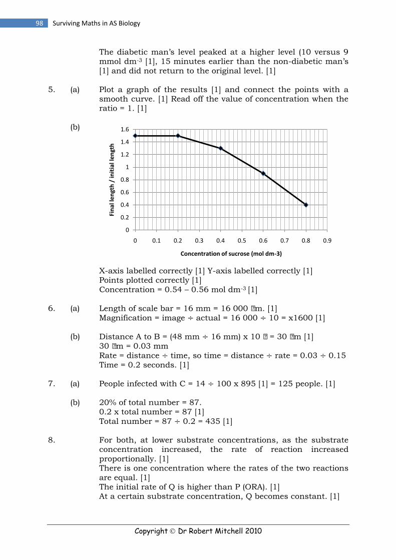
Copyright Dr Robert Mitchell 2010
98 Surviving Maths in AS Biology
The diabetic man’s level peaked at a higher level (10 versus 9 mmol dm-3 [1], 15 minutes earlier than the non-diabetic man’s
[1] and did not return to the original level. [1]
5. (a) Plot a graph of the results [1] and connect the points with a smooth curve. [1] Read off the value of concentration when the ratio = 1. [1]
(b)
X-axis labelled correctly [1] Y-axis labelled correctly [1] Points plotted correctly [1]
Concentration = 0.54 – 0.56 mol dm-3 [1]
6. (a) Length of scale bar = 16 mm = 16 000 µm. [1]
Magnification = image ÷ actual = 16 000 ÷ 10 = x1600 [1]
(b) Distance A to B = (48 mm ÷ 16 mm) x 10 µ = 30 µm [1]
30 µm = 0.03 mm
Rate = distance ÷ time, so time = distance ÷ rate = 0.03 ÷ 0.15
Time = 0.2 seconds. [1]
7. (a) People infected with C = 14 ÷ 100 x 895 [1] = 125 people. [1]
(b) 20% of total number = 87. 0.2 x total number = 87 [1]
Total number = 87 ÷ 0.2 = 435 [1]
8. For both, at lower substrate concentrations, as the substrate concentration increased, the rate of reaction increased
proportionally. [1] There is one concentration where the rates of the two reactions
are equal. [1] The initial rate of Q is higher than P (ORA). [1] At a certain substrate concentration, Q becomes constant. [1]
0
0.2
0.4
0.6
0.8
1
1.2
1.4
1.6
0 0.1 0.2 0.3 0.4 0.5 0.6 0.7 0.8 0.9
Fin
al le
ngt
h /
init
ial l
en
gth
Concentration of sucrose (mol dm-3)

Copyright Dr Robert Mitchell 2010
99 Dr Robert Mitchell
9. (a) Image width = 18 mm = 18 000µm
Actual width = image ÷ magnification [1]
= 18000 ÷ 12000
= 1.5µm [1]
(b) 1 mm = 1000 µm.
Number = 1000 ÷ 1.5 [1] = 667 [1]
10. (a) Ratio = 22.4 ÷ 22.2 [1] = 1.01 [1]
(b) It allowed the results to be compared, [1] because the masses of
the pieces of pear were different. [1]
(c) Plot of graph (ratio on y-axis, concentration on x-axis) [1] and
read off the concentration when ratio = 1. [1]
11. (a) Ѱcell = Ѱs + Ѱp
(b) Cell Ѱcell (kPa) Ѱs (kPa) Ѱp (kPa) A – 500 – 1000 + 500 B – 200 – 800 + 600 C – 400 – 1100 + 700
(c)
12. (a)
0
10
20
30
40
50
60
70
80
90
100
0 1 2 3 4 5 6
Cat
alas
e a
ctiv
ity
(%%
Iron (ii) nitrate / mol dm-3 x10⁻³

Copyright Dr Robert Mitchell 2010
100 Surviving Maths in AS Biology
x-axis labelled correctly. [1] y-axis labelled correctly. [1]
Points plotted correctly. [1] Smooth curve through points. [1]
(b) Draw line across from 50% to curve and down to x-axis. [1]
2.8x10⁻³ mol dm-3 [1]
13. (a) Over the first 15 seconds the breathing rate increases with an
increasing gradient, [1] after 15 seconds the heart rate remains
relatively constant at 83-84 bpm. [1]
(b) % increase = ((84 – 74) ÷ 74 ) x 100 = 13.5%
14. Inage length = 17 mm = 17 000 µm
Magnification = image ÷ actual = 17 000 ÷ 0.5 = 34 0000
15. (a) ( 1.24 + 1.32 + 1.28 + 1.29 ) ÷ 4 [1] = 1.28 seconds (3 sig fig) [1]
(b) Heart rate = 60 ÷ 1.28 = 46.9 beats per minute [1]
16. (a) Adenine Cytosine Thymine Guanine
Human 30.8 19.9 30.8 19.9
Chimpanzee 27.2 22.8 27.2 22.8
Shrew 26.7 23.3 26.7 23.3
Allow [1] per correct pair.
(b) Both mammals have a ratio of A:T and C:G of 1 [1]
The shrew has 0.5% less A and T and 0.5% more C and G than
the chimpanzee [1] ORA
17. (a) Over the five years, the peak flow increased steadily from approximately 260 to 320 with a decreasing gradient. [1]
(b) Any three of ... Both showed an increase in peak flow over the study. [1] The increase was steadier for the non-smoker. [1]
The maximum peak flow achieved by the smoker was less than the non-smoker. ORA [1].
The smoker had a lower start peak flow than the smoker. [1] One of the marks is for a relevant use of figures [1]
18. (a) 75% decline means the numbers were 25% of original. 25/100 x original = 140 000, hence:
Original = ( 140 000 x 100 ) ÷ 25 [1] = 560 000 [1]
(b) % increase = (( 580 000 – 140 000) ÷ 140 000 ) x 100 = 314%

Copyright Dr Robert Mitchell 2010
101 Dr Robert Mitchell
(c) Number of seals increased by 580 000 – 140 000 = 440 000
seals. [1] over 20 years, so rate = 440 000 ÷ 20 = 22 000 seals per year. [1]
19. Plant species Number of plants n(n-1)
Mat grass 10 10 x 9 = 90 Heath bedstraw 9 9 x 8 = 72
Bell heather 4 4 x 3 = 12 Sheep’s sorrel 2 2 x 1 = 2
Ling 3 3 x 2 = 6 Heath rush 14 14 x 13 = 182
Bilberry 1 1 x 0 = 0 Total = 43 ∑ n(n-1) = 364
= 4.96
20. (a) The standard deviations of the day zero groups were smaller
than at day 90 [1] showing the spread of data was larger at day
90 than at day 0. (ORA) [1]
(b) Control = 128% [1] A = 97.1% [1] B = 128% [1] A&B = 24.1% [1]
(c) Any four of ...
The tumours grew on all treatments. [1] In the absence of drug the tumours increased by 128%. [1]
Drug A reduced the growth of the tumours by about 30%. [1] Drug B alone had no effect on the growth of the tumours. [1]
The combination of drugs A and B caused a larger decrease in the growth of the tumours than the drug on their own.[1]
21. (a) Number of amino acids = 2 (antennae) x 12 000 (filaments) x 400 [1]= 9 600 000 [1]
(b) Bases on DNA = 3 x 400 = 1200 [1]
22. (a) A percentage allows a comparison [1] because the initial values of cholesterol were different in each man. [1]
(b) Both drugs caused a decrease in TC and LDL and an increase in HDL [1]

Copyright Dr Robert Mitchell 2010
102 Surviving Maths in AS Biology
Drug A decreased TC and LDL to a greater extent than B (ORA) [1].
Drug A increased HDL more than drug B (ORA). [1]
(c) Only six men were used. [1] No standard deviations are shown so no idea about spread. [1] There’s no information about how the men were controlled, e.g.
ages boss mass index, diet etc. [1]
23. (a) The number of cases of colon cancer increases with age for both
men and women. [1] In each age group there are more cases for men than women
(ORA). [1] Manipulation of figures, e.g. in the 20 – 44 age group women have a 50% lower incidence of the disease than men. [1]
(b) % increase = (( 300 – 120 ) ÷ 120 ) x 100 [1] = 150% [1]
(c) At age 32 her risk is 25 / 100 000 = 2.5x10⁻⁴ [1]
At age 87 her risk is 260 / 100 000 = 2.6x10⁻³ [1]
Increase in risk is 2.6x10⁻³ ÷ 2.5x10-4 = x10.4 [1]
Accept increase in risk = 2.6x10⁻³ – 2.5x10-4 = 2.35x10⁻³ [1]
(d) The data show that risk of colon cancer is correlated with age. [1]
The do not show that age causes colon cancer. [1]
24 Any three of ... Over the first two weeks of treatment the concentration of
phenylalanine decreased steadily [1]. It remained constant between
weeks 2 to 3 [1] and then started to rise again by week 4 [1]. Figures. [1]
25. (a) ERRATUM: The graph x-axis should read seconds. Common point = 1.28 – 0.6 = 0.68 seconds [1]
Heart rate = 60 ÷ 0.68 = 88 beats per minute [1]
(b) 88 beats per minute = 60 x 88 [1] per hour = 5280 [1]
(c) Cardiac output = heart rate x stroke volume [1] Cardiac output = 88 x 150 = 13 200 cm3 per minute [1] = 13.2 dm3 per minute [1]
26. (a) Vitamin C content decreased (from 2.5 g/100 g) with time. [1]
The gradient became less steep as time passed. [1] The vitamin C content remained approximately constant (at 0.25 g / 100g) after 3 weeks. [1]
(b) % decrease = (( 2.5 – 1 ) ÷ 2.5 ) x 100 [1] = 60.0% [1]

Copyright Dr Robert Mitchell 2010
103 Dr Robert Mitchell
27.
Prophase Metaphase Anaphase Telophase
Number of cells 15 6
60- (15+9+30)
9 30
% of cells in stage 25 10
6 ÷ 60 x 100
15 50
30 ÷ 60 x 100
Degrees on pie chart 90 36 54
15% x 360
180
50% x 360
28. (a)
x-axis labelled correctly [1] y-axis labelled correctly [1]
points plotted correctly [1] line of best fit appropriately placed [1]
(b) As the sodium phosphate concentration increased from 0 to 0.1 mmol dm-3 the growth of the seedlings increased proportionally [1].
(c) Any one of ...
The line of best fit does not go through the origin. [1] When phosphate is not present, there is still some growth. [1] There is scatter about the line. [1]
(d) Any one of ...
More data points (particularly between 0.06 and 1). [1] Repeat several times and take the average. [1] Increase the length of time the seedlings grew. [1]
29. The replication rate (in cycles per week) is: B 10
Hours per week = 24 x 7 = 168
Number of cycles = 168 hours ÷ 16.8 = 10
0
0.1
0.2
0.3
0.4
0.5
0.6
0.7
0.8
0.9
1
0 0.02 0.04 0.06 0.08 0.1
Gro
wth
(m
m in
2 w
ee
ks)
Phosphate concentration (mmol dm-3)

Copyright Dr Robert Mitchell 2010
104 Surviving Maths in AS Biology
30. The average width of one cell is: A 4 µm
2 mm = 2000 µm 2000 µm ÷ 500 = 4 µm
31. The picture in the book was: A 10 cm
Image size = actual size x magnification
Image size = 10 x 10 000 = 100 000 µm = 100 mm or 10 cm
32. (a) The growth rate was: B 1 mm day-1 (mm per day)
3.5 cm = 35 mm Growth was 35 – 2 = 33 mm in 33 days, so 1 mm per day.
(b) % increase was: C 1650%
% increase = ((35 - 2) ÷ 2) x 100 = 1650%
33. (a) Mean = C 12.6
Mean = (5 + 18 + 14 + 14 + 10 + 12 + 14 + 19 + 11 + 9) ÷ 10
(b) Mode = B 14 14 appears most frequently
(c) Median = B 13 Rank 5 9 10 11 12 14 14 14 18 19
Central numbers are 12, 14 the average of which is 13
(d) A TRUE B TRUE C TRUE Accurate, precise, valid, you name it, the conclusion was it!

Copyright Dr Robert Mitchell 2010
105 Dr Robert Mitchell
Glossary of HSW terms
Term Explanation
Accurate A measurement that is close to the true value.
Anomalous data Measurements that fall outside of the normal or expected range of
measured values. Biological variation makes identification of
anomalous values difficult, but sampling large numbers allows them
to be identified more easily.
Causal link, or
causation
A change in one variable that results from (or is caused by) a change
in another variable.
Chance The result of an investigation could have a genuine scientific
explanation or be due to chance. Scientist use statistical tests to
assess the probability that a result is due to chance.
Correlation A correlation shows a relationship between two variables. Evidence
of correlation does not automatically imply causation.
Dependent variable The variable measured for each change in the independent
variable.
Errors Errors cause a reading to differ from the true value.
Evidence Data or observations that are used in support of a hypothesis or belief.
Fair test A test in which only the independent variable has been allowed to change the dependent variable, i.e. one where all other variables are controlled.
Hypothesis A possible explanation of a problem that can be tested experimentally.
Independent variable The variable that is changed by the investigator. Null hypothesis A hypothesis that is worded in terms of there being no difference
or association (the negative version of a hypothesis). Precision Precise measurements are ones which have little spread about the
mean value. Probability The likelihood of an event occurring. It is different from chance
because it can be expressed mathematically. Random distribution These arise as a result of chance. Data will only be valid if collected
randomly as this avoids bias and allows a statistical testing. Reliability The ability to repeat the results of an investigation. Reliability can
be improved by taking more measurement or repeating the experiment many times.
True value The accurate true value that can be found if measurements are taken with no errors.
Validity Data are valid if they are made by the effect of a single independent variable.
Valid conclusion A conclusion that can be drawn if supported by reliable data measured by precise instruments to an acceptable degree of accuracy.

Copyright Dr Robert Mitchell 2010
106 Surviving Maths in AS Biology
Index
Copyright Dr Robert Mitchell 2010
107 Dr Robert Mitchell
Other books by CT Publications All our lovely books are available from www.ctpublications.co.uk

Copyright Dr Robert Mitchell 2010
108 Surviving Maths in AS Biology