Embed Size (px)
Citation preview

;£,_=!'-■» Cu4S;lFiCA'!C^ 3^ '«li PAGE 'tfhen Dm:a Entered)
REPORT DOCUMENTATION PAGE I . REPORT SUMBER 2. GOVT ACCESSION NO.
i TITLE fand Sublllle)
Detection in Inconpletely Characterized Colored
Non-Gaussian Noise via Parametric Modeling
■7. AUTHOR^J;
Steven Kay and Debasis Sengupta
9 PERFORMING ORGANI ZATiON NAME AND ADDRESS
Electrical Engineering Department University of Rhode Island Kingston, Rhode Island 02881
READ INSTRUCTIONS BEFORE COMPLETING FORM
3. RECIPIENT'S CATALOG NUMBER
5 TYPE OF REPORT i PERIOD COVERED
August 1984 to July 1986
6 PERFORMING ORG. REPORT NUMBER
8. CONTRACT OH GRANT NUMBERfJ)
N00014-84-K-0527
'0 PROGRAM ELEMENT. PROJECT, TASK AREA 4 WO«K UNIT NUMBERS
II CONTROLLING OFFICE NAME AND ADDRESS
Office of Naval Research Department of the Navy, Arlington, Virginia 22217
U MONITORING AGENCY NAME & ADDRESSr/' dlllcrem Irom ControlKng 01 lice)
12. REPORT DATE
August 1986 '3. NUMBER OF PAGES
33 15. SECURITY CLASS, (ol lh/» report)
Unclassified
I5» OECL ASSI Fic ATION DOWNGRADING SCHEDULE
16 DISTRIBUTION S^A-EMEN" -ol :hts Report
Approved for public release. Distribution unlimited.
17. DISTRIBUTION STATEMENT (ol the tbslraci entered /n Black 20, II dlllereni Irom Report)
18 SUPPLEMENTARY NOTES
19 K- E V WORDS 'C ■-.f.'.iur )n rrversr: iidc ■/ rrci-ssan- and I dentils- bv block numb or)
Non-Gaussian Processes Generalized Likelihood Ratio Itests Uniformly Most Powerful Itests
Erevdiitener-Gorre lator Autoregressive Processes Signal to Noiae Ratio
20 ABSTR AC ' 'C .f: f l.iue or^ reverse ^ide t{ necejaary and IdenUly bv block numborj
L
The problem of detecting a signal known except for airplitude in incorpletely characterized colored non-Gaussian noise is addressed. The problem is formulated as a testing of hypotheses using parametric models for the statistical behavior of the noise. A generalized likelihood ratio test is employed. It is shown that for a syrtinetric noise probability density function the detection performance is asymptotically equivalent to that obtained for a detector designed with a priori knowledge of the noise
DD IJAN73 1473 t-:):TIONOFlNCV65lSOBSOLETE
SECURITY CLASSIFICATION OF TMlS PAGE (Whan Dale Sntarma,

LtBRARY RESEARCH REPORTS DIVISION NAVAL POiiQRADUATE SCHOO.C MOKTEREY, CALIFQRHIA 93Q40,
Report Number 5 ^
t ^tection m Incompletely Characterized Colored Non-Gaussian Noise
via Parametric Modeling ,
STEVEN KAY AND DEBASIS SENGUPTA
Department of Electrical EkigLneering University of Rhode Island (Iruoi^^.^,
Kingston, Rhode Island 02881
1
\
^Sfti
August 1986
Prepared for
OFFICE OF NAVAL RESEARCH Statistics and Probability Branch
Arlington, Virginia 22217 under Contract N00014-84-K-0527 S.M. Kay, Principal Investigator
Approved for public release; distribution unlimited

Abstract
The problem of detecting a signal known except for amplitude in incompletely
characterized colored non-Gaussian noise is addressed. The problem is formulated
as a testing of composite hypotheses using parametric models for the statistical
behavior of the noise. A generalized likelihood ratio test is employed. It is shown
that for a symmetric noise probability density function the detection performance
is asymptotically equivalent to that obtained for a detector designed with a priori
knowledge of the noise parameters. Non-Gaussian distributions of the noise are
found to be more favorable for the purpose of detection as compared to the Gaussian distribution.

I. Introduction
The theory of detection of a known signal in presence of Gaussian noise having
a known covariance matrix is well developed [Van Trees 1968]. In many applications,
however, the covariance matrix is not known a priori. This difficulty can be alleviated
by characterizing the correlation pattern of the noise by a simple model and using
estimates of the model parameters to design a detector [Whalen 1971], [Bowyer et al
1979], [Kay 1983]. The difficulty increases when full information regarding the noise
probability density function (PDF), usually assumed to be Gaussian, is unavailable
due to insufficient knowledge about the noise source [Knight et al 1981]. There is no
uniformly most powerful (UMP) test in this case because the use of a Neyman-Pearson
criterion leads to a detector which depends on the unknown parameters. The Bayesian
method of assigning priors to the unknown parameters of the noise PDF produces an
'optimal' detector [Lee et al 1977], but requires a multidimensional integration. Its
performance is critically dependent on the accuracy of the choice of priors. A robust
detector [Kassam and Poor 1985], on the other hand, does not use any partial knowledge
about the noise PDF and therefore is not expected to perform well. Locally optimal
(LO) detectors for this problem have been studied extensively by Czamecki, Martmez,
Thomas and others [Czarnecki and Thomas 1984], [Martinez and Thomas 1982]. Their
results however rely on a known covariance matrix and marginal PDF of the noise. A
third dimension is added to the problem if the amplitude of the signal is not known
[Kay 1985]. A locally optimal detector can not be used since it depends on the polarity
or sign of the amplitude, which is usually unknown.
This paper addresses the problem of detecting a deterministic signal known except
for amplitude in the presence of incompletely characterized non-white non-Gaussian
noise. The approach chosen here is to use the theory of the generalized likelihood ratio
test (GLRT) for composite hypothesis testing [Kendall and Stuart 1979]. The work
presented here is an extension of the work of Kay [1985] in which the noise is assumed
2

to be non-Gaussian but white. In this case the covariance matrbc is assumed to be
known except for a few parameters. Maximum hkelihood estimates (MLE) for these
parameters are then used in the GLRT. The asymptotic performance of the GLRT
detector is shown to be equivalent to the asymptotic performance of the clairvoyant
GLRT detector (one which uses perfect knowledge of the unknovra parameters) for a
symmetric noise PDF. Therefore the GLRT asymptotically achieves an upper bound
in performance and is optimal in this sense.
The paper is organized as follows. Section 11 gives the theory of the GLRT which
will be used extensively in the subsequent sections. Section III formulates the detec-
tion problem and derives the GLRT for it. The case of autoregressive (AR) noise is
considered separately. Section IV discusses the performance of the GLRT detector and
compares it to that of the clairvoyant GLRT detector. Section V draws some general
conclusions about the performance of the GLRT . Section VI summarizes the results
and discusses the implementation aspect of the problem.
n. Review of Generalized Likelihood Ratio Itest
Consider the problem of testing the value of the parameter 0 = [0^ Qj] ^ based
on the a data set y = [yi y2 • • • VN]. ©r and 0^ are assumed to be vectors of dimension
r and s, respectively. A common hypothesis test is
. ;/o: e^ = [0^ 0f ]
;/i : 0^ = [0^ 0f ] 0.^0 ^^^
0«, referred to as the vector of nuisance parameters, is of no concern and may assume
any value. Assuming the observed data y has a joint probability function f(y; 0^, 0^),
a generalized likelihood ratio test for testing (1) is to decide ^i if
f(y;Q„e.) ° f(y;o,e,) *^ <''
for some threshold 7. 0 is an r-dimensional vector of zeroes. Q^ is the MLE of 0^
assuming )^o is true while 0^ and 0, are joint MLE's of 0^ and 0^ assuming Mi is

true. 03 is found by maximizing f(y;O,03) over G^. Similarly, 0„ ©3 are obtained
by maximizing f(y; 0^,03) over 0^ and 03.
The statistics oi ic are difficult to obtain in general. For large data records (asymp-
totically) it may be shown that 21n£G is distributed in the following manner [Kendall
and Stuart 1979].
2In£G~Xr
21n£G~x"(r,A)
under ^0
under ^1
(3a)
(36)
Here Xr represents a chi-square distribution with r degrees of freedom and x''^{r,X)
represents a noncentral chi-square distribution with r degrees of freedom and noncen-
trality parameter A. Note that x'^(r,0) = xl or the distribution under ;/o is a special
case of the distribution under )ii and occurs when A = 0. The noncentrality parameter
A, which is a measure of the discrimination between the two hypotheses, is given by
A = 0?- [le.e, (0,0.) - le.e. (0,0,)I-,^e. («> 0a)l|.e. (0,0.)] 0r (4)
where 0^, 0« are the true values. The terms in the brackets of (4) are found by
partitioning the Fisher information matrbc for 0 as
'le.e.(0r,0«) le.e.(0r,0a) 1(0) =
^l©.e.(0r,0.) Ie.e.(0r,0a) (5)
and the partitions are defined as
d\ni\fd\ntY dQr ) \ dQr
le.e.(0.0.)=^^(^^j(^—^
Ie.e,(0r,03)=li^e.(0r,0.)
le.e.(0r,0a) =E ' ^' ^ dQ, dQ.
r xr
r X s
s xr
s X s (6)

All the paxtitions of the Fisher information matrix are evaluated at 0^ = 0 and the
true values of 03 for use in (4).
The motivation for using a GLRT is that for large data records it exhibits certain
optimality properties. A uniformly most powerful (UMP) test does not exist in many
situations. However, of all the tests which are invariant to a natural set of transfor-
mations the GLRT exhibits the largest probability of detection. The GLRT is said to
be the asymptotically uniformly most powerful invariant (UMPI) test [Lehmann 1959].
It is also a consistent test in the sense that the probability of decidmg MQ when Mi is
actually true approaches 0 for large data records. Asymptotically the GLRT is unbi-
ased, i.e., the probability of detection when )li is true is larger than the probability
of false alarm. (This result follows from (3) and properties of the chi-square distribu-
tion.) Finally, although the GLRT does not usually exhibit a constant false alarm rate
(CFAR) it does so for large data records. It is difficult to find the conditions under
which the asymptotic results apply to finite length data records. The following heuristic
conditions follow from [Cox and Hinkley 1974].
1) The asymptotic statistics of the MLE's used m the likelihood ratio should
be applicable, i.e., they should be Gaussian with mean equal to the true
parameter value and covariance matrix equal to the inverse of the Fisher
information matrix.
2) The two hypotheses should be reasonably close and only slight departures of
©r from zero should be tested.
ni. Formulation of the Problem and GLRT Solution
The detection problem considered here is the following.
;/o:y = Wu (7)
)/i : y = Wu + )us
where s = [^i 52 • • • SN]"^ is a vector of known signal amplitudes, u = [ui U2 • • • UN]'^
5
is a vector of independent and identically distributed [i.i.d.) noise with a symmetric
PDF, /x is an unknown scalar (either positive or negative) and W is an invertible
(TV X A'') matrix whose elements are functions of a set of unknown parameters ^ =
[W].y=W,,(^)
Since Un, n = l,2,---N are i.i.d., the PDF of u can be expressed as
N
f(u;$) = []/(un;$) (8) n=l
where /(u„; $) is the margmal PDF of each u„ dependent on the unknown parameter
vector $. / is assumed to be symmetric, i.e., f{-u) = f{u). Note that the covariance
matrix of the noise is a^WW^ where a^ is the variance of u^.
(7) represents a general set of problems. The unknown matrix W allows for a
large class of spectral characteristics or correlation patterns of the background noise.
For large data records autoregressive (AR), moving average (MA) and autoregressive
moving average (ARMA) processes can be represented by the above formulation of the
underlying random process if W is the impulse response matrbc of the corresponding
filter. Secondly, the PDF of Un can be chosen to characterize specific problems in a
realistic way. The parameter vector $ is left unknown in order to add Bexibility to the
noise PDF model. Thirdly, by allowing n to be positive or negative the detector will
be able to accommodate a change of polarity in the signal.
The problem of (7) can be recast as
;/o : 0^ = [0^ Gf] (9a)
: ; ;/x : 0^ = [0^ 0^ 0.7^0 , (96)
where ©r = M a scalar
0a = [^ $ ] (vector of nuisance parameters)
6
(10)

Since (9) is equivalent to (l), the GLRT for testing Mi vs. )^o is given by (2). In
order to evaluate the MLE's it is necessary to find the joint PDF of y under either
hypothesis which can be found from the joint PDF of u in the following way. From (7)
it follows that
u = W-V under MQ (lla)
u = W-i(y-/is) under )ii (ll6)
W-^ exists because W is assumed to be invertible. The elements of W^ are also
knovm fimctions of ^.
l'^-%=^vm (12)
(11) bemg an affine transformation, the joint PDF of y can be written as
under MQ u=W-iy
under Vi u=W-i(y-M8)
j under }IQ (13a)
which m view of (8) and (U) reduces to
'(^'*'^)=Mw)in(^^^"'^^
^^^'^'^^=Mi^n(/("-^) ^, \undern, (136)
Therefore the GLRT for this problem is to decide ^/i if
N / N ^ ^\
, n=l \j = \ ^ ^^- ^7-lv N >^ (14)
1=1 VJ = I /
where hat's denote MLE under )lo and double hat's denote MLE under Mi. It is assumed
that the values of |det(W)| under HQ and Mi axe nearly the same. This assumption
7
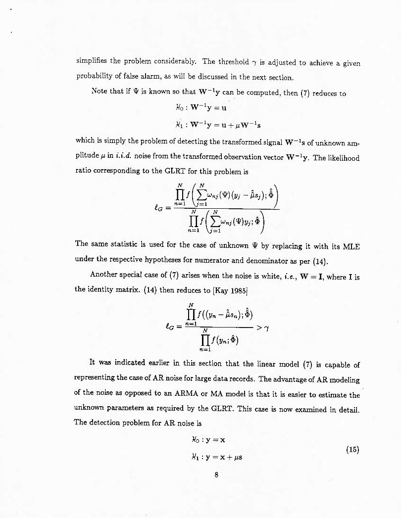
simplifies the problem considerably. The threshold 7 is adjusted to achieve a given
probability of false alarm, as will be discussed in the next section.
Note that if * is knovra so that W"-V can be computed, then (7) reduces to
;/o:W-V = u
which is simply the problem of detecting the transformed signal W-^s of unknown am-
plitude n in i.i.d. noise from the transformed observation vector W'^y. The likelihood
ratio corresponding to the GLRT for this problem is
N / N
Xlf\jynjm{yi-hsj)-,^ n=l VJ = 1
ta = N / N
fl/ E'^ny(*)y;;$
The same statistic is used for the case of unknown * by replacing it with its MLE
under the respective hypotheses for numerator and denominator as per (14).
Another special case of (7) arises when the noise is white, ».e., W = I, where I is
the identity matrix. (14) then reduces to [Kay 1985]
N
J{f{{yn-hn)-A) B n=l to j^ > 7
n=l
It was indicated earlier in this section that the linear model (7) is capable of
representing the case of AR noise for large data records. The advantage of AR modeling
of the noise as opposed to an ARMA or MA model is that it is easier to estimate the
unknown parameters as required by the GLRT. This case is now examined in detail.
The detection problem for AR noise is
)/o : y = X
(15) . ^1 : y = X + )us
8

with
X = [xi X2 ■■■ XN^
It is assumed that the sequence {xi,X2, • • ■,XN} is the output of a pth order all-pole
filter excited by white driving noise or
p
alternately,
Un-Xn+'^ ajXn-j = ^^ajXyi-j, n = 1,2, • • • iV y=i y=o
assuming OQ = 1. u„ can also be written as a function of y under either hypothesis
Un = ^ajyn-j, n = 1,2, • • • iV under MQ (16a)
under Mi
y=o p
^oy(y„_y-^s„_y), n = l,2,---iV y=o
(166)
Note that ui, U2, •■■ Up involves samples prior to yi which are outside the observation
interval. These are assumed to be zero for simplicity. For large data records this
assumption will not change the character of the GLRT. In the matrix form
/ ui \ /I
Un
«p+l
Or
0 a.
\ / yi-fiSi \
Vp+i - iJ.Sp+1 (17)
\ UN J \0 ... 0 ap ... Ij \ y^-f^sN J
under ^i. The equation is the same under MQ, except that /x = 0. (17) is a special case
of (11) with * = a = [ai 02 • • • Cp] and M = p. W-^ is a lower triangular Toeplitz
matrix given by ro, ifi<j,
w,y(a) = <^ Oi_y, ifj<t<y + p, I 0, if j + p < i.
9

To avoid having to assume that {y-(p_i), y-(p-2), ■ ■ •, yo} are zero one can proceed
as follows. Considering only the last [N - p) equations of (16) which expressed in the
matrix form are
/ "p+i \ / 1
«2p «2p+l 0 a-
\ UN J V 0 0 a.
\ / Vp+l - M5p+1 \
y2p - M-S2p y2p+i - ^J'S2p+l
Ij V VN - fJ-SN J
+
^Op_y+i(yy-^5j)
P
X]°P-J+2(yj-M5;) y=2
<»p(yp-M-Sp) 0
(18)
under )^i. Substitution of /^ = 0 in (18) gives the corresponding equation for UQ.
(18) is also a special case of (lib) except that only the last {N - p) of the N scalar
equations implied by (lib) are used. Smce the added vector causes a departure from
the general model, the previous results can not be used. To determine the GLRT first
consider the conditional likelihood function. In this case the conditional likelihood of
yp+i,yp+2,-",yiV given yi,y2,---,yp is .
f (yp+i > yp+2, • • •, yiv |yi, y2, ■ • •, yp)
N
n / &yn-;;$ n=p+l \j=0
N / p
" n / &(y''-J-M5n-;);$ n—p+l \y=o
under ^o
under )ii
(19a)
(196)
10

The likelihood ratio is given by
£^ ^ f(yp+i>yp+2,• • •,yjvlyi,y2, • • •,yp;Qr,Qa) f(yi,t/2,• • •,yp; Qr,Q3)
f(yp+i,yp+2,---,y7v|yi,y2,---,yp;O,0,) f{yuy2,---,yp;0,Qs)
n=p+i V;=o N
n / Z^^yy"-;-;^ n=p+l VJ=0 y
f(yi)y2,---,yp;A,a,<^
f(yi>y2,---,ypiO,a,$
A
where OQ and CQ are defined to be unity. The second term is dropped for ease of
computation. A heuristic justification for ignoring the second term is that when N is
large, its contribution to IQ will be negligible. The closer the poles of the AR model
to the unit circle, larger is the requirement for N [Box and Jenkins 1970], [Kay 1981].
With this simplification, the GLRT decides )^i if
p
iG =
N
n=p+l \j=0 N
n /(&yn-y;^ n=p+l
>7 (20)
A comparison of (14) and (20) shows that the latter uses fewer terms in the product.
However both formulations are clearly asymptotically eqivalent. Figure 1 is a block
diagram to generate 2 hi£G from the data. The reason for computing 2 In^c instead of
IG will be clear from the discussion in the next section. The block diagram is very much
similar to that obtained by [Kay 1983] for the detection of a completely known signal
in unknown colored Gaussian noise. In the Gaussian case In / is a simple quadratic,
while for the general non-Gaussian case it will be highly non-linear. Figure 1 also uses
an estimator for fi which was assumed to be known hi [Kay 1983].
rV. Asymptotic Performance of the GLRT Detector
Asymptotic distributions of 2 In IG under )^o and Mi are given by (3a) and (36)
respectively. In this case 0, = /z, 0, = [^^ $^]r for the general linear model and
11

©3 = [a^ $^]^ for the AR case. Hence the noncentrality parameter is
A = M' [W(0, O.) - I^e, (0, G3)Ie,'e. (0, O^jlje. (0,0,)] (21)
The probabiUty of false alarm is
PFA = P{2lniG>i'\)^o} (22)
where 7' = 2 In 7. The probability of detection is
PD = P{2\niG>l'\Mi} (23)
Both the probabilities can be calculated from the tables of noncentral and central chi-
squared distributions, respectively. In practice, 7' can be set to produce a given false
alarm rate and P© can be calculated from (23) accordingly.
As indicated before, there is no UMP test for the detection problem considered in
this paper. Therefore there is no upper bound to which the performance of any detector
may be compared. However the performance of the GLRT is better appreciated when
compared to that of a clairvoyant GLRT. A clairvoyant GLRT is one which uses perfect
knowledge of the nuisance parameters Qg. The likelihood ratio in this case is
g,,_f(y;Qr,Q3)
"""^ f(y;o,0.)
which in view of (13) is
N / N
toe = ^^ y
n/(E'^ny(^)yy;*
where ^ and $ are assumed to be known. Asymptotically, 2 In £GC is distributed as
2b£GC~Xr under ;/o (24a)
2]niGc-x'^r,\,) under ;/i (246)
12

where .
Ae = 0,^Ie.e.(O,03)0r
For the problem considered here, r = 1 and Qr = /J,. Hence
Ae = M^/^^(O,03) (25)
Comparing A and A^ as given by (21) and (25), respectively, it is apparent that A is
equal to A^ less an additional term. Assuming that IQ^Q is positive semidefinite,
Ac>A
From the theory of noncentral chi-square distribution it can be shown that P^ as given
by (23) is a monotonic function of the noncentrality parameter, which implies that PD
for the clairvoyant GLRT is greater than or equal to that for the GLRT [Sengupta
1986]. Therefore the clairvoyant GLRT detector, although impractical in this case,
provides an upper bound on the performance of the GLRT detector. In order that the
upper bound be achieved, A should be equal to Ac. This will occur if
lMe.(O,0,)=O . (26)
Appendices A and B show that this is indeed the case for the general Imear model of
(7) and the AR noise model of (15), respectively, if as assumed / is a symmetric PDF.
Therefore the asymptotic performance of the GLRT is equivalent to the performance
of the clairvoyant GLRT for detection in presence on non-Gaussian noise modeled as
in (7) or (15). This implies that one can do as well in detecting a signad of unknown
amplitude as if the unknown noise parameters were known.
V. General Conclusions about the Performance of the GLRT
A key to the asymptotic performance of the GLRT detector is the noncentrality
parameter A, which is found to be equivalent to Ac. It would be interesting to examine
13

how A depends on the statistical properties of the noise. First consider
Uf^,Qs) =E ainf
N , N
= E
N
51n J]/K;$) vn=l
N
= E^ n=l
dpt
^ln/(u„;$)
2-t
using (116) and (12)
(27)
The last step follows from the facts that u„'s are i.i.d. and that the cross-terms are
zero, since
E dn ln/(u„;$)
5)U i;[ln/(u„;$)]=0
under certain regularity assumptions on / [Bickel and Doksum 1977]. Writing (116)
explicitly as N
J = l
it follows that
(28)
(29)
Hence (27) can be rewritten as
N
n=rl
AT
[fe^/(-*>)(|f
n=l
N a In/ 5Un
14

a^Ifi^) (30)
where a^ is the variance of u„ and
J/($) = E a In/
does not depend on /i or u„. The expectation is with respect to Un only smce Un's
j.j.d. It follows from (25) that
axe
A = A. = N N
1=1 \ j=i a2j/($)
= ^8^(W-^^W-^)sa2j/($)
= (MS^)(cr2wW^)-i(/.s)^c72j/($)
= S^R-lso[c72j^($)] (31)
where R = a^WW^ is the iV x iV autocorrelation matrix of the colored noise and
So = fis Is the signal vector including the amplitude. SJR-^SQ is the signal to noise
ratio (SNR) at the output of a prewhitener followed by a matched filter (or correlator),
both built with perfect knowledge of the filter parameters (*). To be more precise,
if the data is passed through an ideal whitener ( a filter which will completely whiten
the noise) and correlated (multiplied term-by-term and summed) with the output of
a similar filter through which only the known signal is passed then SJR-^SQ is the
15

squared ratio of the contributions from the signal and noise parts of the data. In the
case of AR noise, a similar derivation using (166) (instead of (28)) gives
n=p+l \ y=o (32)
and
A = M N
0-2 Z^ I / ^0-jSn-j n=p+l \ ;=o
a'lfi^) (33)
= ^(As)^(As)a2j^($)
where A is the (iV - p) x iV Toeplitz matrix
f a-p ... ci 1
0 Up ... d A =
0
1
\o 0 Qr
0\
■•• 0
ai Ij
Therefore
X = s^R-ho{a^If{^)] (34)
So = MS as before and R = ^^(A^A)-^ is approximately the covariance matrix of the
noise. Clearly, A is proportional to the SNR at the output of a prewhitener-correlator
(usmg true value of a) in the AR case also.
Having established similar results in the cases of AR noise and the general linear
model, an attempt is now made to examine them. The AR noise model is chosen for
this purpose because of its intuitive frequency-domain interpretation. Figure 2 is a
block diagram representing (33). It shows that A can be obtained by inverse filtering
the signal and summing the squares of the output of the filter, ff the signal has most
of its power at the frequency where the inverse filter has a zero, the output power and
hence A will be small leading to a small probability of detection. In other words, it
16

is difficult to detect the signal if the peaks of the signal spectrum coincides with the
peaks of the noise PSD. This makes perfect intuitive sense. On the other hand it is
possible to maximize A by choosing a suitable signal s for a given noise background.
This can be done by constraining the signal energy to be constant and maximizing the
SNR at the output of a prewhitener-correlator over all possible signal shapes. Writing
the Toeplitz matrbc R in terms of its orthonormal eigenvectors {vi, V2, • • •, vjv} and
eigenvalues {Ai, A2, •••, AN}
N
^ = EV>vJ (35) j=i
it follows that
Hence
^-' = th,-J 7—'Ay
s5-R-'so = f:-^{s„Sf
N
'Av = Eh^ (36)
where ?y = s^vy is the component of the signal SQ along the eigenvector Vy. The
condition of constant signal energy can be written as
8^So = P, (37)
Since the eigenvectors are orthonormal
"" N N N
E->-J .T So = S^ So = Pa (38)
The SNR given by the weighted sum (36) has to be maximized subject to constraint
that the unweighted sum of the squares is fixed at Pg as m (38). In general, R will
be positive definite and all the eigenvalues will be positive. If there exists a minimum
17

eigenvalue Kk, then the SNR is maximized by choosing <;k = -/Pj and ?y = 0 for
j i^ k, I.e., by choosing SQ to be proportional to v^. Since the probability of detection
given by (23) is a monotonic function of A which is proportional to the SNR at the
output of a prewhitener-correlator, the above choice of the signal shape for a given
signal energy also maximizes the probability of detection. If one of the eigenvalues A^
is zero, then it is possible to chose the signal in such a way that there is no component
of noise along the signal vector and therefore the SNR is infinite giving rise to singular
detection. Therefore the probability of detection is maximized by choosing the signal
in the direction of the smallest noise component. This is the discrete time equivalent
of a well-known result for the continuous case [Van Trees 1968]. An interesting special
case occurs when iV -> oo such that the eigenvectors become
Hence the optimum signal is a sinusoid in the direction of the eigenvector associated
with the minimum eigenvalue. For very large data records the eigenvalue Ay correspond-
ing to the eigenvector Vy approaches the value of PSD at the frequency /y. Hence the
signal easiest to detect would be a sinusoid at the frequency at which the noise PSD
has a minimum. This is also apparent from the frequency domain equivalent of (36)
(using Perseval's theorem)
0.5
where So{f) is the signal spectrum (Fourier transform of SQ) and Puu is the noise PSD.
With the constraint that
/
0.5 2 So{f)M = i
-0.5
which is equivalent to (37), the integral is maximized if the numerator is large only
where the denominator is small or zero. This result has a nice intuitive justification.
18

However if the filter parameters are completely unknown the above result can not be
used to select a suitable signal.
The next issue of interest is the effect of the noise PDF on the detection perfor-
mance. A reasonable basis of comparison should be formed for this purpose. Therefore
the Gaussian and non-Gaussian noise processes are assumed to have the same PSD,
i.e., the same spectral shape and power and detection of the same signal is considered.
Consequently, the comparison is done on the basis of a fixed signal to noise ratio (or
s^R~^so). Under these assumptions, the probability of detection is larger for that noise
PDF which has a larger value of a'^If. In other words, given two noise backgrounds
with the same PSD but different underlying noise PDF's, in order to achieve the same
probability of detection, more SNR is required for that background for which o'^If '.s
smaller. It is known that among all symmetric and integrable PDF's, the Gaussian
PDF is the only one for which a'^If attains its minimum value of unity [Sengupta and
Kay 1986]. Therefore for a given noise PSD, it is easier to detect a signal known except
for amplitude in non-Gaussian noise than in Gaussian noise. From (34) it follows that
in order to have the same noncentrality parameters in the non-Gaussian and Gaussian
cases
where SMZNG and S}/ZG are the SNR's requu-ed in non-Gaussian and Gaussian
noises, respectively, in order to achieve a given probability of detection {i.e., a given
A). The above equation can also be written as
^O^og,o^rjj±=lOlog,,{a'lf) (39)
Therefore 101ogio(cr^J/) is a measure of the SNR bonus in dB for a non-Gaussian
distribution. The result also holds for the special case of white noise when (33) becomes
A = .2JL
CT2J/($) (40) 2 ''
n=l
19

The quantity CT^JJ: is now shown to be independent of scaling. If the random
variable uhasa. PDF /(u) then the normalized random variable u = u/a has. the PDF
hence
"'"-'L
g{u) = cr/(u)
du f{u]
7-00 1 r«
/•OO
a2 -du
=/: g(u)
Hence cr^ J^ depends only on the shape of the PDF and is unaffected by scaling. There-
fore the SNR bonus quantified by (39) is the same for any value of the noise power as
long as the powers of the non-Gaussian and Gaussian processes are the same.
It is interesting to note that the same quantity represents the amount of departure
from Gaussianity for the problem of estimating AR filter parameters of a non-Gaussian
AR process. The OR bounds for these parameters are found to be less m the case of a
non-Gaussian PDF than the corresponding bounds in the Gaussian case by a factor of
o'^If [Sengupta and Kay 1986].
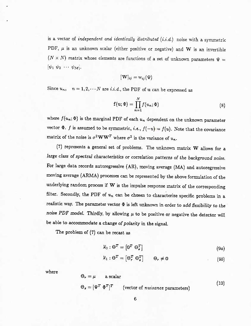
As an illustration of the improvement made by the proposed detector over the
Gaussian detector, consider the mixed-Gaussian noise PDF
The first term on the right hand side is referred to as the background component with
variance a| and the second term is called the interference component with variance
CTj. e is called the mixture parameter and is regarded as a measure of the degree of
20

contamination of the background Gaussian process by the interference process. The
model Is useful in representing a nonunally Gaussian noise background characterized by
the presence of sharp spikes or impulses [Sengupta and Kay 1986]. Assuming a% = 1
and aj = 1000, Figure 3 plots the SNR bonus given by (39) vs. e (in this case $ = e). It
shows how much improvement can be expected over the Gaussian case in terms of SNR
while detecting a signal known except for amplitude in colored noise. The comparison
is made, as indicated before on the basis of the same PSD m the Gaussian and mixed-
Gaussian cases. It should be mentioned, however, that introduction of impulses m an
otherwise Gaussian environment does not improve the probabihty of detection, which
is expected intuitively. This is because of the fact that introduction of impulses also
increases the noise power by a considerable amount. This increase in noise power is
alleviatedhy employing a non-Gaussian detector. As an example, for e = 0.1, the overall
noise variance is approximately 100<r| (as compared to a| before the introduction of
impulses), i.e., the noise power increases by 20 dB. It can be observed from Figure 3 that
the SNR bonus is also approximately 20 dB for e = 0.1. Therefore the mixed-Gaussian
detector does not suffer from a loss of performance unlike the Gaussian detector whose
threshold of detection is expected to go down considerably with the introduction of
impulses.
VI. Summary
The GLRT for the detection of a signal known except for amplitude in unknown
colored non-Gaussian noise was derived in section III through parametric modelmg of
the noise PDF and covariance matrix. The popular time series models such as AR,
MA and ARMA for the noise are asymptotically special cases of the proposed linear
model for large data records. The GLRT was found to achieve the performance of a
clairvoyant GLRT asymptotically, i.e., knowledge of the nuisance parameters is not
required to attam an upper bound in performance. The effects of the signal spectrum
21

and the noise PSD on the detection performance was discussed. It was observed that
it is difficult to detect a signal whose spectrum matches the noise PSD. If, however,
most of the signal is along a direction of low noise component, it is very easy to detect.
The asymptotic performance of the GLRT for Gaussian and non-Gaussian noise models
were compared. It was concluded that detection in non-Gaussian noise is easier than
detection in Gaussian noise for the same noise PSD. The improvement in performance
of the GLRT in a non-Gaussian noise background over the Gaussian case is easily
quantified in terms of the SNR 'bonus' as a function of the nobe PDF parameters.
In order to implement the GLRT described in section HI one needs to find the
MLE's of the unknown parameters under each hypothesis. Some work along this line
has been done for the case of AR noise [Sengupta and Kay 1986, 2], using reasonable
approximations to reduce computation. This work is approriate for estimation under
the null hypothesis {){i) and extension to the case of alternative hypothesis (Mi) is not
straightforward except for the special case of a d.c. signal {sj = 1, j = 1,2,-• • ,N).
Evaluating the joint MLE of the mean or the location parameter (/z) and the AR filter
parameters may be particularly difficult for most non-Gaussian processes. Computa-
tionally efficient approximations to the GLRT, such as the Rao test and the Wald test
[Rao 1973] can be used for this purpose. Estimation of the mean and the other param-
eters under Ui can thus be avoided for small signal amplitudes [Sengupta 1986]. This
problem will be addressed in a future paper.
References
[l] H.L. Van Trees, Detection, Estimation, and Modulation Theory, Chapter 4,
New York: John Wiley, 1968.
[2] A.D. Whalen, Detection of Signals in Noise, Chapter 9, New York: Academic,
1971.
22

[3] D.E. Bowyer et al, "Adaptive Clutter Filtering using Autoregressive Spectral
Estimation", IEEE Trans, on Aerosp. Electron. Syst., pp. 538-546, July 1979.
[4] S.M. Kay, "Asymptotically Optimal Detection in Unknown Colored Noise via
Autoregressive Modeling", IEEE Trans, on Acoustics, Speech and Signal Processing,
pp. 927-940, Vol. ASSP-31, Aug. 1983.
[5] W.C. Knight, R.G. Pridham and S.M. Kay, "Digital Signal Processing for
Sonar", Proc. of the IEEE, pp. 1451-1506, Nov. 1981.
[6] S.C. Lee, L.W. Noite and C.P. Hatsell, "A Generalized Likelihood Ratio For-
mula: Arbitrary Noise Statistics for Doubly Composite Hypotheses", IEEE Trans, on
Info. Theory, pp. 637-639, Vol. IT-23, Sept. 1977.
[7] S.A. Kassam and H.V. Poor, "Robust Techniques for Signal Processing", Proc.
of the IEEE, pp. 433-481, Vol. 73, Mar. 1985.
[8] A.B. Martinez and J.B. Thomas, "Non-Gaussian Multivariate Noise Models for
Signal Detection", ONR report #6, Sept. 1982.
[9] S.V. Czarnecki and J.B. Thomas, "Nearly Optimal Detection of Signals in Non-
Gaussian Noise", ONR report #14, Feb. 1984.
[10] S.M. Kay, "Asymptotically Optinial Detection in Licompletely Characterized
Non-Gaussian Noise", Submitted to IEEE Trans, on Acoustics, Speech and Signal
Processing, 1985.
[11] Sir M. Kendall and A. Stuart, The Advanced Theory of Statistics Vol. II,
Chapters 18-19, New York: MacMillan Publishing, 1979.
[12] E.L. Lehmann, Testing Statistical Hypotheses, New York: John Wiley, 1959.
[13] D.R. Cox and D.V. Hinkley, Theoretical Stastics, Chapter 4, London: Chap-
man and Hall, 1974.
[14] G.E.P. Box and G.J. Jenkins, Time Series Analysis: Forecasting and Control,
Chapter 7, San Francisco: Holden-Day, 1970.
[15] S.M. Kay, "More Accurate Autoregressive Parameter and Spectral Estimates
23

for Short Data Records", presented at the ASSP workshop on Spectral Estimation,
Hamilton, Onterio, Canada, Aug. 17-18, 1981.
[16] D. Sengupta, "Estimation and Detection for Non-Gaussian Processes using
Autoregressive and Other Models", M.S. Thesis, Dept. of Electrical Engineering, Univ.
of Rhode Island, 1986.
[17] RJ. Bickel and K.A. Doksum, Mathematical Statistics: Basic Ideas and Se-
lected Topics, Chapter 4, San Francisco: Holden-Day, 1977.
[18] D. Sengupta and S.M. Kay, "Efficient Estimation of Parameters for Non-
Gaussian Autoregressive Processes", submitted for review to IEEE Trans, on Acoustics,
Speech eind Signal Processing.
[19] S.M. Kay and D. Sengupta, "Simple and Efficient Estimation of Parameters
of Non-Gaussian Autoregressive Processes", submitted for review to IEEE Trans, on
Acoustics, Speech and Signal Processing.
[20] C.R. Rao, Linear Statistical Inference and its Applications, Chapter 6, New
York: John Wiley, 1973.
APPENDIX A
Asymptotic Optimality of the GLRT
for a General Linear Model of the Noise
Assuming that / is an even distribution and ©a is as given in (10), it will now be
shown that (26) holds for the detection problem defined ui (7). It suffices to prove that
I^i,{(x,^,^) = E
and
/;.*(/x,^,$)=i; d^
ahif\/ahf dfi )[ 6<if
'ainf\/ahf^
= 0 (Al)
(5$ 0 {A.2)
24
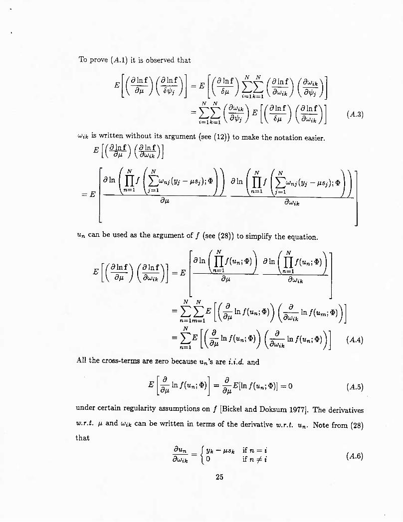
To prove (A.l) it is observed that
^ /(91nf\/(91nf dfj, J y 8%l)j
^E '<91nf\ Y^v-^ (d\nf\ fduik
•^/^ yferife v^^'W v<9V'; N N
ttt[ V di'j du>ik
E ainf\ /(91nf 6fj, J \ dtui
{A.3)
Uik is written without its argument (see (12)) to make the notation easier.
E r^akfWainf ofi J \ duj. ik J.
E
N ( N N I N
d^j, duik
Un can be used as the argument of / (see (28)) to simpUfy the equation.
E ainfX /ainf
dfx I \ dijJi = E
^in(n/("-*)) <91n(n/("-*) ,n=l >n=l
5^ a^iA
AT N
n=lm: ^ In/Ki^j'jf^ln/Cu™;*)
5/i . 5W,A
n=l |:hi/(u„;$)V^ln/(un;$)^ 5/x ,^W,A
(A.4)
All the cross-terms are zero because u„'s are i.i.d. and
E ^ln/K;$) = 5;^^[ln/(un;$)]=o (A.5)
under certain regularity assumptions on / [Bickel and Doksum 1977]. The derivatives
w.r.t. fj, and u;,fc can be written in terms of the derivative w.r.t. Un- Note from (28)
that
^"n _ [Vk- IJ-Sk if n = i dijjik 1 0 if n 7^ t (A.6)
25

From (A.6) and (29) it follows that (A.4) can be rewritten as
N
E d\ni\ /ainf
dfj, j \ dujik d\nf\ fdun\ /^ln/\ fdun dun J \ dfJ, J \ dUn J [duJik
N
^ In/(„,;*) Vk - (J-Sk
odd
odd
{Vk - ^tSk) is a linear function of u, as observed from (7). The PDF / is even and
expectation is taken on a function which is odd over each Un. Therefore the expectation
must be zero.
E dhd) fainf\i dfi J \duikj_
N
■^CJ.ySy E
J = l
N
■\2 f N
^ln/K;$) i^Ukju^ j=i
N
-J2'^ijsj Y.'^kjE 3 = 1 ;'=i
^to/K;») U,'
duidu2 • • -duN
"E'^.y^; I J_^ [^ In f{ui; $)J /(u,; $)du, J^ c.,, y^^ uy/(uy; $)duy
s -^^--^ /oo r a -| 2
^ k^ In /(«.-; ^) tii/(u.-; $) dui
' V ■ odd even
0 = 0
This is true for each i and k, so that - ■
£ Y^lnfX /51nf\] = 0
26
i,k -- = l,2,--,iV (A.7)

{A.l) follows directly from (A.3) and {A.7).
{A.2) can be proved in a similaj way. Consider
jr\(d\ni\ /ainf
N N \\ f N f N
= E dij, d4>i
= E
N N
dlniUfiur,;^)] 51n n/(u„;$) ,n=l ,n=l
dn d4>i
N N
n=lm: iV
|i'"^(""'*')(4''^'""''*'
n=l |;'"^'""^*')(4'"^'"'"'*' (as Un's are t.j.tf.)
Using (A.6) this becomes
i; 'fd\nf\ fd\nf\
N / N
= J2 -H^^y^y n=l \ y=i
\ ■ 1
E (al'"^(''"^*))(a>^(''"^*)) V
odd even
odd
Under the assumption that / is even, In / is even, derivative of In / w.r.t. u^ is odd and
the derivative of In/ w.r.t. (f>i is even [Kay 1985]. Therefore the expectation is taken
on an odd function and should be equal to zero as explained while proving {A.7). This
bemg true for each <f>i one can conclude that {A.2) holds. (26) is a direct implication
of {A.l) and {A.2).
27

APPENDIX B
Asymptotic Optimality of the GLRT
for an AR Model of the Noise
It is now shown that (26) also holds in the case of the GLRT given by (20) for
detection in AR noise. Note that the conditional likelihood function (see (19)) is used
and the vector of nuiscince parameters is .
0a = [a$]
with the notations used before. Proving (26) in this case is equivalent to proving that
'ahif\/ahf\^' V(M,a,$) =E dn 6a
and
To prove (5.1) it is observed that
Y51nf\ /^ahifNl
ainf\ /ainf dfj. } \ (5$
= 0
= 0
{B.l)
(B.2)
E
= E
N N p
n=p+l \j=0 / / \n=p+l \>=0
dfj. dai
(16) Coin be used to simplify the argtmient of /,
ahifN /5bf E
dfi J \ doi
d^i n /("n;$)) 5hi( J] /(«n;$)) Vn=p+1 J Vn=p+1 /
dfi dai
N N
E E^ n=p+lm=p+l
AT
E^ n=p+l
l;'"^'""'*')!^'"^''*'"'*' |;ln/(«„;*))(Ai,/(„„;4) (B.3)
28

The last step follows from {A.5) and the fact that u^s are lid. The derivatives w.r.t.
fj, and at can be written in terms of the derivative w.r.t. Un- From (166) it follows that
dUn
3=0 [BA)
and
dai = {Vn-i - HSn-j) (5.5)
Using these results (B.3) caji be rewritten as
N
= E^ n=p+l
dlnf\ /dUn\ /5hi/\ fdur.
N
n=p+l \ y=o ^ln/(u„;$) Vn-i - fJ-Sn-i
odd
odd
{Vn-i - fJ-Sn-i) is a linezir function of {un-i,Un-i-i,••• ,ui} and hence is an odd func-
tion of each u„. Therefore the expectation is taken on an odd function which shoud
be equal to zero since the PDF / itself is even. This being true for each a,-, it can be
concluded that (B.l) holds.
Proof of (B.2) is similar. Consider
29

E ainf\ fainfM
= E (9/i
= E E^ n=p+lm=p+l
AT
n=p+l
n=p+l \ ;=:0
5^
d<j>i
|l^"^(""'^0(4^"^^"'"'^^ ln/(u„;$)VAin/(u„;$)^ (as Un's axe iid)
al:'"^(''-*')(l:'"^'""'*0 odd
odd
(using (B.4))
Since / is even, derivative of In/ w.r.t. Un is odd and that w.r.t. 4>i is even. The
expectation is therefore taken on and odd function and must equal zero. Since this is
true for each </»,-, it can be concluded that (B.2) holds. Consequently, (26) holds for the
case of AR noise when the GLRT is computed on the basis of conditional likelihood
function as in (20).
30

Estimate p,a,$
under H,
ys
yn'^..,.- A(Z)
prewhitener
^ Z 2lnf(un3 n
H
Estimate a,$
under H 0
prewhitener
A(Z) Z 21nf(un) n
V -2£; LI
= 21n£.
Figure 1 Block diagram of GLRT

-0^
(S-, r . . 'S^^) ^ '1"""N' A(Z)
MA filter
A(Z)= I a-Z-J, a„=l j=0 J " M IfW
Figure 2 Composition of A

o o
CQ T3
in 3 C i
Figure 3 SNR bonus vs. e for a Mixed-Gaussian process

OFFICE OF NAVAL RESEARCH STATISTICS AND PROBABILITY PROGRAM
BASIC DISTRIBUTION LIST FOR
UNCLASSIFIED TECHNICAL REPORTS
FEBRUARY 1982
Copies Copies
€
Statistics and Probability Program (Code 411(SP))
Office of Naval Research Arlington, VA 22217 3
Defense Technical Information Center
Cameron Station Alexandria, VA 22314 12
Commanding Officer Office of Naval Research Eastern/Central Regional Office
Attn: Director for Science Barnes Building 495 Summer Street Boston, MA 02210 Iv
Commanding Officer Office of Naval Research Western Regional Office
Attn: Dr. Richard Lau 1030 East Green Street Pasadena, CA 91101 1
U. S. ONR Liaison Office - Far East Attn: Scientific Director APO San Francisco 96503 1
Applied Mathematics Laboratory David Taylor Naval Ship Research and Development Center
Attn: Mr. G. H. Gleissner Bethesda, Maryland 20084 1
Conmandant of the Marine Coprs (Code AX)
Attn: Dr. A. L. Slafkosky Scientific Advisor
Washington, DC 20380 1
Navy Library National Space Technology Laboratory Attn: Navy Librarian Bay St. Louis, MS 39522 1
U. S. Army Research Office P.O. Box 12211 Attn: Dr. J. Chandra Research Triangle Park, NO
27706 1
Director National Security Agency Attn: R51, Dr. Maar Fort Meade, MD 20755 1
ATAA-SL, Library U.S. Army TRADOC Systems Analysis Activity Department of the Army White Sands Missile Range, NM
88002 I
ARI Field Unit-USAREUR Attn: Library c/o ODCSPER HQ USAEREUR i 7th Army APO New York 09403 1
Library, Code 1424 Naval Postgraduate School Monterey, CA 93940 1
Technical Information Division Naval Research Laboratory Washington, DC 20375 1
OASD (liL), Pentagon Attn: Mr. Charles S. Smith Washington, DC 20301 1

Copies Copies
Director AMSAA Attn: DRXSY-MP, H. Cohen Aberdeen Proving Ground, MD
21005
Dr. Gerhard Heiche Naval Air Systems Conmand
(NAIR 03) Jefferson Plaza No. 1 Arlington, VA 20360 T
Dr. Barbara Bailar Associate Director, Statistical Standards
Bureau of Census Washington, DC 20233 T
Leon Slavin Naval Sea Systems Command
(NSEA 05H) Crystal Mall #4, Rm. 129 Washington, DC 20036 1
B. E. Clark RR #2, Box 647-B Graham, NC 27253 1
Naval Underwater Systems Center Attn: Dr. Derrill J. Bordelon
Code 601 Newport, Rhode Island 02840 1
Naval Coastal Systems Center Code 741 Attn: Mr. C. M. Bennett Panama City, FL 32401 1
Naval Electronic Systems Conmand (NELEX 612)
Attn: John Schuster National Center No. 1 Arlington, VA 20360 1
Defense Logistics Studies Information Exchange
Army Logistics Management Center Attn: Mr. J. Dowling Fort Lee, VA 23801 1
Reliability Analysis Center (RAC) RADC/RBRAC Attn: I. L. Krulac
Data Coordinator/ Government Programs
Griffiss AFB, New York 13441
Technical Library Naval Ordnance Station Indian Head, MD 20640
Library Naval Ocean Systems Center San Diego, CA 92152
Technical Library Bureau of Naval Personnel Department of the Navy Washington, DC 20370
Mr. Dan Leonard Code 8105 Naval Ocean Systems Center San Diego, CA 92152
Dr. Alan F. Petty Code 7930 Naval Research Washington, DC
Laboratory 20375 1
Dr. M. J. Fischer Defense Communications Agency Defense Conmunications Engineering Center 1860 Wiehle Avenue Reston, VA 22090 1
Mr. Jim Gates Code 9211 Fleet Material Support Office U. S. Navy Supply Center Mechanicsburg, PA 17055 1
Mr. Ted Tupper Code M-311C Military Sealift Command Department of the Navy Washington, DC 20390 1

Copies
Mr. F. R. Del Priori Code 224 Operational Test and Evaluation Force (OPTEVFOR)
Norfolk, VA 23511 1
V