Embed Size (px)
Citation preview
CUDA Fortran for Scientists and Engineers
Greg Ruetsch Massimiliano Fatica
NVIDIA Corporation
2701 San Tomas Expressway, Santa Clara, CA 95050
October 3, 2011

ii
Contents
Preface . . . . . . . . . . . . . . . . . . . . . . . . . . . . . . . . . . . . . . . . . . . . . . vi
I CUDA Fortran Programming 1
1 Introduction 3
1.1 Parallel Computation . . . . . . . . . . . . . . . . . . . . . . . . . . . . . . . . . . . 4
1.2 Basic Concepts . . . . . . . . . . . . . . . . . . . . . . . . . . . . . . . . . . . . . . . 5
1.2.1 A first CUDA Fortran program . . . . . . . . . . . . . . . . . . . . . . . . . . 5
1.2.2 Extending to larger arrays . . . . . . . . . . . . . . . . . . . . . . . . . . . . . 8
1.2.3 Multidimensional arrays . . . . . . . . . . . . . . . . . . . . . . . . . . . . . . 11
1.3 Determining CUDA Hardware Features and Limits . . . . . . . . . . . . . . . . . . . 12
1.3.1 Single and double precision . . . . . . . . . . . . . . . . . . . . . . . . . . . . 15
1.4 Error Handling . . . . . . . . . . . . . . . . . . . . . . . . . . . . . . . . . . . . . . . 16
1.5 Compiling CUDA Fortran Code . . . . . . . . . . . . . . . . . . . . . . . . . . . . . . 17
1.6 System and Environment Management . . . . . . . . . . . . . . . . . . . . . . . . . . 18
2 Performance Measurement and Metrics 21
2.1 Measuring Kernel Execution Time . . . . . . . . . . . . . . . . . . . . . . . . . . . . 21
2.1.1 Host-device synchronization and CPU timers . . . . . . . . . . . . . . . . . . 21
2.1.2 Timing via CUDA events . . . . . . . . . . . . . . . . . . . . . . . . . . . . . 22
2.1.3 Command-line profiler . . . . . . . . . . . . . . . . . . . . . . . . . . . . . . . 24
2.2 Instruction, Bandwidth, and Latency Bound Kernels . . . . . . . . . . . . . . . . . . 25
2.3 Memory Bandwidth . . . . . . . . . . . . . . . . . . . . . . . . . . . . . . . . . . . . 27
2.3.1 Theoretical bandwidth . . . . . . . . . . . . . . . . . . . . . . . . . . . . . . . 28
2.3.2 Effective bandwidth . . . . . . . . . . . . . . . . . . . . . . . . . . . . . . . . 28
2.3.3 Throughput vs. effective bandwidth . . . . . . . . . . . . . . . . . . . . . . . 29
iii
iv CONTENTS
3 Optimization 31
3.1 Transfers Between Host and Device . . . . . . . . . . . . . . . . . . . . . . . . . . . . 31
3.1.1 Pinned memory . . . . . . . . . . . . . . . . . . . . . . . . . . . . . . . . . . . 32
3.1.2 Explicit transfers using cudaMemcpy() . . . . . . . . . . . . . . . . . . . . . . 35
3.1.3 Asynchronous data transfers (Advanced Topic) . . . . . . . . . . . . . . . . . 35
3.2 Device Memory . . . . . . . . . . . . . . . . . . . . . . . . . . . . . . . . . . . . . . . 43
3.2.1 Coalesced access to global memory . . . . . . . . . . . . . . . . . . . . . . . . 44
3.2.2 Local memory . . . . . . . . . . . . . . . . . . . . . . . . . . . . . . . . . . . 52
3.2.3 Constant memory . . . . . . . . . . . . . . . . . . . . . . . . . . . . . . . . . 53
3.3 On-chip Memory . . . . . . . . . . . . . . . . . . . . . . . . . . . . . . . . . . . . . . 56
3.3.1 L1 cache . . . . . . . . . . . . . . . . . . . . . . . . . . . . . . . . . . . . . . . 56
3.3.2 Registers . . . . . . . . . . . . . . . . . . . . . . . . . . . . . . . . . . . . . . 57
3.3.3 Shared memory . . . . . . . . . . . . . . . . . . . . . . . . . . . . . . . . . . . 57
3.4 Memory Optimization Example: Matrix Transpose . . . . . . . . . . . . . . . . . . . 62
3.4.1 Partition camping (Advanced Topic) . . . . . . . . . . . . . . . . . . . . . . . 67
3.5 Execution Configuration . . . . . . . . . . . . . . . . . . . . . . . . . . . . . . . . . . 71
3.5.1 Thread-level parallelism . . . . . . . . . . . . . . . . . . . . . . . . . . . . . . 71
3.5.2 Instruction-level parallelism . . . . . . . . . . . . . . . . . . . . . . . . . . . . 73
3.5.3 Register usage and occupancy . . . . . . . . . . . . . . . . . . . . . . . . . . . 75
3.6 Instruction Optimization . . . . . . . . . . . . . . . . . . . . . . . . . . . . . . . . . . 75
II Case Studies 77
4 Monte Carlo Method 79
4.1 CURAND . . . . . . . . . . . . . . . . . . . . . . . . . . . . . . . . . . . . . . . . . . 80
4.2 Computing π with CUF Kernels . . . . . . . . . . . . . . . . . . . . . . . . . . . . . 83
4.2.1 IEEE-754 Precision (Advanced Topic) . . . . . . . . . . . . . . . . . . . . . . 87
4.3 Computing π with Reduction Kernels . . . . . . . . . . . . . . . . . . . . . . . . . . 90
4.3.1 Reductions with atomic locks (Advanced Topic) . . . . . . . . . . . . . . . . . 95
4.3.2 Accuracy of reduction (Advanced Topic) . . . . . . . . . . . . . . . . . . . . . 97
4.3.3 Performance comparison . . . . . . . . . . . . . . . . . . . . . . . . . . . . . . 97
5 Finite Difference Method 99
5.1 Problem Statement . . . . . . . . . . . . . . . . . . . . . . . . . . . . . . . . . . . . . 99
5.2 Data Reuse and Shared Memory . . . . . . . . . . . . . . . . . . . . . . . . . . . . . 100
5.2.1 x-derivative kernel . . . . . . . . . . . . . . . . . . . . . . . . . . . . . . . . . 102
5.2.2 Performance of x-derivative . . . . . . . . . . . . . . . . . . . . . . . . . . . . 103
CONTENTS v
5.3 Derivatives in y and z . . . . . . . . . . . . . . . . . . . . . . . . . . . . . . . . . . . 106
5.3.1 Leveraging transpose . . . . . . . . . . . . . . . . . . . . . . . . . . . . . . . . 109
5.4 Nonuniform Grids . . . . . . . . . . . . . . . . . . . . . . . . . . . . . . . . . . . . . 110
III Appendices 115
A Calling CUDA C from CUDA Fortran 117
B Source Code 123
B.1 Matrix Transpose . . . . . . . . . . . . . . . . . . . . . . . . . . . . . . . . . . . . . . 124
B.2 Thread-Level and Instruction-Level Parallelism . . . . . . . . . . . . . . . . . . . . . 133
B.3 Finite Difference Code . . . . . . . . . . . . . . . . . . . . . . . . . . . . . . . . . . . 137
vi
Preface
This document in intended for scientists and engineers who develop or maintain computer simulations
and applications in Fortran, and who would like to harness parallel processing power of graphics
processing units (GPUs) to accelerate their code. The goal here is to provide the reader with the
fundamentals of GPU programming using CUDA Fortran as well as some typical examples without
having the task of developing CUDA Fortran code becoming an end in itself.
The CUDA architecture was developed by NVIDIA to allow use of the GPU for general purpose
computing without requiring the programmer to have a background in graphics. There are many
ways to access the CUDA architecture from a programmer’s perspective, either through C/C++ from
CUDA C and Open CL, or through Fortran using PGI’s CUDA Fortran. This document pertains
to the latter approach. PGI’s CUDA Fortran should be distinguished from the PGI Accelerator
product, which is a directive based approach to using the GPU. CUDA Fortran is simply the Fortran
analog to CUDA C.
The reader of this book should be familiar with Fortran 90 concepts, such as modules, derived
types, and array operations. However, no experience with parallel programming (on the GPU or
otherwise) is required. Part of the appeal of parallel programming on GPUs using CUDA is that
the programming model is simple and novices can get parallel code up and running very quickly.
CUDA is a hybrid programming model, where both GPU and CPU are utilized, so CPU code can
be incrementally ported to the GPU.
This document is divided into two main sections, the first is a tutorial on CUDA Fortran pro-
gramming, from the basics of writing CUDA Fortran code to some tips on optimization. The second
part of this document is a collection of case studies that demonstrate how the principles in the first
section are applied to real-world examples.
This document makes use of the PGI 11.x compilers, which can be obtained from http://pgroup.com.
Although the examples can be compiled and run on any supported operating system in a variety of
development environments, the examples in this document are compiled from the command line as
one would do under Linux or Mac OS X.
Part I
CUDA Fortran Programming
1

Chapter 1
Introduction
Parallel computing has been around in one form or another for many decades. In the early stages
it was generally confined to practitioners who had access to large and expensive machines. Today,
things are very different. Almost all consumer desktop and laptop computers have central processing
units, or CPUs, with multiple cores. The principal reason for the nearly ubiquitous presence of
multiple cores in CPUs is the inability of CPU manufacturers to increase performance in single-core
designs by boosting the clock speed. As a result, since about 2005 CPU designs have “scaled out”
to multiple cores rather than “scaled up” to higher clock rates.
While CPUs are available with a few to tens of cores, this amount of parallelisms pales in
comparison to the number of cores in a graphics processing unit, or GPU. For example, the NVIDIA
Tesla M2090 contains 512 cores. GPUs were highly-parallel architectures from their beginning, in
the mid 1990s, as graphics processing is an inherently parallel task.
The use of GPUs for general purpose computing, often referred to as GPGPU, was initially a
challenging endeavor. One had to program to the graphics API, which proved to be very restrictive
in the types of algorithms that could be mapped to the GPU. Even when such a mapping was
possible, the programming required to make this happen was difficult. As such, adoption of the
GPU for scientific and engineering computations was slow.
Things changed for GPU computing with the advent of NVIDIA’s CUDA architecture in 2007.
The CUDA architecture included both hardware components on NVIDIA’s GPU and a software
programming environment which eliminated the barriers to adoption that plagued GPGPU. In a
three-year span, the adoption of CUDA has been tremendous, to the point where as of November of
2010 three of the top five supercomputers in the Top 500 list use GPUs.
One of the reasons for this very fast adoption of CUDA is that the programming model was very
simple. CUDA C, the first interface to the CUDA architecture, is essentially C with a few extensions
that can offload portions of an algorithm to run on the GPU. It is a hybrid approach where both
3
4 CHAPTER 1. INTRODUCTION
CPU and GPU are used, so porting computations to the GPU can be performed incrementally.
In late 2009, a joint effort between the Portland Group (PGI) and NVIDIA led to the CUDA
Fortran compiler. Just as CUDA C is C with extensions, CUDA Fortran is essentially F90 with a
few extensions that allow the user to leverage the power of GPUs in their computations.
Many books, articles, and other documents have been written to aid in the development of
efficient CUDA C applications. Because it is newer, CUDA Fortran has relatively fewer aids for
code development. While much of the material for writing efficient CUDA C translates easily to
CUDA Fortran, as the underlying architecture is the same, there is still a need for material that
addresses how to write efficient code in CUDA Fortran. There are a couple of reasons for this.
First, while CUDA C and CUDA Fortran are similar, there are some differences that will affect how
code is written. This is not surprising as CPU code written in C and Fortran will typically take
on a different character as projects grow. Also, there are some features in CUDA C that are not
(currently) present in CUDA Fortran, such as textures. There are some features in CUDA Fortran,
such as F90 modules, that are not present in C, which are highly leveraged in CUDA Fortran.
This document is written for those who want to use parallel computation as a tool in getting
other work done rather than as an end in itself. The aim is to give the reader a basic set of skills
necessary for them to write reasonably optimized CUDA Fortran code that takes advantage of the
NVIDIA Tesla computing hardware. The reason for taking this approach rather than attempting
to teach how to extract every last ounce of performance from the hardware is the assumption that
those using CUDA Fortran do so as a means rather than an end. Such users typically value clear
and maintainable code that is simple to write and performs reasonable well across many generations
of CUDA-enabled hardware and CUDA Fortran software.
But where is the line drawn in terms of the effort-performance tradeoff? In the end it is up to the
practitioner to decide how much effort to put into optimizing code. In making this decision, one needs
to know what type of payoff one can expect when eliminating various bottlenecks, and what effort is
involved in doing so. One goal of this document is to help the reader develop an intuition needed to
make such a return-on-investment assessment. To achieve this end, bottlenecks encountered when
writing common algorithms in science and engineering applications in CUDA Fortran are discussed.
Multiple workarounds are presented when possible, along with the performance impact of each
optimization effort.
1.1 Parallel Computation
Before jumping into writing CUDA Fortran code, we should say a few words about where CUDA
fits in with other types of parallel programming models. Familiarity with and an understanding of
other parallel programming models in not a prerequisite of this document, but for those that do
have some parallel programming experience this section might be helpful in categorizing CUDA.
1.2. BASIC CONCEPTS 5
We have already mentioned that CUDA is a hybrid computing model, where both the CPU and
GPU are used in an application. This is advantageous for development as sections of an existing
CPU code can be ported to the GPU incrementally. It is possible to overlap computation on the
CPU with computation on the GPU, so this is one aspect of parallelism.
A far greater degree of parallelism occurs within the GPU itself. Subroutines that run on the
device are executed by many threads in parallel. Although all threads execute the same code, these
threads typically operate on different data. This data parallelism is a fine-grained parallelism, where
it is most efficient to have adjacent threads operate on adjacent data, such as elements of an array.
This model of parallelism is very different from a model like MPI, which is a coarse-grained model.
In MPI, data are typically divided into large segments or partitions and each MPI thread processes
an entire data partition.
There are a few characteristics of the CUDA architecture that are very different from CPU-based
parallel programming models. The biggest difference is context switches, where threads change from
active to inactive and vice versa. Context switches on the GPU are very fast compared to the CPU,
essentially they are instantaneous. The GPU does not have to store state as the CPU does. Because
of this fast switching, it is advantageous to heavily oversubscribe GPU cores, that is have many
more threads than GPU cores, so that device memory latencies can be hidden.
We will revisit each of these aspects of the CUDA architecture as they arise in the following
discussion.
1.2 Basic Concepts
This section contains a progression of simple CUDA Fortran code examples used to demonstrate
various basic concepts of programming in CUDA Fortran.
Before we start we need to define a few terms. CUDA Fortran is a hybrid programming model,
meaning that code sections can execute either on the CPU or the GPU, or more precisely on the
host or device. The terms host is used to refer to the CPU and its memory and the term device
is used to refer to GPU and its memory, both in the context of a CUDA Fortran implementation.
Going forward, we use the term CPU code to refer to a CPU-only implementation. A subroutine
that executes on the device but is called from the host is called a kernel.
1.2.1 A first CUDA Fortran program
As a reference, we start with a Fortran 90 code that increments an array. The code is arranged
so that the incrementing is performed in a subroutine, which itself is in a module. The subroutine
loops over and increments each element of an array by the parameter b which is passed into the
subroutine.
6 CHAPTER 1. INTRODUCTION
1 module simpleOps_m
2 contains
3 subroutine increment(a, b)
4 implicit none
5 integer , intent(inout) :: a(:)
6 integer , intent(in) :: b
7 integer :: i, n
8
9 n = size(a)
10 do i = 1, n
11 a(i) = a(i)+b
12 enddo
13
14 end subroutine increment
15 end module simpleOps_m
16
17
18 program incrementTest
19 use simpleOps_m
20 implicit none
21 integer , parameter :: n = 256
22 integer :: a(n), b
23
24 a = 1
25 b = 3
26 call increment(a, b)
27
28 if (any(a /= 4)) then
29 write (*,*) ’**** Program Failed ****’
30 else
31 write (*,*) ’Program Passed ’
32 endif
33 end program incrementTest
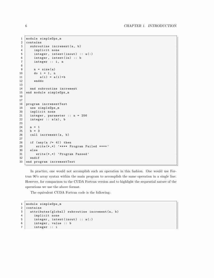
In practice, one would not accomplish such an operation in this fashion. One would use For-
tran 90’s array syntax within the main program to accomplish the same operation in a single line.
However, for comparison to the CUDA Fortran version and to highlight the sequential nature of the
operations we use the above format.
The equivalent CUDA Fortran code is the following:
1 module simpleOps_m
2 contains
3 attributes(global) subroutine increment(a, b)
4 implicit none
5 integer , intent(inout) :: a(:)
6 integer , value :: b
7 integer :: i
1.2. BASIC CONCEPTS 7
8
9 i = threadIdx%x
10 a(i) = a(i)+b
11
12 end subroutine increment
13 end module simpleOps_m
14
15
16 program incrementTest
17 use cudafor
18 use simpleOps_m
19 implicit none
20 integer , parameter :: n = 256
21 integer :: a(n), b
22 integer , device :: a_d(n)
23
24 a = 1
25 b = 3
26
27 a_d = a
28 call increment <<<1,n>>>(a_d , b)
29 a = a_d
30
31 if (any(a /= 4)) then
32 write (*,*) ’**** Program Failed ****’
33 else
34 write (*,*) ’Program Passed ’
35 endif
36 end program incrementTest
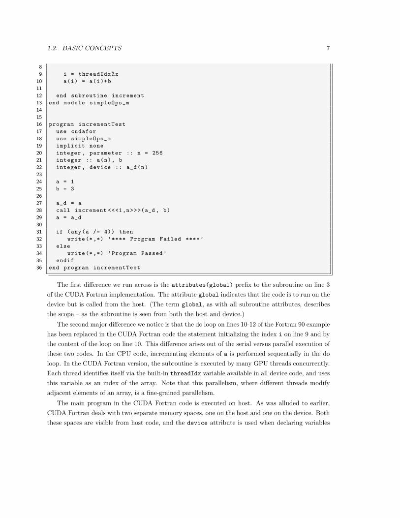
The first difference we run across is the attributes(global) prefix to the subroutine on line 3
of the CUDA Fortran implementation. The attribute global indicates that the code is to run on the
device but is called from the host. (The term global, as with all subroutine attributes, describes
the scope – as the subroutine is seen from both the host and device.)
The second major difference we notice is that the do loop on lines 10-12 of the Fortran 90 example
has been replaced in the CUDA Fortran code the statement initializing the index i on line 9 and by
the content of the loop on line 10. This difference arises out of the serial versus parallel execution of
these two codes. In the CPU code, incrementing elements of a is performed sequentially in the do
loop. In the CUDA Fortran version, the subroutine is executed by many GPU threads concurrently.
Each thread identifies itself via the built-in threadIdx variable available in all device code, and uses
this variable as an index of the array. Note that this parallelism, where different threads modify
adjacent elements of an array, is a fine-grained parallelism.
The main program in the CUDA Fortran code is executed on host. As was alluded to earlier,
CUDA Fortran deals with two separate memory spaces, one on the host and one on the device. Both
these spaces are visible from host code, and the device attribute is used when declaring variables
8 CHAPTER 1. INTRODUCTION
to indicate they reside in device memory, for example when declaring the device variable a d on
line 22 of the CUDA Fortran code. The “ d” suffix is not required but is a useful convention for
differentiating device from host variables in host code. Because CUDA Fortran is strongly typed
in this regard, data transfers between host and device can be performed by assignment statements.
This occurs on line 27, where after the array a is initialized on the host the data are transferred to
the device DRAM.
Once the data have been transferred to device DRAM, then the kernel, or subroutine that
executes on the device, can be launched as is done on line 28. The parameters specified in the triple
chevrons between the subroutine name and the argument list on line 28 are called the execution
configuration and determines the number of GPU threads used to execute the kernel. We will go
into the execution configuration in depth a bit later, but for now it is sufficient to say that an
execution configuration of <<<1,n>>> specifies that the kernel is executed by n GPU threads.
While kernel array arguments must reside in device memory, such as a d, this is not the case
with scalar arguments, such as the second kernel argument b. However, we need to make sure such
arguments are passed by value rather than by reference, since they reside in a different memory
space. Passing arguments by value is accomplished by using the value variable qualifier on line 6
of the CUDA Fortran code.
The data transfer from device to host on line 29 does not commence until the kernel has com-
pleted. This is a feature of data transfers and not the kernel execution. Once the kernel is launched,
control returns to the host immediately. However, the data transfer in line 29, or line 27 for that
matter, does not initiate until all previous operations on the GPU are complete and subsequent
operations on the GPU will not begin until the data transfer is complete. The blocking nature of
these data transfers are helpful in implicitly synchronizing the CPU and GPU. There are routines
that perform asynchronous transfers so that computation on the device can overlap communication
between host and device, as well as a means to synchronize host and device, which will be discussed
in Section 3.1.3
1.2.2 Extending to larger arrays
The above example has the limitation that with the execution configuration <<<1,n>>>, the pa-
rameter n and hence the array size must be small. This limit depends on the particular CUDA
device being used. On Fermi-based products, such at the Tesla C2050 card, the limit is n=1024,
and on previous generation cards this limit is n=512. The way to accommodate larger arrays is to
modify the first execution configuration parameter, as essentially the product of these two execution
configuration parameters gives the number of GPU threads that execute the code. So, why is this
done? Why are GPU threads grouped in this manner? This grouping of threads in the programming
model mimics the grouping of processing elements in hardware on the GPU.
1.2. BASIC CONCEPTS 9
Memory
GPUMultiprocessor
ThreadProcessors
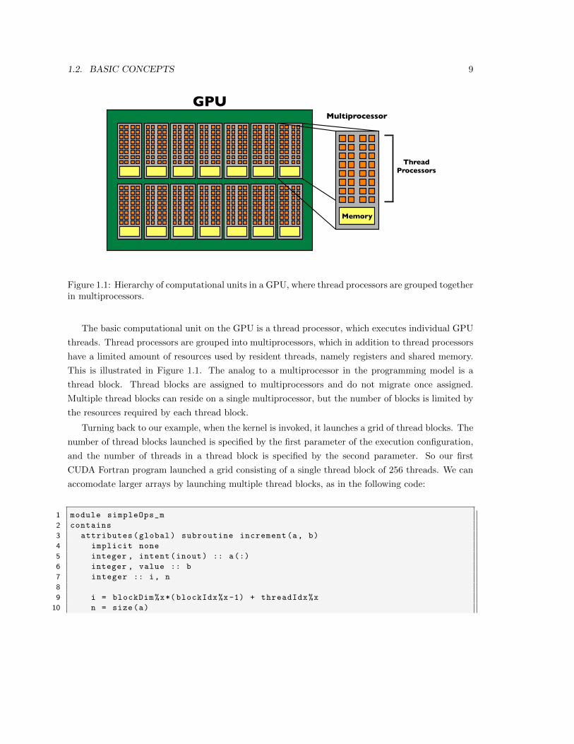
Figure 1.1: Hierarchy of computational units in a GPU, where thread processors are grouped togetherin multiprocessors.
The basic computational unit on the GPU is a thread processor, which executes individual GPU
threads. Thread processors are grouped into multiprocessors, which in addition to thread processors
have a limited amount of resources used by resident threads, namely registers and shared memory.
This is illustrated in Figure 1.1. The analog to a multiprocessor in the programming model is a
thread block. Thread blocks are assigned to multiprocessors and do not migrate once assigned.
Multiple thread blocks can reside on a single multiprocessor, but the number of blocks is limited by
the resources required by each thread block.
Turning back to our example, when the kernel is invoked, it launches a grid of thread blocks. The
number of thread blocks launched is specified by the first parameter of the execution configuration,
and the number of threads in a thread block is specified by the second parameter. So our first
CUDA Fortran program launched a grid consisting of a single thread block of 256 threads. We can
accomodate larger arrays by launching multiple thread blocks, as in the following code:
1 module simpleOps_m
2 contains
3 attributes(global) subroutine increment(a, b)
4 implicit none
5 integer , intent(inout) :: a(:)
6 integer , value :: b
7 integer :: i, n
8
9 i = blockDim%x*( blockIdx%x-1) + threadIdx%x
10 n = size(a)
10 CHAPTER 1. INTRODUCTION
11 if (i <= n) a(i) = a(i)+b
12
13 end subroutine increment
14 end module simpleOps_m
15
16
17 program incrementTest
18 use cudafor
19 use simpleOps_m
20 implicit none
21 integer , parameter :: n = 1024*1024
22 integer :: a(n), b
23 integer , device :: a_d(n)
24 integer :: tPB = 256
25
26 a = 1
27 b = 3
28
29 a_d = a
30 call increment <<<ceiling(real(n)/tPB),tPB >>>(a_d , b)
31 a = a_d
32
33 if (any(a /= 4)) then
34 write (*,*) ’**** Program Failed ****’
35 else
36 write (*,*) ’Program Passed ’
37 endif
38 end program incrementTest
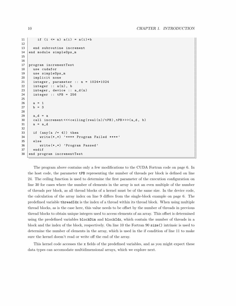
The program above contains only a few modifications to the CUDA Fortran code on page 6. In
the host code, the parameter tPB representing the number of threads per block is defined on line
24. The ceiling function is used to determine the first parameter of the execution configuration on
line 30 for cases where the number of elements in the array is not an even multiple of the number
of threads per block, as all thread blocks of a kernel must be of the same size. In the device code,
the calculation of the array index on line 9 differs from the single-block example on page 6. The
predefined variable threadIdx is the index of a thread within its thread block. When using multiple
thread blocks, as is the case here, this value needs to be offset by the number of threads in previous
thread blocks to obtain unique integers used to access elements of an array. This offset is determined
using the predefined variables blockDim and blockIdx, which contain the number of threads in a
block and the index of the block, respectively. On line 10 the Fortran 90 size() intrinsic is used to
determine the number of elements in the array, which is used in the if condition of line 11 to make
sure the kernel doesn’t read or write off the end of the array.
This kernel code accesses the x fields of the predefined variables, and as you might expect these
data types can accomodate multidimensional arrays, which we explore next.
1.2. BASIC CONCEPTS 11
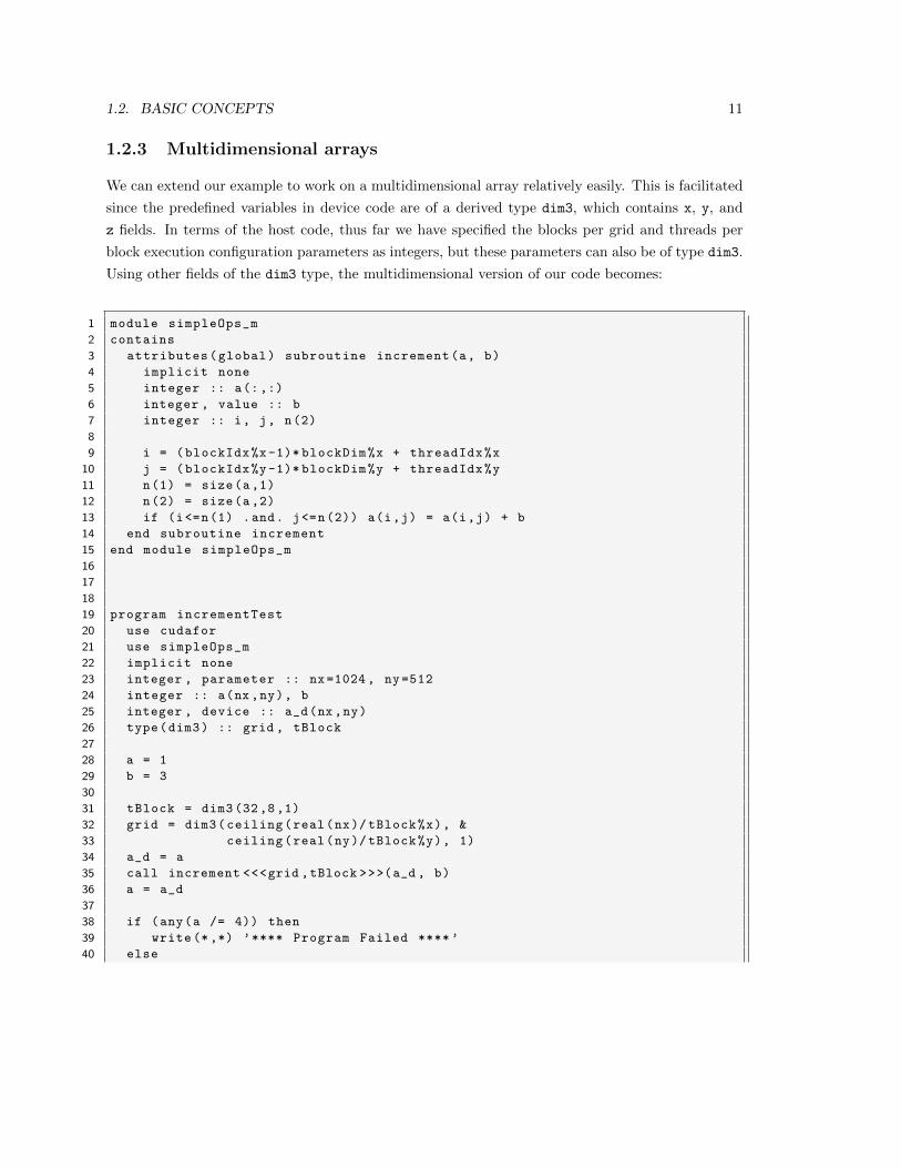
1.2.3 Multidimensional arrays
We can extend our example to work on a multidimensional array relatively easily. This is facilitated
since the predefined variables in device code are of a derived type dim3, which contains x, y, and
z fields. In terms of the host code, thus far we have specified the blocks per grid and threads per
block execution configuration parameters as integers, but these parameters can also be of type dim3.
Using other fields of the dim3 type, the multidimensional version of our code becomes:
1 module simpleOps_m
2 contains
3 attributes(global) subroutine increment(a, b)
4 implicit none
5 integer :: a(:,:)
6 integer , value :: b
7 integer :: i, j, n(2)
8
9 i = (blockIdx%x-1)* blockDim%x + threadIdx%x
10 j = (blockIdx%y-1)* blockDim%y + threadIdx%y
11 n(1) = size(a,1)
12 n(2) = size(a,2)
13 if (i<=n(1) .and. j<=n(2)) a(i,j) = a(i,j) + b
14 end subroutine increment
15 end module simpleOps_m
16
17
18
19 program incrementTest
20 use cudafor
21 use simpleOps_m
22 implicit none
23 integer , parameter :: nx=1024 , ny=512
24 integer :: a(nx ,ny), b
25 integer , device :: a_d(nx ,ny)
26 type(dim3) :: grid , tBlock
27
28 a = 1
29 b = 3
30
31 tBlock = dim3 (32,8,1)
32 grid = dim3(ceiling(real(nx)/ tBlock%x), &
33 ceiling(real(ny)/ tBlock%y), 1)
34 a_d = a
35 call increment <<<grid ,tBlock >>>(a_d , b)
36 a = a_d
37
38 if (any(a /= 4)) then
39 write (*,*) ’**** Program Failed ****’
40 else
12 CHAPTER 1. INTRODUCTION
41 write (*,*) ’Program Passed ’
42 endif
43 end program incrementTest
After declaring the parameters nx and ny along with the host and device arrays for this two-
dimensional example, we declare two variables of type dim3 used in the execution configuration on
line 26. On line 31 the three components of the dim3 type specifying the number of threads per
block are set, in the case each block has a 32× 8 arrangement of threads. In the following two lines,
the ceiling function is used to determine the number of blocks in the x and y dimensions required
to increment all the elements of the array. The kernel is then launched with these variables as the
execution configuration parameters in line 35. In the kernel code, the dummy argument a is declared
as a two-dimensional array and the variable n as a two-element array which on lines 11 and 12 is
set to hold the size of a in each dimension. An additional index j is set on line 10 in an analogous
manner to i, and both i and j are checked for in-bounds access before a(i,j) is incremented.
1.3 Determining CUDA Hardware Features and Limits
There are many different CUDA-capable cards available, spanning different product lines (GeForce
and Quadro as well as Tesla) in addition to different architecture versions. We have already discussed
the limitation of the number of threads per block, which is 1024 on Fermi-based hardware and 512
for previous architecture generations, and there are many other features and limitations that very
between different cards. In this section we cover the device management API which contains routines
for determining the number and what types of CUDA-capable cards are available on a particular
system and what features and limits such cards have.
Before we go into the device management API, we should briefly discuss the notion of compute
capability. The compute capability of CUDA-enabled cards reflects the generation of the architecture
and is given in Major.Minor format. The very first CUDA-enabled cards were of compute capability
1.0. Fermi-generation cards have a compute capability of 2.x. Some features of CUDA correlate with
the compute capability, for example double precision is available with cards of compute capability
1.3 and higher. Other features do not correlate with compute capability, but can be determined
through the device management API.
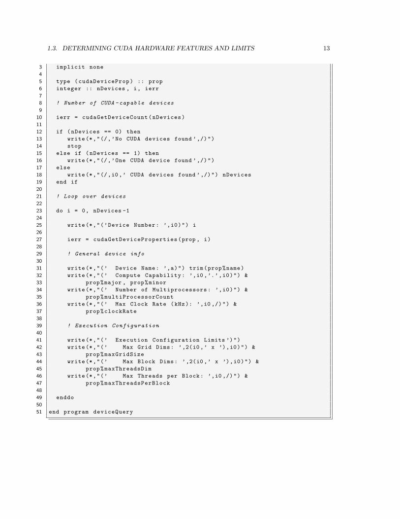
The device management API has routines for getting information on the number of cards avail-
able on a system, as well as for selecting a card amongst available cards. This API makes use
of the cudaDeviceProp derived type for inquiring about the features of individual cards, which is
demonstrated in the program below.
1 program deviceQuery
2 use cudafor
1.3. DETERMINING CUDA HARDWARE FEATURES AND LIMITS 13
3 implicit none
4
5 type (cudaDeviceProp) :: prop
6 integer :: nDevices , i, ierr
7
8 ! Number of CUDA -capable devices
9
10 ierr = cudaGetDeviceCount(nDevices)
11
12 if (nDevices == 0) then
13 write(*,"(/,’No CUDA devices found ’,/)")
14 stop
15 else if (nDevices == 1) then
16 write(*,"(/,’One CUDA device found ’,/)")
17 else
18 write(*,"(/,i0 ,’ CUDA devices found ’,/)") nDevices
19 end if
20
21 ! Loop over devices
22
23 do i = 0, nDevices -1
24
25 write(*,"(’Device Number: ’,i0)") i
26
27 ierr = cudaGetDeviceProperties(prop , i)
28
29 ! General device info
30
31 write(*,"(’ Device Name: ’,a)") trim(prop%name)
32 write(*,"(’ Compute Capability: ’,i0 ,’.’,i0)") &
33 prop%major , prop%minor
34 write(*,"(’ Number of Multiprocessors: ’,i0)") &
35 prop%multiProcessorCount
36 write(*,"(’ Max Clock Rate (kHz): ’,i0 ,/)") &
37 prop%clockRate
38
39 ! Execution Configuration
40
41 write(*,"(’ Execution Configuration Limits ’)")
42 write(*,"(’ Max Grid Dims: ’,2(i0 ,’ x ’),i0)") &
43 prop%maxGridSize
44 write(*,"(’ Max Block Dims: ’,2(i0 ,’ x ’),i0)") &
45 prop%maxThreadsDim
46 write(*,"(’ Max Threads per Block: ’,i0 ,/)") &
47 prop%maxThreadsPerBlock
48
49 enddo
50
51 end program deviceQuery
14 CHAPTER 1. INTRODUCTION
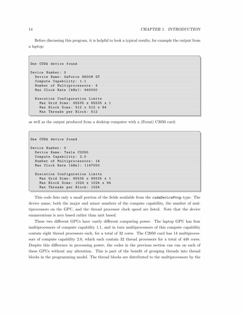
Before discussing this program, it is helpful to look a typical results, for example the output from
a laptop:
� �One CUDA device found
Device Number: 0
Device Name: GeForce 8600M GT
Compute Capability: 1.1
Number of Multiprocessors: 4
Max Clock Rate (kHz): 940000
Execution Configuration Limits
Max Grid Dims: 65535 x 65535 x 1
Max Block Dims: 512 x 512 x 64
Max Threads per Block: 512�as well as the output produced from a desktop computer with a (Fermi) C2050 card:
� �One CUDA device found
Device Number: 0
Device Name: Tesla C2050
Compute Capability: 2.0
Number of Multiprocessors: 14
Max Clock Rate (kHz): 1147000
Execution Configuration Limits
Max Grid Dims: 65535 x 65535 x 1
Max Block Dims: 1024 x 1024 x 64
Max Threads per Block: 1024�This code lists only a small portion of the fields available from the cudaDeviceProp type. The
device name, both the major and minor numbers of the compute capability, the number of mul-
tiprocessors on the GPU, and the thread processor clock speed are listed. Note that the device
enumerations is zero based rather than unit based.
These two different GPUs have vastly different computing power. The laptop GPU has four
multiprocessors of compute capability 1.1, and in turn multiprocessors of this compute capability
contain eight thread processors each, for a total of 32 cores. The C2050 card has 14 multiproces-
sors of compute capability 2.0, which each contain 32 thread processors for a total of 448 cores.
Despite this difference in processing power, the codes in the previous section can run on each of
these GPUs without any alteration. This is part of the benefit of grouping threads into thread
blocks in the programming model. The thread blocks are distributed to the multiprocessors by the
1.3. DETERMINING CUDA HARDWARE FEATURES AND LIMITS 15
scheduler as space becomes available. Thread blocks are independent, so the order in which they
execute does not affect the outcome. This independence of thread blocks in the programming model
allows the scheduling to be done behind the scenes, so that the programmer need only worry about
programming for threads within a thread block.
In addition to these hardware characteristics, the deviceQuery code also lists limits of the
execution configuration for the two devices. The only difference here is the maximum number
threads per block, which we alluded to earlier, as well as how these threads can be arranged within
the thread block. Of note here is that the grid of thread blocks launched by a kernel can be quite
large and is the same for both cards – one can launch a kernel with over 1012 threads on either
device! Once again the independence of thread blocks allows the scheduler to assign thread blocks
to multiprocessors as space becomes available, all of which is done without intervention by the
programmer.
The pgaccelinfo utility included with the PGI compilers provides the information presented in
deviceQuery and more.
1.3.1 Single and double precision
One of the features that is determined by the compute capability is whether or not double precision
floating point types are supported. For the Tesla product line, devices of compute capability 1.3
and higher (eg. C1060 and C2050) support double precision variables. While large applications will
be deployed on systems with these GPUs, it is often convenient to develop code on systems which
do not support doubles (eg. laptops).
Luckily, Fortran 90’s kind type parameters allows us to accomodate switching between single
and double precision quite easily. All one had to do is to define a module with the selected kind:
module precision_m
integer , parameter :: singlePrecision = kind (0.0)
integer , parameter :: doublePrecision = kind (0.0d0)
! Comment out one of the lines below
integer , parameter :: fp_kind = singlePrecision
!integer , parameter :: fp_kind = doublePrecision
end module precision_m
and then use this module and the parameter fp kind when declaring floating point variables in code:
use precision_m
real(fp_kind), device :: a_d(n)
16 CHAPTER 1. INTRODUCTION
This allows one to toggle between the two precisions simply by changing the fp kind definition in
the precision module. (One may have to write some generic interfaces to accomodate library calls
such as CUFFT routines.)
Another option for toggling between single and double precision that doesn’t involve modifying
source code is through use of the preprocessor, where the precision module can be modified as:
module precision_m
integer , parameter :: singlePrecision = kind (0.0)
integer , parameter :: doublePrecision = kind (0.0d0)
#ifdef DOUBLE
integer , parameter :: fp_kind = doublePrecision
#else
integer , parameter :: fp_kind = singlePrecision
#endif
end module precision_m
Here one can compile for double precision by compiling the precision module with the compiler
options -Mpreprocess -DDOUBLE.
We make extensive use of the precision module throughout this document for several reasons.
The first is that it allows the reader to use the example codes on whatever card they have available.
It allows us to easily assess the performance characteristics of the two precisions on various codes.
And finally, it is a good practice in terms of code reuse.
This technique can be extended to facilitate mixed-precision code. For example, in a code
simulating reacting flow one may want to experiment with different precisions for the flow variables
and chemical species. To do so one can declare variables in the code as follows:
real(flow_kind), device :: u(nx,ny,nz), v(nx,ny,nz), w(nx,ny,nz)
real(chemistry_kind), device :: q(nx,ny,nz,nspecies)
where flow kind and chemistry kind are declared as either single or double precision in the
precision m module.
1.4 Error Handling
The return values for the host CUDA functions in the device query example, as well as all host CUDA
API functions, can be used check for errors that occurred during their execution. To illustrate such
error handling, the successful execution of cudaGetDeviceCount() of line 10 in the deviceQuery
example can be checked as follows:
1.5. COMPILING CUDA FORTRAN CODE 17
ierr = cudaGetDeviceCount(nDevices)
if (ierr /= cudaSuccess) write (*,*) cudaGetErrorString(ierr)
The variable cudaSuccess is defined in the cudafor module that is used in this code. If there is an
error, then the function cudaGetErrorString() is used to return a character string describing the
error, as opposed to just listing the numeric error code.
Error handling of kernels is a bit more complicated since kernels are subroutines and there-
fore do not have a return value. For kernels, some errors will be caught by CUDA Fortran, such
as when an execution configuration is specified that exceeds hardware limits. However, because
the kernel is executed asynchronously, errors may occur on the device after control is returned
to the host, so the cudaThreadSynchronize()1 or some other synchronization call is required.
cudaThreadSynchronize() blocks the host thread until all previously issued commands, such as
the kernel launch, have completed. Successful completion of kernels can be checked as shown in the
modified increment code below:
call increment <<<1,n>>>(a_d , b)
ierr = cudaThreadSynchronize ()
if (ierr /= cudaSuccess) write (*,*) cudaGetErrorString(ierr)
Any error that occurs on the device after control is returned to the GPU will be reflected in the
return value of cudaThreadSynchronize(). Another command that is useful for checking errors is
cudaGetLastError(), which returns the error code of the last device operation – such as device mem-
ory allocation, data transfer, or kernel) – on the GPU. One should note that cudaGetLastError()
resets the error flag, so it can not be used twice to recover the same error.
1.5 Compiling CUDA Fortran Code
CUDA Fortran codes are compiled using PGI Fortran compiler. Files with the .cuf or .CUF exten-
sions have CUDA Fortran enabled automatically, and the compiler option -Mcuda can be used when
compiling file with other extensions to enable CUDA Fortran. Compilation of CUDA Fortran code
can be as simple as issuing the command:� �pgf90 increment.cuf�
Behind the scenes, a multistep process takes place. The first step is a source-to-source compilation
where CUDA C device code is generated by CUDA Fortran. From here compilation is similar to
1In CUDA 4.0 the routine cudaDeviceSynchronize() is preferred to cudaThreadSynchronize() as the former is amore accurate in the context of the multi-GPU features introduced in that version. However, we use the latter forbackwards compatibility throughout this book.
18 CHAPTER 1. INTRODUCTION
compilation of CUDA C. The device code is compiled into a intermediate representation called PTX
(Parallel Thread eXecution), which is a format common to all CUDA capable devices. The PTX
code is then further compiled to a executable code for a particular compute capability. The host
code is compiled using the native host compiler. The final executable contains the host binary, the
device binary, and the PTX. The PTX is included so that a new device binary can be created when
the executable is run on a card of different compute capability than originally compiled for.
Specifics of the above compilation process can be controlled through options to -Mcuda. A
specific compute capability can be targeted, for example -Mcuda=cc20 generates executables for
devices of compute capability 2.0. There is an emulation mode where device code is run on the
host, specified by -Mcuda=emu. Also, double precision is only available when compiling for compute
capability 1.3 and higher. CUDA Fortran can use several versions of the CUDA Toolkit, for example
-Mcuda=cuda3.1.
CUDA has a set of fast, but less accurate, intrinsics for single precision functions like sin()
and cos() which can be enabled by -Mcuda=fastmath. The option -Mucda=maxregcount:N can by
used to limit the number of registers used per thread to N. And the option -Mcuda=ptxinfo prints
information on memory usage in kernels.
To see all of the options available through the compiler type pgf90 -help on the command line.
1.6 System and Environment Management
In addition to compiler flags, there are a variety of environment variables that can control certain
aspects of CUDA Fortran execution:
CUDA LAUNCH BLOCKING when set to 1 forces execution of kernels to be synchronous. That is, after
launching a kernel control will return to the CPU only after the kernel has completed. This
provides an efficient way to check whether host-device synchronization errors are responsible
for unexpected behavior. By default the value is 0.
COMPUTE PROFILE, COMPUTE PROFILE CONFIG are used to control profiling, these will be discussed
in detail in Section 2.1.3. By default profiling is turned off.
CUDA VISIBLE DEVICES can be used to make certain devices invisible on the system, and to change
the enumeration of devices. A comma separated list of integers is assigned to this variable which
contains the visible devices and their enumeration as seen from the subsequent execution of
CUDA Fortran programs. (One can use the deviceQuery code presented earlier, or the utility
pgaccelinfo to obtain the default enumeration of devices.)
Additional control of devices on a system is available through the nvidia-smi, the System
Management Interface utility available on Linux platforms. This utility can give information on all

1.6. SYSTEM AND ENVIRONMENT MANAGEMENT 19
GPUs on the system (whether CUDA capable or not), report the current ECC settings as well as
toggle them on or off (which required a reboot), and set the compute modes for the GPU (normal
mode, exclusive mode where only one compute context can access a GPU, or prohibited mode where
the GPU is not available for computation). Refer to the man pages for nvidia-smi for a complete
description of this utility.

20 CHAPTER 1. INTRODUCTION
Chapter 2
Performance Measurement and
Metrics
A prerequisite to performance optimization is a means to accurately time portions of a code, and
subsequently how to use such timing information to assess code performance. In this chapter we first
discuss how to time kernel execution using CPU timers, CUDA events, and the CUDA Profiler. We
then discuss how timing information can be used to determine the limiting factor of kernel execution.
Finally, we discuss how to calculate performance metrics, especially related to bandwidth, and how
such metrics should be interpreted.
2.1 Measuring Kernel Execution Time
There are several ways to measure kernel execution time. One can use traditional CPU timers, but
in doing so one must be careful to ensure correct synchronization between host and device for such
measurement to be accurate. The CUDA event API routines which are called from host code can be
used to calculate kernel execution time using the device clock. Finally, we discuss how the CUDA
Profiler can be used from the command-line to give this timing information.
2.1.1 Host-device synchronization and CPU timers
Care must be taken when timing GPU routines using traditional CPU timers. From the host
perspective, kernel execution as well as many CUDA Fortran API functions are nonblocking or
asynchronous: they return control back to the calling CPU thread prior to completing their work.
For example, in the following code segment:
21
22 CHAPTER 2. PERFORMANCE MEASUREMENT AND METRICS
a_d = a
call increment <<<1,n>>>(a_d , b)
a = a_d
once the increment kernel is launched in line 2 control returns to the CPU. By contrast, the data
transfers before and after the kernel launch are synchronous or blocking. Such data transfers do not
begin until all previously issued CUDA calls have completed, and subsequent CUDA calls will not
begin until the transfer has completed.1 Given the synchronous nature of the data transfers, the
above code section executes safely: the kernel call isn’t launched until the previously issued data
transfer completes, and the following data transfer doesn’t commence until the kernel has completed.
However, if we modify the code to time kernel execution we need to be explicitly synchronize the
CPU thread using cudaThreadSynchronize()2:
1 a_d = a
2 t1 = myCPUTimer ()
3 call increment <<<1,n>>>(a_d , b)
4 istat = cudaThreadSynchronize ()
5 t2 = myCPUTimer ()
6 a = a_d
The function cudaThreadSynchronize() blocks the calling CPU thread until all CUDA calls previ-
ously issued by the thread are completed, which is required for correct measurement of increment. It
is a best practice is to call cudaThreadSynchronize() before any timing call. For example, inserting
a cudaThreadSynchronize() before line 2 would be well advised even though not required as one
might change the transfer at line 1 to an asynchronous transfer and forget to add the synchronization
call.
An alternative to using the function cudaThreadSynchronize() is to set the environment vari-
able CUDA LAUNCH BLOCKING to 1, which turns kernel invocations into synchronous function calls.
However, this would apply to all kernel launches of a program, and would therefore serialize any
CPU code with kernel execution.
2.1.2 Timing via CUDA events
One problem with host-device synchronization points, such as those produced by the function
cudaThreadSynchronize() and the environment variable CUDA LAUNCH BLOCKING, is that they stall
the GPU’s processing pipeline. Unfortunately, such synchronization points are required using CPU
timers. Luckily, CUDA offers a relatively light-weight alternative to using CPU timers via the CUDA
1Note that asynchronous versions of data transfers are available using the cudaMemcpy*Async() routines which willbe discussed in Section 3.1.3.
2When using the CUDA 4.0 toolkit and above cudaDeviceSynchronize() is the preferred routine name for syn-chronization due to those versions’ multi-GPU capabilities, although cudaThreadSynchronize() is still recognized.
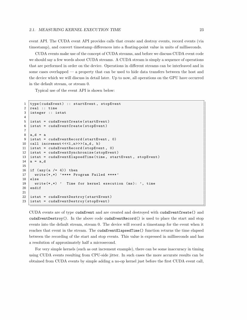
2.1. MEASURING KERNEL EXECUTION TIME 23
event API. The CUDA event API provides calls that create and destroy events, record events (via
timestamp), and convert timestamp differences into a floating-point value in units of milliseconds.
CUDA events make use of the concept of CUDA streams, and before we discuss CUDA event code
we should say a few words about CUDA streams. A CUDA stream is simply a sequence of operations
that are performed in order on the device. Operations in different streams can be interleaved and in
some cases overlapped — a property that can be used to hide data transfers between the host and
the device which we will discuss in detail later. Up to now, all operations on the GPU have occurred
in the default stream, or stream 0.
Typical use of the event API is shown below:
1 type(cudaEvent) :: startEvent , stopEvent
2 real :: time
3 integer :: istat
4
5 istat = cudaEventCreate(startEvent)
6 istat = cudaEventCreate(stopEvent)
7
8 a_d = a
9 istat = cudaEventRecord(startEvent , 0)
10 call increment <<<1,n>>>(a_d , b)
11 istat = cudaEventRecord(stopEvent , 0)
12 istat = cudaEventSynchronize(stopEvent)
13 istat = cudaEventElapsedTime(time , startEvent , stopEvent)
14 a = a_d
15
16 if (any(a /= 4)) then
17 write (*,*) ’**** Program Failed ****’
18 else
19 write (*,*) ’ Time for kernel execution (ms): ’, time
20 endif
21
22 istat = cudaEventDestroy(startEvent)
23 istat = cudaEventDestroy(stopEvent)
CUDA events are of type cudaEvent and are created and destroyed with cudaEventCreate() and
cudaEventDestroy(). In the above code cudaEventRecord() is used to place the start and stop
events into the default stream, stream 0. The device will record a timestamp for the event when it
reaches that event in the stream. The cudaEventElapsedTime() function returns the time elapsed
between the recording of the start and stop events. This value is expressed in milliseconds and has
a resolution of approximately half a microsecond.
For very simple kernels (such as out increment example), there can be some inaccuracy in timing
using CUDA events resulting from CPU-side jitter. In such cases the more accurate results can be
obtained from CUDA events by simple adding a no-op kernel just before the first CUDA event call,
24 CHAPTER 2. PERFORMANCE MEASUREMENT AND METRICS
so that the cudaEventRecord() and subsequent kernel call will be queued up on the GPU.
2.1.3 Command-line profiler
Timing information can also be obtained from the CUDA profiler, which can be used from the
command line. This approach does not require instrumentation of code as needed in the case with
CUDA events. It doesn’t even require recompilation of the source code with special flags. Profiling
can be enabled by setting the environment variable COMPUTE PROFILE to 1, as is done when profiling
in CUDA C code.
The environment variable COMPUTE PROFILE CONFIG specifies the file containing a list of perfor-
mance counters to use. A list of the counters for various CUDA architectures, as well as their inter-
pretation, is given in the profiler documentation provided with the CUDA Toolkit, which can be ob-
tained online. Discussion of the counters used in this document is deferred until the relevant sections
of the Chapter 3. However, it should be noted that profiling certain counters causes operations on
the GPU to be serialized, so that asynchronous data transfers using multiple streams is not possible
when accessing such counters. Without specifying a configuration file via COMPUTE PROFILE CONFIG,
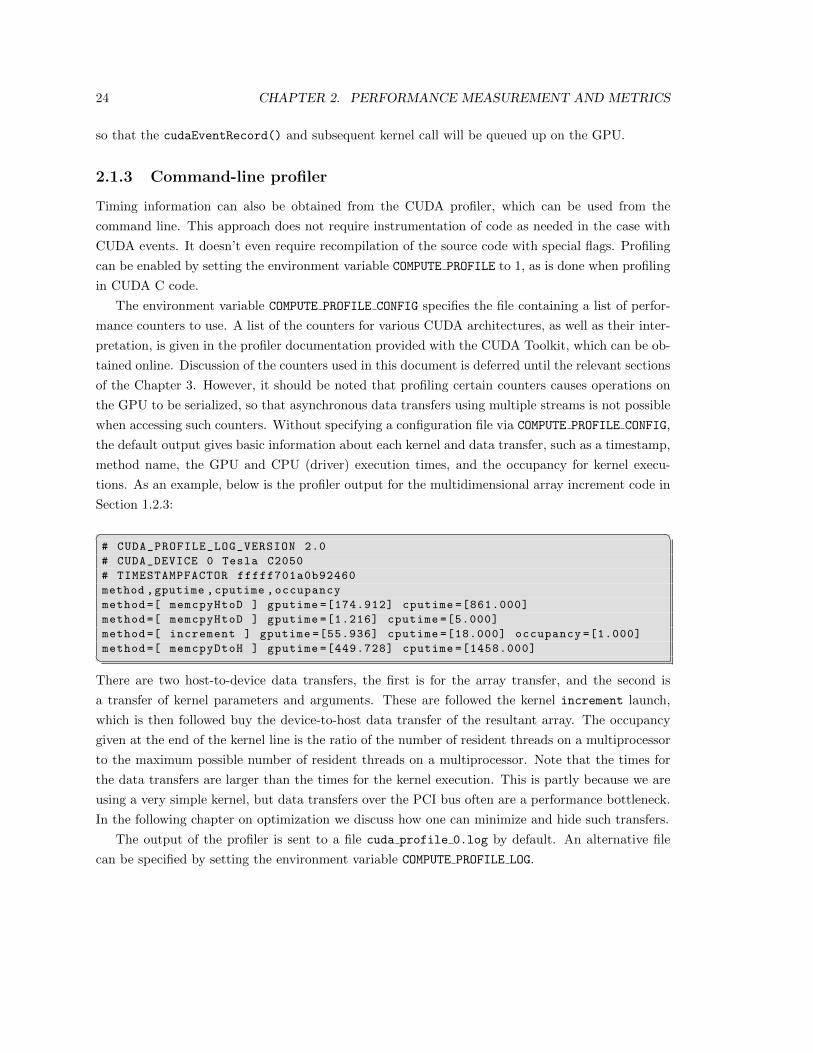
the default output gives basic information about each kernel and data transfer, such as a timestamp,
method name, the GPU and CPU (driver) execution times, and the occupancy for kernel execu-
tions. As an example, below is the profiler output for the multidimensional array increment code in
Section 1.2.3:� �# CUDA_PROFILE_LOG_VERSION 2.0
# CUDA_DEVICE 0 Tesla C2050
# TIMESTAMPFACTOR fffff701a0b92460
method ,gputime ,cputime ,occupancy
method =[ memcpyHtoD ] gputime =[174.912] cputime =[861.000]
method =[ memcpyHtoD ] gputime =[1.216] cputime =[5.000]
method =[ increment ] gputime =[55.936] cputime =[18.000] occupancy =[1.000]
method =[ memcpyDtoH ] gputime =[449.728] cputime =[1458.000]�There are two host-to-device data transfers, the first is for the array transfer, and the second is
a transfer of kernel parameters and arguments. These are followed the kernel increment launch,
which is then followed buy the device-to-host data transfer of the resultant array. The occupancy
given at the end of the kernel line is the ratio of the number of resident threads on a multiprocessor
to the maximum possible number of resident threads on a multiprocessor. Note that the times for
the data transfers are larger than the times for the kernel execution. This is partly because we are
using a very simple kernel, but data transfers over the PCI bus often are a performance bottleneck.
In the following chapter on optimization we discuss how one can minimize and hide such transfers.
The output of the profiler is sent to a file cuda profile 0.log by default. An alternative file
can be specified by setting the environment variable COMPUTE PROFILE LOG.
2.2. INSTRUCTION, BANDWIDTH, AND LATENCY BOUND KERNELS 25
2.2 Instruction, Bandwidth, and Latency Bound Kernels
Having the ability to time kernel execution, we can now talk about how to determine what is the
limiting factor of a kernel’s execution. There are several ways to do this. One option is to use of the
profiler’s hardware counters, but the counters used for such an analysis likely change from generation
to generation of hardware. Instead, we describe in this section a method that is more general in
that the same procedure will work regardless of the generation of the hardware. In fact this method
can be applied to CPU platforms as well as GPUs. For this method, multiple versions of the kernel
are created which expose the memory and math intensive aspects of the full kernel. Each kernel
is timed, and a comparison of these times can reveal the limiting factor of kernel execution. This
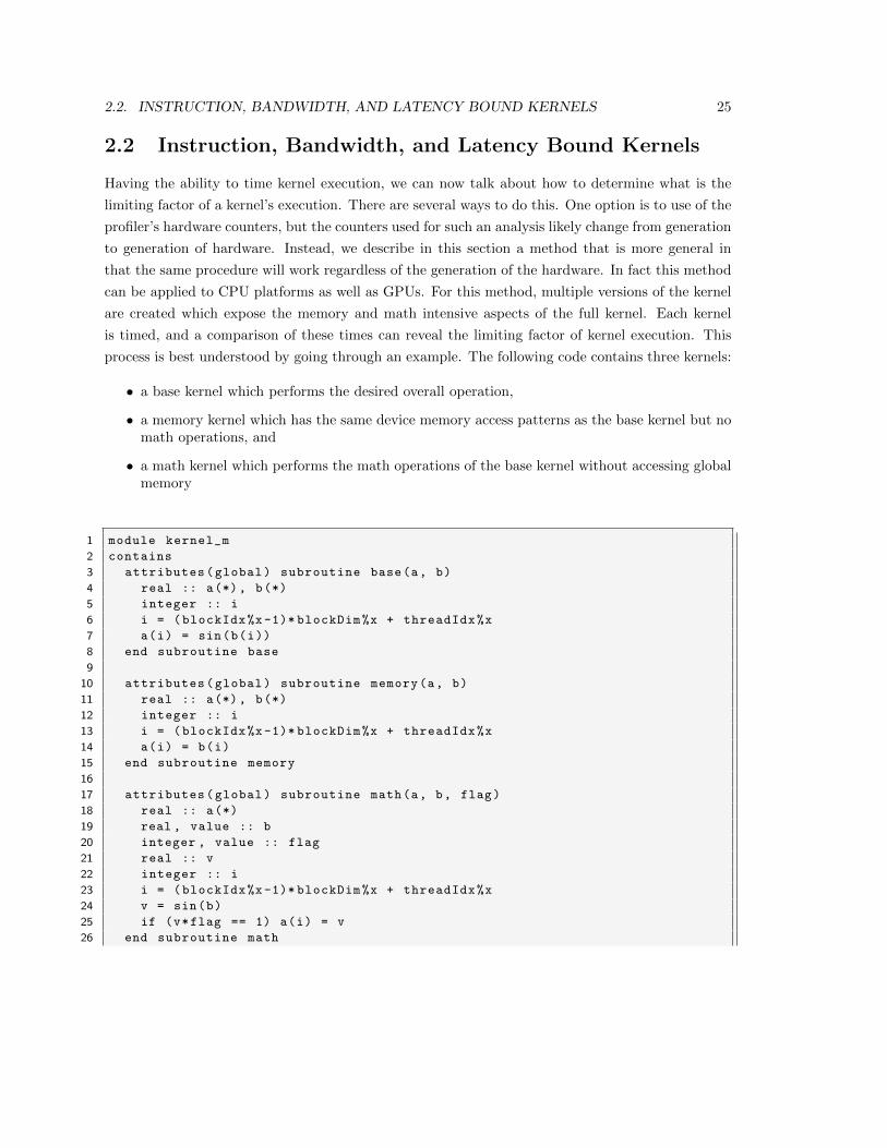
process is best understood by going through an example. The following code contains three kernels:
• a base kernel which performs the desired overall operation,
• a memory kernel which has the same device memory access patterns as the base kernel but nomath operations, and
• a math kernel which performs the math operations of the base kernel without accessing globalmemory
1 module kernel_m
2 contains
3 attributes(global) subroutine base(a, b)
4 real :: a(*), b(*)
5 integer :: i
6 i = (blockIdx%x-1)* blockDim%x + threadIdx%x
7 a(i) = sin(b(i))
8 end subroutine base
9
10 attributes(global) subroutine memory(a, b)
11 real :: a(*), b(*)
12 integer :: i
13 i = (blockIdx%x-1)* blockDim%x + threadIdx%x
14 a(i) = b(i)
15 end subroutine memory
16
17 attributes(global) subroutine math(a, b, flag)
18 real :: a(*)
19 real , value :: b
20 integer , value :: flag
21 real :: v
22 integer :: i
23 i = (blockIdx%x-1)* blockDim%x + threadIdx%x
24 v = sin(b)
25 if (v*flag == 1) a(i) = v
26 end subroutine math
26 CHAPTER 2. PERFORMANCE MEASUREMENT AND METRICS
27 end module kernel_m
28
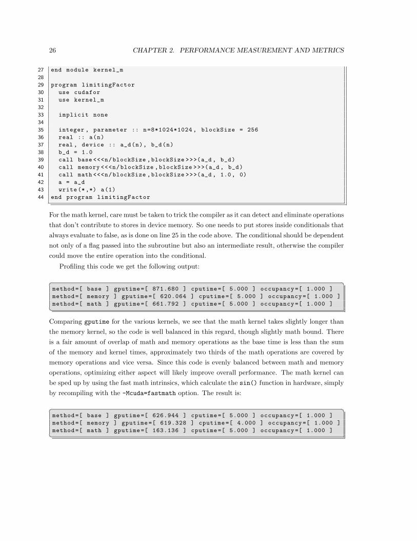
29 program limitingFactor
30 use cudafor
31 use kernel_m
32
33 implicit none
34
35 integer , parameter :: n=8*1024*1024 , blockSize = 256
36 real :: a(n)
37 real , device :: a_d(n), b_d(n)
38 b_d = 1.0
39 call base <<<n/blockSize ,blockSize >>>(a_d , b_d)
40 call memory <<<n/blockSize ,blockSize >>>(a_d , b_d)
41 call math <<<n/blockSize ,blockSize >>>(a_d , 1.0, 0)
42 a = a_d
43 write (*,*) a(1)
44 end program limitingFactor
For the math kernel, care must be taken to trick the compiler as it can detect and eliminate operations
that don’t contribute to stores in device memory. So one needs to put stores inside conditionals that
always evaluate to false, as is done on line 25 in the code above. The conditional should be dependent
not only of a flag passed into the subroutine but also an intermediate result, otherwise the compiler
could move the entire operation into the conditional.
Profiling this code we get the following output:
� �method =[ base ] gputime =[ 871.680 ] cputime =[ 5.000 ] occupancy =[ 1.000 ]
method =[ memory ] gputime =[ 620.064 ] cputime =[ 5.000 ] occupancy =[ 1.000 ]
method =[ math ] gputime =[ 661.792 ] cputime =[ 5.000 ] occupancy =[ 1.000 ]�Comparing gputime for the various kernels, we see that the math kernel takes slightly longer than
the memory kernel, so the code is well balanced in this regard, though slightly math bound. There
is a fair amount of overlap of math and memory operations as the base time is less than the sum
of the memory and kernel times, approximately two thirds of the math operations are covered by
memory operations and vice versa. Since this code is evenly balanced between math and memory
operations, optimizing either aspect will likely improve overall performance. The math kernel can
be sped up by using the fast math intrinsics, which calculate the sin() function in hardware, simply
by recompiling with the -Mcuda=fastmath option. The result is:
� �method =[ base ] gputime =[ 626.944 ] cputime =[ 5.000 ] occupancy =[ 1.000 ]
method =[ memory ] gputime =[ 619.328 ] cputime =[ 4.000 ] occupancy =[ 1.000 ]
method =[ math ] gputime =[ 163.136 ] cputime =[ 5.000 ] occupancy =[ 1.000 ]�
2.3. MEMORY BANDWIDTH 27
As expected, the time for the math kernel goes down considerably, and along with it the base kernel
time. The base kernel is now memory bound, as the memory and base kernels run in almost the
same amount of time: the math operations are nearly entirely hidden my memory operations. At
this point further improvement can only come from optimizing device memory accesses, if possible.
Deciding whether or not one can improve memory accesses motivates the next section on memory
bandwidth. But before we jump into bandwidth metrics, we need to tie up some loose ends regarding
this technique of modifying source code to determine the limiting factor of a kernel.
When there is very little overlap of math and memory operations, a kernel is likely latency bound.
This often occurs when the occupancy is low, there simply are not enough threads on the device
at one time for any overlap of operations. The remedy for this can often be a modification to the
execution configuration.
The reason for using the profiler for time measurement in this analysis is twofold. The first is that
it requires no instrumentation of the host code. (We have already written two additional kernels, so
this is welcome.) The second is that we want to make sure that the occupancy is the same for all our
kernels. When we remove math operations from a kernel, we likely reduce the number of registers
used (which can be checked using the -Mcuda=ptxinfo flag). If the register usage varies enough,
the occupancy, or fraction of actual to maximum number of threads resident on a multiprocessor,
can change which will affect run times. In our example the occupancy is everywhere 1.0, but if this
is not the case then one can lower the occupancy by allocating shared memory in the kernel via a
third argument to the execution configuration. This optional argument is the number of bytes of
dynamically allocated shared memory that is used for each thread block. We will talk more about
shared memory in Section 3.3.3, but for now all we need to know is that shared memory can be
reserved for a thread block simply by providing the number of bytes per thread block as a third
argument to the execution configuration.
2.3 Memory Bandwidth
Returning to the example code in Section 2.2, we are left with a memory bound kernel after using
the fast math intrinsics to reduce time spent on evaluation of sin(). At this stage we ask how well
is the memory system used, and whether there is room for improvement. To answer this question,
we need to calculate the memory bandwidth.
Bandwidth — the rate at which data can be transferred — is one of the most important gating
factors for performance. Almost all changes to code should be made in the context of how they
affect bandwidth. Bandwidth can be dramatically affected by the choice of memory in which data
is stored, how the data is laid out and the order in which it is accessed, as well as other factors.
When evaluating bandwidth, both the theoretical peak bandwidth and the observed or effective
memory bandwidth are used. When the latter is much lower than the former, design or imple-
28 CHAPTER 2. PERFORMANCE MEASUREMENT AND METRICS
mentation details are likely to reduce bandwidth, and it should be the primary goal of subsequent
optimization efforts to increase it.
2.3.1 Theoretical bandwidth
Theoretical bandwidth can be calculated using hardware specifications available in the product
literature. For example, the NVIDIA Tesla C2050 uses DDR (double data rate) RAM with a
memory clock rate of 1,500 MHz and a 384-bit wide memory interface. Using these data items, the
peak theoretical memory bandwidth of the NVIDIA Tesla C2050 is 144 GB/sec:
BWTheoretical =1500× 106 × (384/8)× 2
109= 144 GBps
In this calculation, the memory clock rate is converted in to Hz, multiplied by the interface width
(divided by 8, to convert bits to bytes) and multiplied by 2 due to the double data rate. Finally,
this product is divided by 109 to convert the result to GB/sec (GBps).3
For devices with ECC, one also needs to consider the effect of ECC on peak bandwidth. As a
rough rule of thumb, one would expect the theoretical bandwidth on a device with ECC enabled to
be 85% of the bandwidth without ECC. So for the C2050 with ECC on, a rough estimate for peak
bandwidth is about 123 GBps. As we will see later, the peak bandwidth depends on other factors,
but for now this rough estimate suffices.
2.3.2 Effective bandwidth
Effective bandwidth is calculated by timing specific program activities and by knowing how data is
accessed by the program. To do so, use this equation:
BWEffective =(RB +WB)/109
t
Here, BWEffective is the effective bandwidth in units of GBps, RB is the number of bytes read per
kernel, WB is the number of bytes written per kernel, and t is the elapsed time given in seconds.
Returning to the example in Section 2.2, where a read and write are performed for each of the
8× 10242 elements, the following calculation is used to determine effective bandwidth:
BWEffective =(8× 10242 × 4× 2)/109
627× 10−6= 107 GBps
The number of elements is multiplied by the size of each element (4 bytes for a float), multiplied
3Note that some calculations use 1, 0243 instead of 109 for the final conversion. In such a case, the bandwidthwould be 134 GBps. It is important to use the same divisor when calculating theoretical and effective bandwidth sothat the comparison is valid.
2.3. MEMORY BANDWIDTH 29
by 2 (because of the read and write), divided by 109 to obtain the total GB of memory transferred.
The profiler results for the base kernel gives a GPU time of 627µs, which results in an effective
bandwidth of roughly 107 GBps. This is close to our theoretical bandwidth of 123 GBps which has
been corrected for ECC effects, and as a result one cannot expect further substantial speedups.
2.3.3 Throughput vs. effective bandwidth
It is possible to estimate the data throughput using the profiler counters. It is important to realize
that this throughput estimate differs from the effective bandwidth in several respects. The first
difference is that the profiler measures transactions using a subset of the GPUs multiprocessors and
then extrapolates that number to the entire GPU, thus reporting an estimate of the data throughput.
The second and more important difference is that because the minimum memory transaction size
is larger than most word sizes, the memory throughput reported by the profiler includes the transfer
of data not used by the kernel. The effective bandwidth, however, includes only data transfers that
are relevant to the algorithm. As such, the effective bandwidth will be smaller than the memory
throughput reported by profiling and is the number to use when optimizing memory performance.
However, its important to note that both numbers are useful. The profiler memory throughput
shows how close the code is to the hardware limit, and the comparison of the effective bandwidth
with the profiler number presents a good estimate of how much bandwidth is wasted by suboptimal
memory access patterns.

30 CHAPTER 2. PERFORMANCE MEASUREMENT AND METRICS
Chapter 3
Optimization
In the previous chapter we discussed how one can use timing information to determine the limiting
factor of kernel execution. Many science and engineering codes turn out to be bandwidth bound,
which is why we devote the majority of this relatively long chapter to memory optimization. CUDA-
enabled devices have many different memory types, and to program effectively one needs to use these
memory types efficiently.
Data transfers can be broken down in to two main categories: data transfers between the host
and device memories, and data transfers between different memories on the device. We begin our
discussion with optimizing transfers between the host and device. We then discuss the different
types of memories on the device and how they can be used effectively. To illustrate many of these
memory optimization techniques, we then go through an example of optimizing a matrix transpose
kernel.
In addition to memory optimization, in this chapter we also discuss factors in deciding how
one should choose execution configurations so that the hardware is efficiently utilized, and finally
instruction optimizations.
3.1 Transfers Between Host and Device
The peak bandwidth between the device memory and the GPU is much higher (144 GBps on the
NVIDIA Tesla C2050, for example) than the peak bandwidth between host memory and device
memory (8 GBps on the PCIe x16 Gen2). Hence, for best overall application performance, it is
important to minimize data transfer between the host and the device, even if that means running
kernels on the GPU that do not demonstrate any speed-up compared with running them on the host
CPU.
Intermediate data structures should be created in device memory, operated on by the device,
31
32 CHAPTER 3. OPTIMIZATION
and destroyed without ever being mapped by the host or copied to host memory. Also, because of
the overhead associated with each transfer, batching many small transfers into one larger transfer
performs significantly better than making each transfer separately. Higher bandwidth between the
host and the device is achieved when using page-locked (or pinned) memory.
3.1.1 Pinned memory
Page-locked or pinned memory transfers attain the highest bandwidth between the host and the
device. On PCIe x16 Gen2 cards, for example, pinned memory can attain greater than 5 GBps
transfer rates. In CUDA Fortran, pinned memory is declared using the pinned variable qualifier,
and such memory must be allocatable.
It is possible for the allocate statement to fail to allocate pinned memory, in which case a
pageable memory allocation will be attempted. The following code demonstrates the allocation of
pinned memory with error checking, and demonstrates the speedup one can expect with pinned
memory:
1 program BandwidthTest
2
3 use cudafor
4 implicit none
5
6 integer , parameter :: nElements = 4*1024*1024
7
8 ! host arrays
9 real (4) :: a_pageable(nElements), b_pageable(nElements)
10 real(4), allocatable , pinned :: a_pinned (:), b_pinned (:)
11
12 ! device arrays
13 real(4), device :: a_d(nElements)
14
15 ! events for timing
16 type (cudaEvent) :: startEvent , stopEvent
17
18 ! misc
19 type (cudaDeviceProp) :: prop
20 real (4) :: time
21 integer :: istat , i
22 logical :: pinnedFlag
23
24 ! allocate and initialize
25 do i = 1, nElements
26 a_pageable(i) = i
27 end do
28 b_pageable = 0.0
29
3.1. TRANSFERS BETWEEN HOST AND DEVICE 33
30 allocate(a_pinned(nElements), b_pinned(nElements), &
31 STAT=istat , PINNED=pinnedFlag)
32 if (istat /= 0) then
33 write (*,*) ’Allocation of a_pinned/b_pinned failed ’
34 pinnedFlag = .false.
35 else
36 if (.not. pinnedFlag) write (*,*) ’Pinned allocation failed ’
37 end if
38
39 if (pinnedFlag) then
40 a_pinned = a_pageable
41 b_pinned = 0.0
42 endif
43
44 istat = cudaEventCreate(startEvent)
45 istat = cudaEventCreate(stopEvent)
46
47 ! output device info and transfer size
48 istat = cudaGetDeviceProperties(prop , 0)
49
50 write (*,*)
51 write (*,*) ’Device: ’, trim(prop%name)
52 write (*,*) ’Transfer size (MB): ’, 4* nElements /1024./1024.
53
54 ! pageable data transfers
55 write (*,*)
56 write (*,*) ’Pageable transfers ’
57
58 istat = cudaEventRecord(startEvent , 0)
59 a_d = a_pageable
60 istat = cudaEventRecord(stopEvent , 0)
61 istat = cudaEventSynchronize(stopEvent)
62
63 istat = cudaEventElapsedTime(time , startEvent , stopEvent)
64 write (*,*) ’ Host to Device bandwidth (GB/s): ’, &
65 nElements *4/ time *(1.e+3/1024**3)
66
67 istat = cudaEventRecord(startEvent , 0)
68 b_pageable = a_d
69 istat = cudaEventRecord(stopEvent , 0)
70 istat = cudaEventSynchronize(stopEvent)
71
72 istat = cudaEventElapsedTime(time , startEvent , stopEvent)
73 write (*,*) ’ Device to Host bandwidth (GB/s): ’, &
74 nElements *4/ time *(1.e+3/1024**3)
75
76 if (any(a_pageable /= b_pageable )) &
77 write (*,*) ’*** Pageable transfers failed ***’
78
79 ! pinned data transfers
34 CHAPTER 3. OPTIMIZATION
80 if (pinnedFlag) then
81 write (*,*)
82 write (*,*) ’Pinned transfers ’
83
84 istat = cudaEventRecord(startEvent , 0)
85 a_d = a_pinned
86 istat = cudaEventRecord(stopEvent , 0)
87 istat = cudaEventSynchronize(stopEvent)
88
89 istat = cudaEventElapsedTime(time , startEvent , stopEvent)
90 write (*,*) ’ Host to Device bandwidth (GB/s): ’, &
91 nElements *4/ time *(1.e+3/1024**3)
92
93 istat = cudaEventRecord(startEvent , 0)
94 b_pinned = a_d
95 istat = cudaEventRecord(stopEvent , 0)
96 istat = cudaEventSynchronize(stopEvent)
97
98 istat = cudaEventElapsedTime(time , startEvent , stopEvent)
99 write (*,*) ’ Device to Host bandwidth (GB/s): ’, &
100 nElements *4/ time *(1.e+3/1024**3)
101
102 if (any(a_pinned /= b_pinned )) &
103 write (*,*) ’*** Pinned transfers failed ***’
104 end if
105
106 write (*,*)
107
108 ! cleanup
109 if (allocated(a_pinned )) deallocate(a_pinned)
110 if (allocated(b_pinned )) deallocate(b_pinned)
111 istat = cudaEventDestroy(startEvent)
112 istat = cudaEventDestroy(stopEvent)
113
114 end program BandwidthTest
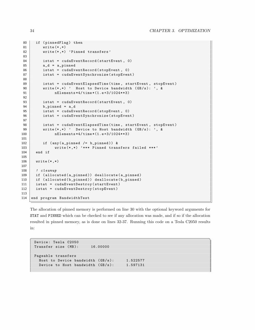
The allocation of pinned memory is performed on line 30 with the optional keyword arguments for
STAT and PINNED which can be checked to see if any allocation was made, and if so if the allocation
resulted in pinned memory, as is done on lines 32-37. Running this code on a Tesla C2050 results
in:
� �Device: Tesla C2050
Transfer size (MB): 16.00000
Pageable transfers
Host to Device bandwidth (GB/s): 1.522577
Device to Host bandwidth (GB/s): 1.597131
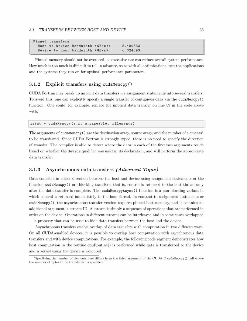
3.1. TRANSFERS BETWEEN HOST AND DEVICE 35
Pinned transfers
Host to Device bandwidth (GB/s): 5.480333
Device to Host bandwidth (GB/s): 6.024593�Pinned memory should not be overused, as excessive use can reduce overall system performance.
How much is too much is difficult to tell in advance, so as with all optimizations, test the applications
and the systems they run on for optimal performance parameters.
3.1.2 Explicit transfers using cudaMemcpy()
CUDA Fortran may break up implicit data transfers via assignment statements into several transfers.
To avoid this, one can explicitly specify a single transfer of contiguous data via the cudaMemcpy()
function. One could, for example, replace the implicit data transfer on line 59 in the code above
with:
istat = cudaMemcpy(a_d , a_pageable , nElements)
The arguments of cudaMemcpy() are the destination array, source array, and the number of elements1
to be transferred. Since CUDA Fortran is strongly typed, there is no need to specify the direction
of transfer. The compiler is able to detect where the data in each of the first two arguments reside
based on whether the device qualifier was used in its declaration, and will perform the appropriate
data transfer.
3.1.3 Asynchronous data transfers (Advanced Topic)
Data transfers in either direction between the host and device using assignment statements or the
function cudaMemcpy() are blocking transfers; that is, control is returned to the host thread only
after the data transfer is complete. The cudaMemcpyAsync() function is a non-blocking variant in
which control is returned immediately to the host thread. In contrast to assignment statements or
cudaMemcpy(), the asynchronous transfer version requires pinned host memory, and it contains an
additional argument, a stream ID. A stream is simply a sequence of operations that are performed in
order on the device. Operations in different streams can be interleaved and in some cases overlapped
— a property that can be used to hide data transfers between the host and the device.
Asynchronous transfers enable overlap of data transfers with computation in two different ways.
On all CUDA-enabled devices, it is possible to overlap host computation with asynchronous data
transfers and with device computations. For example, the following code segment demonstrates how
host computation in the routine cpuRoutine() is performed while data is transferred to the device
and a kernel using the device is executed.
1Specifying the number of elements here differs from the third argument of the CUDA C cudaMemcpy() call wherethe number of bytes to be transferred is specified.
36 CHAPTER 3. OPTIMIZATION
istat = cudaMemcpyAsync(a_d , a_h , nElements , 0)
call kernel <<<gridSize ,blockSize >>>(a_d)
call cpuRoutine(b)
The first three arguments of cudaMemcpyAsync are the same as the three arguments to cudaMemcpy.
The last argument is the stream ID, which in this case uses the default stream, stream 0. The kernel
also uses the default stream, and it will not begin execution until the memory copy completes;
therefore, no explicit synchronization is needed. Because the memory copy and the kernel both
return control to the host immediately, the host subroutine cpuRoutine() can overlap their execution.
In the above example, the memory copy and kernel execution occur sequentially. On devices
that are capable of “concurrent copy and execute,” it is possible to overlap kernel execution on the
device with data transfers between the host and the device. Whether a device has this capability
is indicated by the deviceOverlap field of a cudaDeviceProp variable. On devices that have this
capability, the overlap once again requires pinned host memory, and, in addition, the data transfer
and kernel must use different, non-default streams (streams with non-zero stream IDs). Non-default
streams are required for this overlap because memory copy, memory set functions, and kernel calls
that use the default stream begin only after all preceding calls on the device (in any stream) have
completed, and no operation on the device (in any stream) commences until they are finished.
istat = cudaStreamCreate(stream1)
istat = cudaStreamCreate(stream2)
istat = cudaMemcpyAsync(a_d , a, n, stream1)
call kernel <<<gridSize ,blockSize ,0,stream2 >>>(b_d)
In this code, two streams are created and used in the data transfer and kernel executions as specified
in the last arguments of the cudaMemcpyAsync() call and the kernels execution configuration.2
If the operations on data in a kernel are point-wise, meaning they are independent of other data,
then we can pipeline the data transfers and kernel executions: data can be broken into sections and
transferred in multiple stages, multiple kernels launched to operate on each section as it arrives, and
each section’s results transferred back to the host when the relevant kernel completes. The following
full code listing demonstrates this technique of breaking up data transfers and kernels in order to
hide transfer time:
1 ! This code demonstrates strategies hiding data transfers via
2 ! asynchronous data copies in multiple streams
3
4 module kernels_m
5 contains
2The last two arguments in the execution configuration are optional. The third argument of the execution config-uration relates to shared memory use in the kernel, which we discuss later in this chapter.
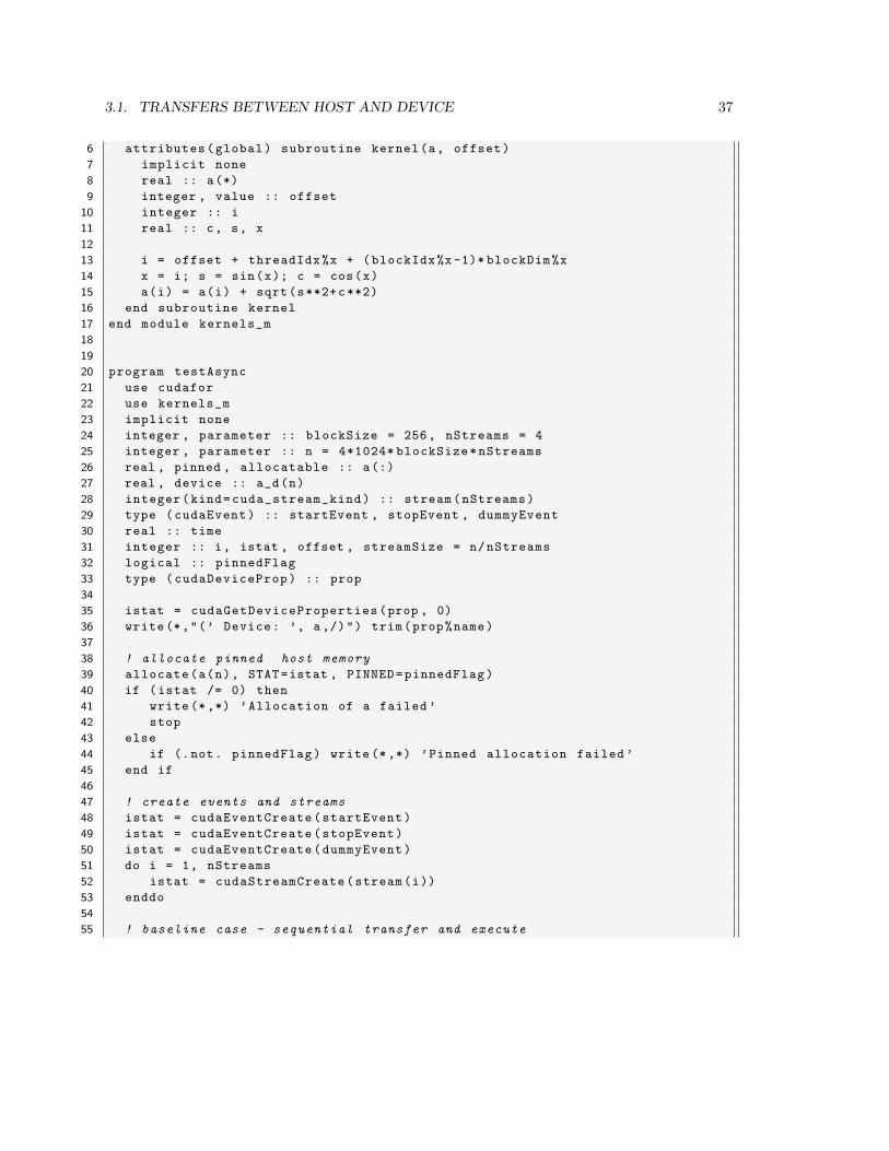
3.1. TRANSFERS BETWEEN HOST AND DEVICE 37
6 attributes(global) subroutine kernel(a, offset)
7 implicit none
8 real :: a(*)
9 integer , value :: offset
10 integer :: i
11 real :: c, s, x
12
13 i = offset + threadIdx%x + (blockIdx%x-1)* blockDim%x
14 x = i; s = sin(x); c = cos(x)
15 a(i) = a(i) + sqrt(s**2+c**2)
16 end subroutine kernel
17 end module kernels_m
18
19
20 program testAsync
21 use cudafor
22 use kernels_m
23 implicit none
24 integer , parameter :: blockSize = 256, nStreams = 4
25 integer , parameter :: n = 4*1024* blockSize*nStreams
26 real , pinned , allocatable :: a(:)
27 real , device :: a_d(n)
28 integer(kind=cuda_stream_kind) :: stream(nStreams)
29 type (cudaEvent) :: startEvent , stopEvent , dummyEvent
30 real :: time
31 integer :: i, istat , offset , streamSize = n/nStreams
32 logical :: pinnedFlag
33 type (cudaDeviceProp) :: prop
34
35 istat = cudaGetDeviceProperties(prop , 0)
36 write(*,"(’ Device: ’, a,/)") trim(prop%name)
37
38 ! allocate pinned host memory
39 allocate(a(n), STAT=istat , PINNED=pinnedFlag)
40 if (istat /= 0) then
41 write (*,*) ’Allocation of a failed ’
42 stop
43 else
44 if (.not. pinnedFlag) write (*,*) ’Pinned allocation failed ’
45 end if
46
47 ! create events and streams
48 istat = cudaEventCreate(startEvent)
49 istat = cudaEventCreate(stopEvent)
50 istat = cudaEventCreate(dummyEvent)
51 do i = 1, nStreams
52 istat = cudaStreamCreate(stream(i))
53 enddo
54
55 ! baseline case - sequential transfer and execute
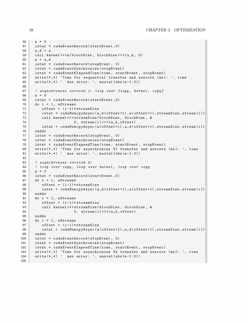
38 CHAPTER 3. OPTIMIZATION
56 a = 0
57 istat = cudaEventRecord(startEvent ,0)
58 a_d = a
59 call kernel <<<n/blockSize , blockSize >>>(a_d , 0)
60 a = a_d
61 istat = cudaEventRecord(stopEvent , 0)
62 istat = cudaEventSynchronize(stopEvent)
63 istat = cudaEventElapsedTime(time , startEvent , stopEvent)
64 write (*,*) ’Time for sequential transfer and execute (ms): ’, time
65 write (*,*) ’ max error: ’, maxval(abs(a -1.0))
66
67 ! asynchronous version 1: loop over {copy , kernel , copy}
68 a = 0
69 istat = cudaEventRecord(startEvent ,0)
70 do i = 1, nStreams
71 offset = (i-1)* streamSize
72 istat = cudaMemcpyAsync(a_d(offset +1),a(offset +1), streamSize ,stream(i))
73 call kernel <<<streamSize/blockSize , blockSize , &
74 0, stream(i)>>>(a_d ,offset)
75 istat = cudaMemcpyAsync(a(offset +1),a_d(offset +1), streamSize ,stream(i))
76 enddo
77 istat = cudaEventRecord(stopEvent , 0)
78 istat = cudaEventSynchronize(stopEvent)
79 istat = cudaEventElapsedTime(time , startEvent , stopEvent)
80 write (*,*) ’Time for asynchronous V1 transfer and execute (ms): ’, time
81 write (*,*) ’ max error: ’, maxval(abs(a -1.0))
82
83 ! asynchronous version 2:
84 ! loop over copy , loop over kernel , loop over copy
85 a = 0
86 istat = cudaEventRecord(startEvent ,0)
87 do i = 1, nStreams
88 offset = (i-1)* streamSize
89 istat = cudaMemcpyAsync(a_d(offset +1),a(offset +1), streamSize ,stream(i))
90 enddo
91 do i = 1, nStreams
92 offset = (i-1)* streamSize
93 call kernel <<<streamSize/blockSize , blockSize , &
94 0, stream(i)>>>(a_d ,offset)
95 enddo
96 do i = 1, nStreams
97 offset = (i-1)* streamSize
98 istat = cudaMemcpyAsync(a(offset +1),a_d(offset +1), streamSize ,stream(i))
99 enddo
100 istat = cudaEventRecord(stopEvent , 0)
101 istat = cudaEventSynchronize(stopEvent)
102 istat = cudaEventElapsedTime(time , startEvent , stopEvent)
103 write (*,*) ’Time for asynchronous V2 transfer and execute (ms): ’, time
104 write (*,*) ’ max error: ’, maxval(abs(a -1.0))
105
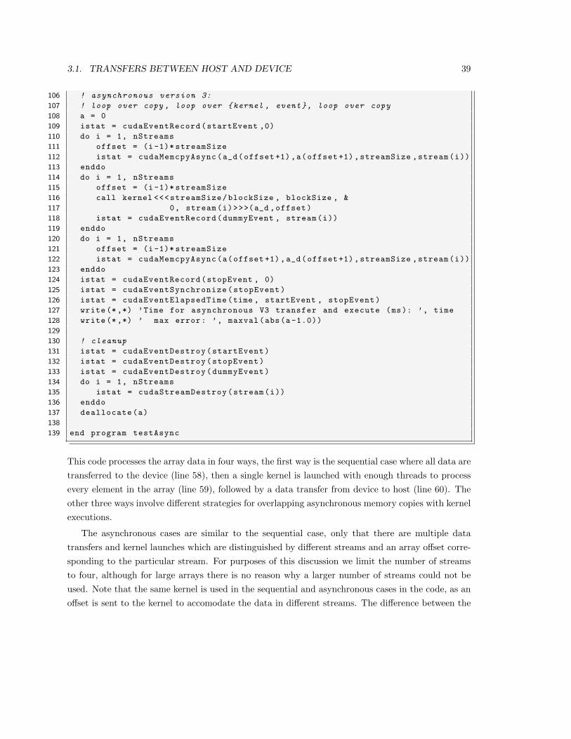
3.1. TRANSFERS BETWEEN HOST AND DEVICE 39
106 ! asynchronous version 3:
107 ! loop over copy , loop over {kernel , event}, loop over copy
108 a = 0
109 istat = cudaEventRecord(startEvent ,0)
110 do i = 1, nStreams
111 offset = (i-1)* streamSize
112 istat = cudaMemcpyAsync(a_d(offset +1),a(offset +1), streamSize ,stream(i))
113 enddo
114 do i = 1, nStreams
115 offset = (i-1)* streamSize
116 call kernel <<<streamSize/blockSize , blockSize , &
117 0, stream(i)>>>(a_d ,offset)
118 istat = cudaEventRecord(dummyEvent , stream(i))
119 enddo
120 do i = 1, nStreams
121 offset = (i-1)* streamSize
122 istat = cudaMemcpyAsync(a(offset +1),a_d(offset +1), streamSize ,stream(i))
123 enddo
124 istat = cudaEventRecord(stopEvent , 0)
125 istat = cudaEventSynchronize(stopEvent)
126 istat = cudaEventElapsedTime(time , startEvent , stopEvent)
127 write (*,*) ’Time for asynchronous V3 transfer and execute (ms): ’, time
128 write (*,*) ’ max error: ’, maxval(abs(a -1.0))
129
130 ! cleanup
131 istat = cudaEventDestroy(startEvent)
132 istat = cudaEventDestroy(stopEvent)
133 istat = cudaEventDestroy(dummyEvent)
134 do i = 1, nStreams
135 istat = cudaStreamDestroy(stream(i))
136 enddo
137 deallocate(a)
138
139 end program testAsync
This code processes the array data in four ways, the first way is the sequential case where all data are
transferred to the device (line 58), then a single kernel is launched with enough threads to process
every element in the array (line 59), followed by a data transfer from device to host (line 60). The
other three ways involve different strategies for overlapping asynchronous memory copies with kernel
executions.
The asynchronous cases are similar to the sequential case, only that there are multiple data
transfers and kernel launches which are distinguished by different streams and an array offset corre-
sponding to the particular stream. For purposes of this discussion we limit the number of streams
to four, although for large arrays there is no reason why a larger number of streams could not be
used. Note that the same kernel is used in the sequential and asynchronous cases in the code, as an
offset is sent to the kernel to accomodate the data in different streams. The difference between the

40 CHAPTER 3. OPTIMIZATION
first two asynchronous versions is the order in which the copies and kernels are executed. The first
version (starting on line 67) loops over each stream where each stream issues a host-to-device copy,
a kernel, and a device-to-host copy. The second version (starting on line 83) issues all host-to-device
copies, then all kernel launches, and then all device-to-host copies. The third asynchronous version
(starting on line 106) is the same as the second version except that a dummy event is recorded after
each kernel is issued in the same stream as the kernel.
At this point you may be asking why we have three versions of the asynchronous case. The
reason is that these variants perform differently on different hardware. Running this code on the
NVIDIA Tesla C1060 produces:� �Device: Tesla C1060
Time for sequential transfer and execute (ms): 12.92381
max error: 2.3841858E-07
Time for asynchronous V1 transfer and execute (ms): 13.63690
max error: 2.3841858E-07
Time for asynchronous V2 transfer and execute (ms): 8.845888
max error: 2.3841858E-07
Time for asynchronous V3 transfer and execute (ms): 8.998560
max error: 2.3841858E-07�and on the NVIDIA Tesla C2050 we get:� �
Device: Tesla C2050
Time for sequential transfer and execute (ms): 9.984512
max error: 1.1920929E-07
Time for asynchronous V1 transfer and execute (ms): 5.735584
max error: 1.1920929E-07
Time for asynchronous V2 transfer and execute (ms): 7.597984
max error: 1.1920929E-07
Time for asynchronous V3 transfer and execute (ms): 5.735424
max error: 1.1920929E-07�To decipher these results we need to understand a bit more about how devices schedule and
execute various tasks. CUDA devices contain engines for various tasks, and operations are queued up
in these engines as they are issued. Dependencies between tasks in different engines are maintained,
but within any engine all dependence is lost, as tasks in an engine’s queue are executed in the order
they are issued by the host thread. For example, the C1060 has a single copy engine and a single
kernel engine. For the above code, time lines for the execution on the device is schematically shown
in the top diagram of Figure 3.1. In this schematic we have assumed that the time required for the
host-to-device transfer, kernel execution, and device-to-host transfer are approximately the same
(the kernel code was chosen in order to make these times comparable). For the sequential kernel,
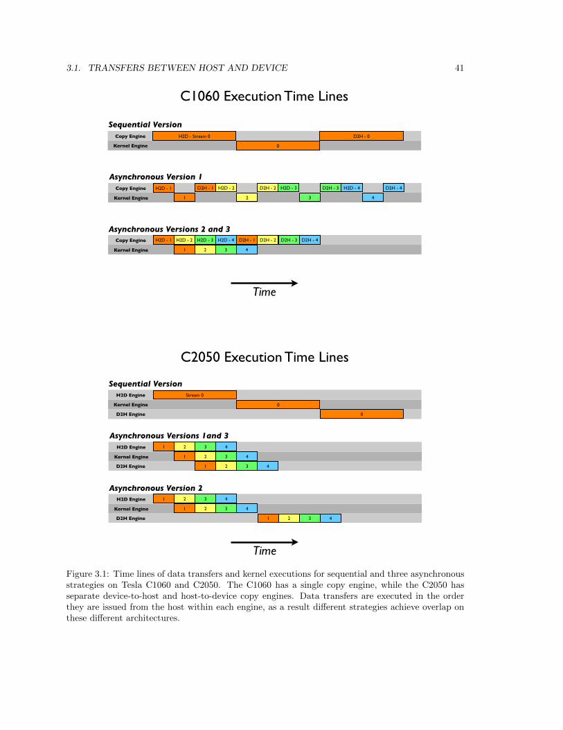
3.1. TRANSFERS BETWEEN HOST AND DEVICE 41
H2D - Stream 0
0
D2H - 0
Kernel Engine
Copy Engine
H2D - 1
1Kernel Engine
Copy Engine D2H - 1 H2D - 2
2
D2H - 2 H2D - 3
3
D2H - 3 H2D - 4
4
D2H - 4
H2D - 1
1Kernel Engine
Copy Engine D2H - 1H2D - 2
2
D2H - 2H2D - 3
3
D2H - 3H2D - 4
4
D2H - 4
C1060 Execution Time Lines
Sequential Version
Asynchronous Version 1
Asynchronous Versions 2 and 3
Time
C2050 Execution Time Lines
Sequential Version
Asynchronous Versions 1and 3
Asynchronous Version 2
Time
Stream 0
0Kernel Engine
H2D Engine
D2H Engine 0
1
1Kernel Engine
H2D Engine 2
2
3
3
4
4
D2H Engine 1 2 3 4
1
1Kernel Engine
H2D Engine 2
2
3
3
4
4
D2H Engine 1 2 3 4
Figure 3.1: Time lines of data transfers and kernel executions for sequential and three asynchronousstrategies on Tesla C1060 and C2050. The C1060 has a single copy engine, while the C2050 hasseparate device-to-host and host-to-device copy engines. Data transfers are executed in the orderthey are issued from the host within each engine, as a result different strategies achieve overlap onthese different architectures.
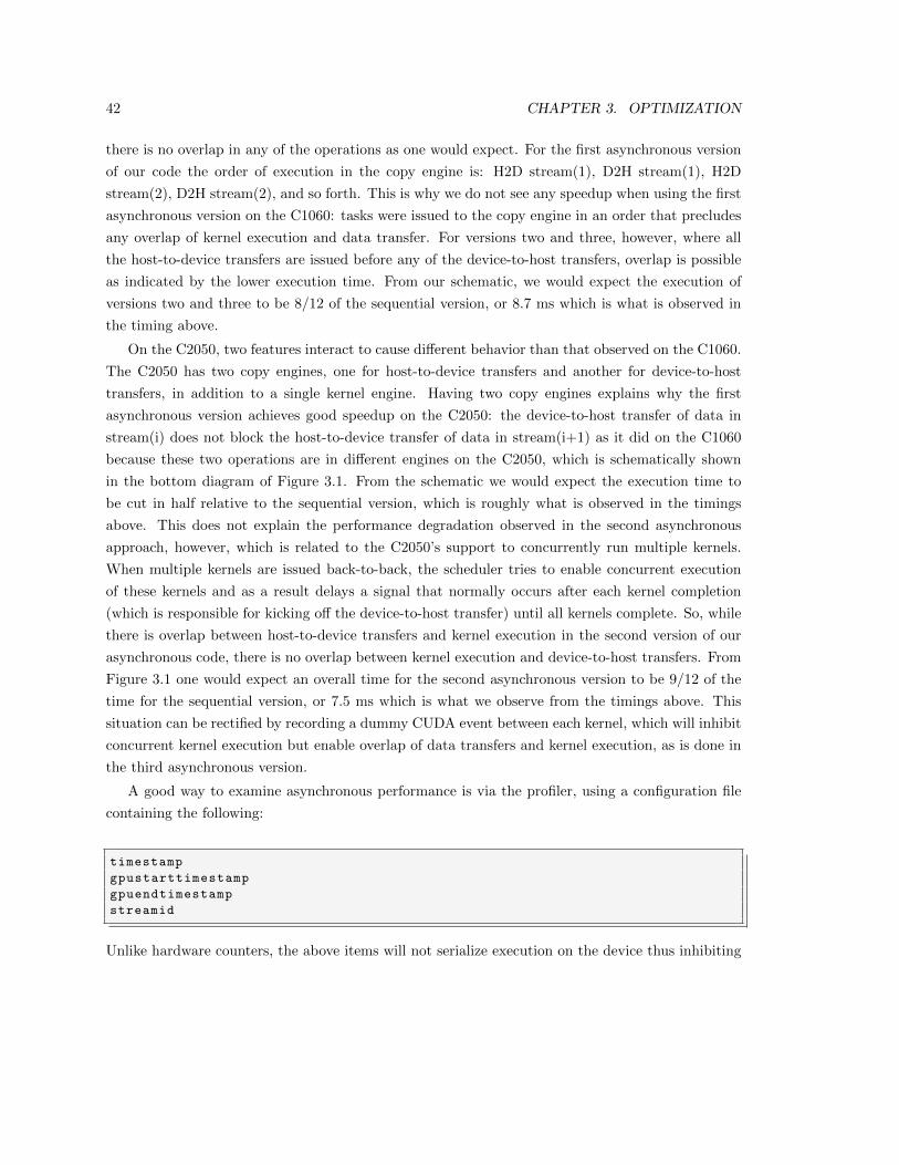
42 CHAPTER 3. OPTIMIZATION
there is no overlap in any of the operations as one would expect. For the first asynchronous version
of our code the order of execution in the copy engine is: H2D stream(1), D2H stream(1), H2D
stream(2), D2H stream(2), and so forth. This is why we do not see any speedup when using the first
asynchronous version on the C1060: tasks were issued to the copy engine in an order that precludes
any overlap of kernel execution and data transfer. For versions two and three, however, where all
the host-to-device transfers are issued before any of the device-to-host transfers, overlap is possible
as indicated by the lower execution time. From our schematic, we would expect the execution of
versions two and three to be 8/12 of the sequential version, or 8.7 ms which is what is observed in
the timing above.
On the C2050, two features interact to cause different behavior than that observed on the C1060.
The C2050 has two copy engines, one for host-to-device transfers and another for device-to-host
transfers, in addition to a single kernel engine. Having two copy engines explains why the first
asynchronous version achieves good speedup on the C2050: the device-to-host transfer of data in
stream(i) does not block the host-to-device transfer of data in stream(i+1) as it did on the C1060
because these two operations are in different engines on the C2050, which is schematically shown
in the bottom diagram of Figure 3.1. From the schematic we would expect the execution time to
be cut in half relative to the sequential version, which is roughly what is observed in the timings
above. This does not explain the performance degradation observed in the second asynchronous
approach, however, which is related to the C2050’s support to concurrently run multiple kernels.
When multiple kernels are issued back-to-back, the scheduler tries to enable concurrent execution
of these kernels and as a result delays a signal that normally occurs after each kernel completion
(which is responsible for kicking off the device-to-host transfer) until all kernels complete. So, while
there is overlap between host-to-device transfers and kernel execution in the second version of our
asynchronous code, there is no overlap between kernel execution and device-to-host transfers. From
Figure 3.1 one would expect an overall time for the second asynchronous version to be 9/12 of the
time for the sequential version, or 7.5 ms which is what we observe from the timings above. This
situation can be rectified by recording a dummy CUDA event between each kernel, which will inhibit
concurrent kernel execution but enable overlap of data transfers and kernel execution, as is done in
the third asynchronous version.
A good way to examine asynchronous performance is via the profiler, using a configuration file
containing the following:
timestamp
gpustarttimestamp
gpuendtimestamp
streamid
Unlike hardware counters, the above items will not serialize execution on the device thus inhibiting
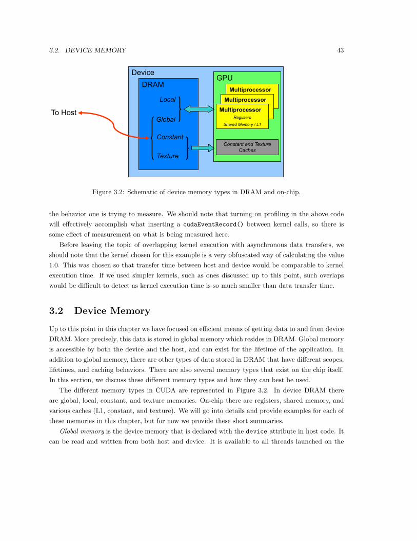
3.2. DEVICE MEMORY 43
DeviceDRAM
Global
Constant
Texture
Local
GPUMultiprocessor
Registers
Shared MemoryMultiprocessor
Registers
Shared MemoryMultiprocessor
Registers
Shared Memory / L1
Constant and Texture Caches
To Host
Figure 3.2: Schematic of device memory types in DRAM and on-chip.
the behavior one is trying to measure. We should note that turning on profiling in the above code
will effectively accomplish what inserting a cudaEventRecord() between kernel calls, so there is
some effect of measurement on what is being measured here.
Before leaving the topic of overlapping kernel execution with asynchronous data transfers, we
should note that the kernel chosen for this example is a very obfuscated way of calculating the value
1.0. This was chosen so that transfer time between host and device would be comparable to kernel
execution time. If we used simpler kernels, such as ones discussed up to this point, such overlaps
would be difficult to detect as kernel execution time is so much smaller than data transfer time.
3.2 Device Memory
Up to this point in this chapter we have focused on efficient means of getting data to and from device
DRAM. More precisely, this data is stored in global memory which resides in DRAM. Global memory
is accessible by both the device and the host, and can exist for the lifetime of the application. In
addition to global memory, there are other types of data stored in DRAM that have different scopes,
lifetimes, and caching behaviors. There are also several memory types that exist on the chip itself.
In this section, we discuss these different memory types and how they can best be used.
The different memory types in CUDA are represented in Figure 3.2. In device DRAM there
are global, local, constant, and texture memories. On-chip there are registers, shared memory, and
various caches (L1, constant, and texture). We will go into details and provide examples for each of
these memories in this chapter, but for now we provide these short summaries.
Global memory is the device memory that is declared with the device attribute in host code. It
can be read and written from both host and device. It is available to all threads launched on the
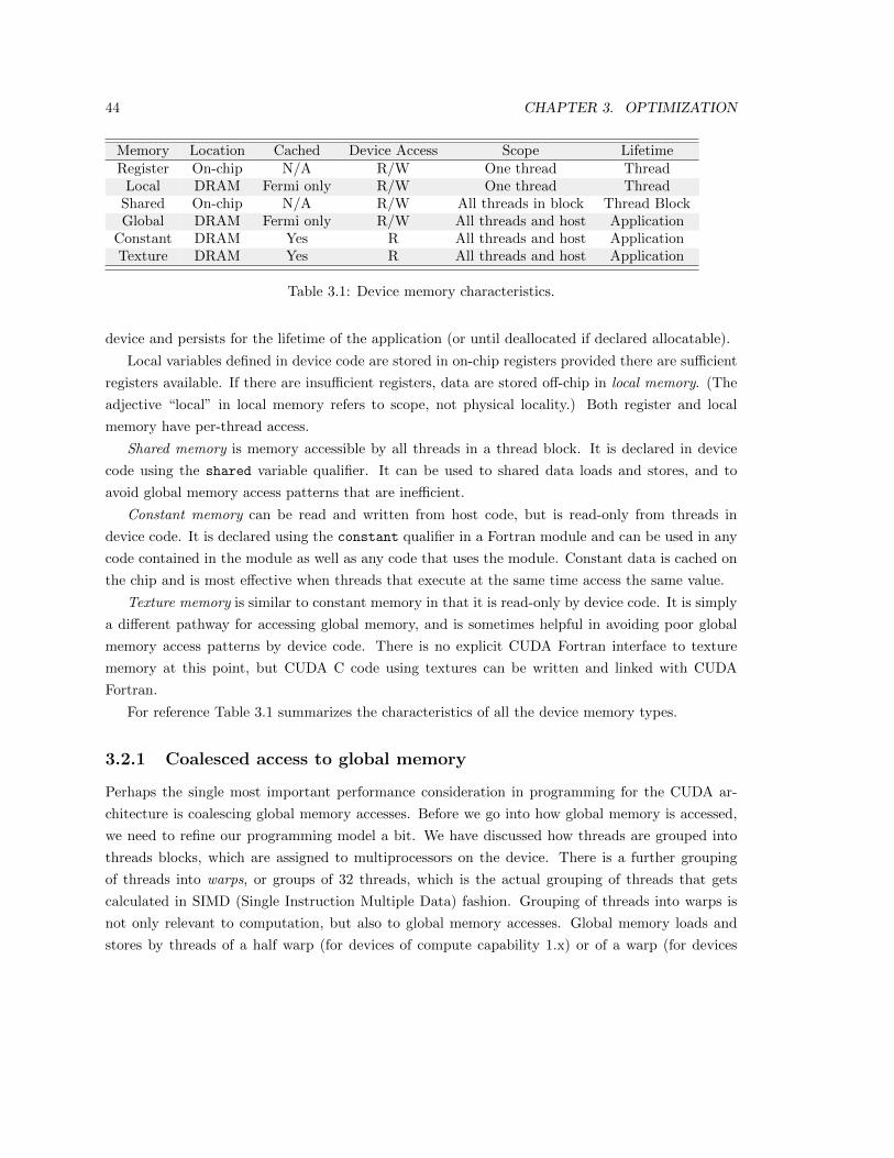
44 CHAPTER 3. OPTIMIZATION
Memory Location Cached Device Access Scope LifetimeRegister On-chip N/A R/W One thread Thread
Local DRAM Fermi only R/W One thread ThreadShared On-chip N/A R/W All threads in block Thread BlockGlobal DRAM Fermi only R/W All threads and host Application
Constant DRAM Yes R All threads and host ApplicationTexture DRAM Yes R All threads and host Application
Table 3.1: Device memory characteristics.
device and persists for the lifetime of the application (or until deallocated if declared allocatable).
Local variables defined in device code are stored in on-chip registers provided there are sufficient
registers available. If there are insufficient registers, data are stored off-chip in local memory. (The
adjective “local” in local memory refers to scope, not physical locality.) Both register and local
memory have per-thread access.
Shared memory is memory accessible by all threads in a thread block. It is declared in device
code using the shared variable qualifier. It can be used to shared data loads and stores, and to
avoid global memory access patterns that are inefficient.
Constant memory can be read and written from host code, but is read-only from threads in
device code. It is declared using the constant qualifier in a Fortran module and can be used in any
code contained in the module as well as any code that uses the module. Constant data is cached on
the chip and is most effective when threads that execute at the same time access the same value.
Texture memory is similar to constant memory in that it is read-only by device code. It is simply
a different pathway for accessing global memory, and is sometimes helpful in avoiding poor global
memory access patterns by device code. There is no explicit CUDA Fortran interface to texture
memory at this point, but CUDA C code using textures can be written and linked with CUDA
Fortran.
For reference Table 3.1 summarizes the characteristics of all the device memory types.
3.2.1 Coalesced access to global memory
Perhaps the single most important performance consideration in programming for the CUDA ar-
chitecture is coalescing global memory accesses. Before we go into how global memory is accessed,
we need to refine our programming model a bit. We have discussed how threads are grouped into
threads blocks, which are assigned to multiprocessors on the device. There is a further grouping
of threads into warps, or groups of 32 threads, which is the actual grouping of threads that gets
calculated in SIMD (Single Instruction Multiple Data) fashion. Grouping of threads into warps is
not only relevant to computation, but also to global memory accesses. Global memory loads and
stores by threads of a half warp (for devices of compute capability 1.x) or of a warp (for devices
3.2. DEVICE MEMORY 45
of compute capability 2.x) are coalesced by the device into as few as one transaction when certain
access requirements are met. To understand these access requirements and how they evolved with
different Tesla architectures we run some simple experiments on three Tesla cards, a C870 (compute
capability 1.0), a C1060 (compute capability 1.3), and a C2050 (compute capability 2.0), in both
single and double precision (when possible).
We run two experiments that are variants of our increment kernel, one with an array offset or
misaligned access of the array, and the other performs strided access in a similar fashion. The code
that performs this is:
1 module kernels_m
2 use precision_m
3 contains
4 attributes(global) subroutine offset(a, s)
5 real(fp_kind) :: a(*)
6 integer , value :: s
7 integer :: i
8 i = blockDim%x*( blockIdx%x-1)+ threadIdx%x + s
9 a(i) = a(i)+1
10 end subroutine offset
11
12 attributes(global) subroutine stride(a, s)
13 real(fp_kind) :: a(*)
14 integer , value :: s
15 integer :: i
16 i = (blockDim%x*( blockIdx%x-1)+ threadIdx%x) * s
17 a(i) = a(i)+1
18 end subroutine stride
19 end module kernels_m
20
21 program offsetNStride
22 use cudafor
23 use kernels_m
24
25 implicit none
26
27 integer , parameter :: nMB = 4 ! NB: arrays are 33*nMB MB for stride cases
28 integer , parameter :: blockSize = 256
29 integer :: n
30 real(fp_kind), device , allocatable :: a_d(:), b_d (:)
31 type(cudaEvent) :: startEvent , stopEvent
32 type(cudaDeviceProp) :: prop
33 integer :: i, istat
34 real (4) :: time
35
36
37 istat = cudaGetDeviceProperties(prop , 0)
38 write(*,’(/," Device: ",a)’) trim(prop%name)
46 CHAPTER 3. OPTIMIZATION
39 write(*,’(" Transfer size (MB): ",i0)’) nMB
40
41 if (kind(a_d) == singlePrecision) then
42 write(*,’(a,/)’) ’Single Precision ’
43 else
44 write(*,’(a,/)’) ’Double Precision ’
45 endif
46 n = nMB *1024*1024/ fp_kind
47 allocate(a_d(n*33), b_d(n*33))
48
49
50 istat = cudaEventCreate(startEvent)
51 istat = cudaEventCreate(stopEvent)
52
53 write (*,*) ’Offset , Bandwidth (GB/s):’
54 call offset <<<n/blockSize ,blockSize >>>(b_d , 0)
55 do i = 0, 32
56 a_d = 0.0
57 istat = cudaEventRecord(startEvent ,0)
58 call offset <<<n/blockSize ,blockSize >>>(a_d , i)
59 istat = cudaEventRecord(stopEvent ,0)
60 istat = cudaEventSynchronize(stopEvent)
61
62 istat = cudaEventElapsedTime(time , startEvent , stopEvent)
63 write (*,*) i, 2*nMB/time *(1.e+3/1024)
64 enddo
65
66 write (*,*)
67 write (*,*) ’Stride , Bandwidth (GB/s):’
68 call stride <<<n/blockSize ,blockSize >>>(b_d , 1)
69 do i = 1, 32
70 a_d = 0.0
71 istat = cudaEventRecord(startEvent ,0)
72 call stride <<<n/blockSize ,blockSize >>>(a_d , i)
73 istat = cudaEventRecord(stopEvent ,0)
74 istat = cudaEventSynchronize(stopEvent)
75 istat = cudaEventElapsedTime(time , startEvent , stopEvent)
76 write (*,*) i, 2*nMB/time *(1.e+3/1024)
77 enddo
78
79 istat = cudaEventDestroy(startEvent)
80 istat = cudaEventDestroy(stopEvent)
81 deallocate(a_d , b_d)
82
83 end program offsetNStride
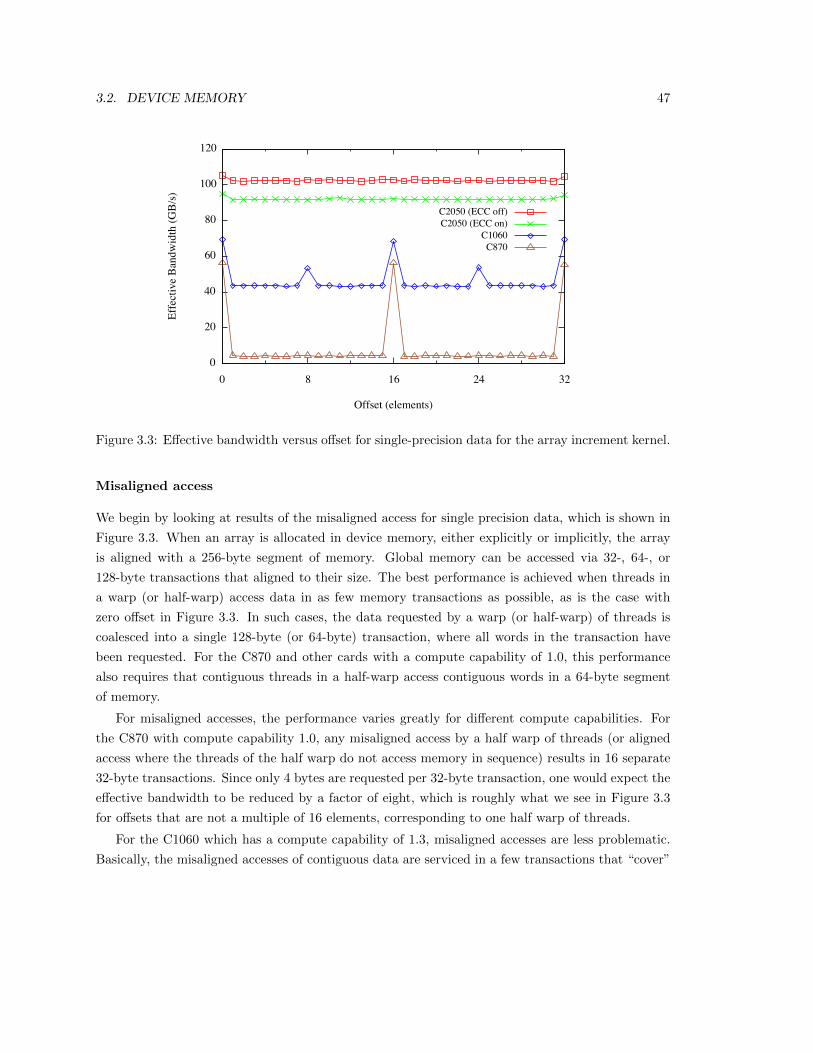
3.2. DEVICE MEMORY 47
Figure 3.3: Effective bandwidth versus offset for single-precision data for the array increment kernel.
Misaligned access
We begin by looking at results of the misaligned access for single precision data, which is shown in
Figure 3.3. When an array is allocated in device memory, either explicitly or implicitly, the array
is aligned with a 256-byte segment of memory. Global memory can be accessed via 32-, 64-, or
128-byte transactions that aligned to their size. The best performance is achieved when threads in
a warp (or half-warp) access data in as few memory transactions as possible, as is the case with
zero offset in Figure 3.3. In such cases, the data requested by a warp (or half-warp) of threads is
coalesced into a single 128-byte (or 64-byte) transaction, where all words in the transaction have
been requested. For the C870 and other cards with a compute capability of 1.0, this performance
also requires that contiguous threads in a half-warp access contiguous words in a 64-byte segment
of memory.
For misaligned accesses, the performance varies greatly for different compute capabilities. For
the C870 with compute capability 1.0, any misaligned access by a half warp of threads (or aligned
access where the threads of the half warp do not access memory in sequence) results in 16 separate
32-byte transactions. Since only 4 bytes are requested per 32-byte transaction, one would expect the
effective bandwidth to be reduced by a factor of eight, which is roughly what we see in Figure 3.3
for offsets that are not a multiple of 16 elements, corresponding to one half warp of threads.
For the C1060 which has a compute capability of 1.3, misaligned accesses are less problematic.
Basically, the misaligned accesses of contiguous data are serviced in a few transactions that “cover”
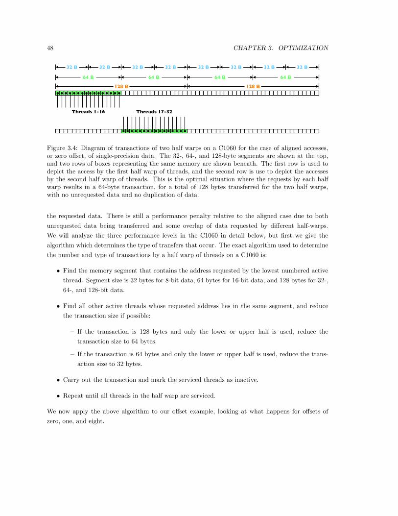
48 CHAPTER 3. OPTIMIZATION
64 B 64 B 64 B 64 B
128 B128 B
Threads 1-16
32 B 32 B 32 B 32 B 32 B 32 B 32 B 32 B
Threads 17-32
Figure 3.4: Diagram of transactions of two half warps on a C1060 for the case of aligned accesses,or zero offset, of single-precision data. The 32-, 64-, and 128-byte segments are shown at the top,and two rows of boxes representing the same memory are shown beneath. The first row is used todepict the access by the first half warp of threads, and the second row is use to depict the accessesby the second half warp of threads. This is the optimal situation where the requests by each halfwarp results in a 64-byte transaction, for a total of 128 bytes transferred for the two half warps,with no unrequested data and no duplication of data.
the requested data. There is still a performance penalty relative to the aligned case due to both
unrequested data being transferred and some overlap of data requested by different half-warps.
We will analyze the three performance levels in the C1060 in detail below, but first we give the
algorithm which determines the type of transfers that occur. The exact algorithm used to determine
the number and type of transactions by a half warp of threads on a C1060 is:
• Find the memory segment that contains the address requested by the lowest numbered active
thread. Segment size is 32 bytes for 8-bit data, 64 bytes for 16-bit data, and 128 bytes for 32-,
64-, and 128-bit data.
• Find all other active threads whose requested address lies in the same segment, and reduce
the transaction size if possible:
– If the transaction is 128 bytes and only the lower or upper half is used, reduce the
transaction size to 64 bytes.
– If the transaction is 64 bytes and only the lower or upper half is used, reduce the trans-
action size to 32 bytes.
• Carry out the transaction and mark the serviced threads as inactive.
• Repeat until all threads in the half warp are serviced.
We now apply the above algorithm to our offset example, looking at what happens for offsets of
zero, one, and eight.
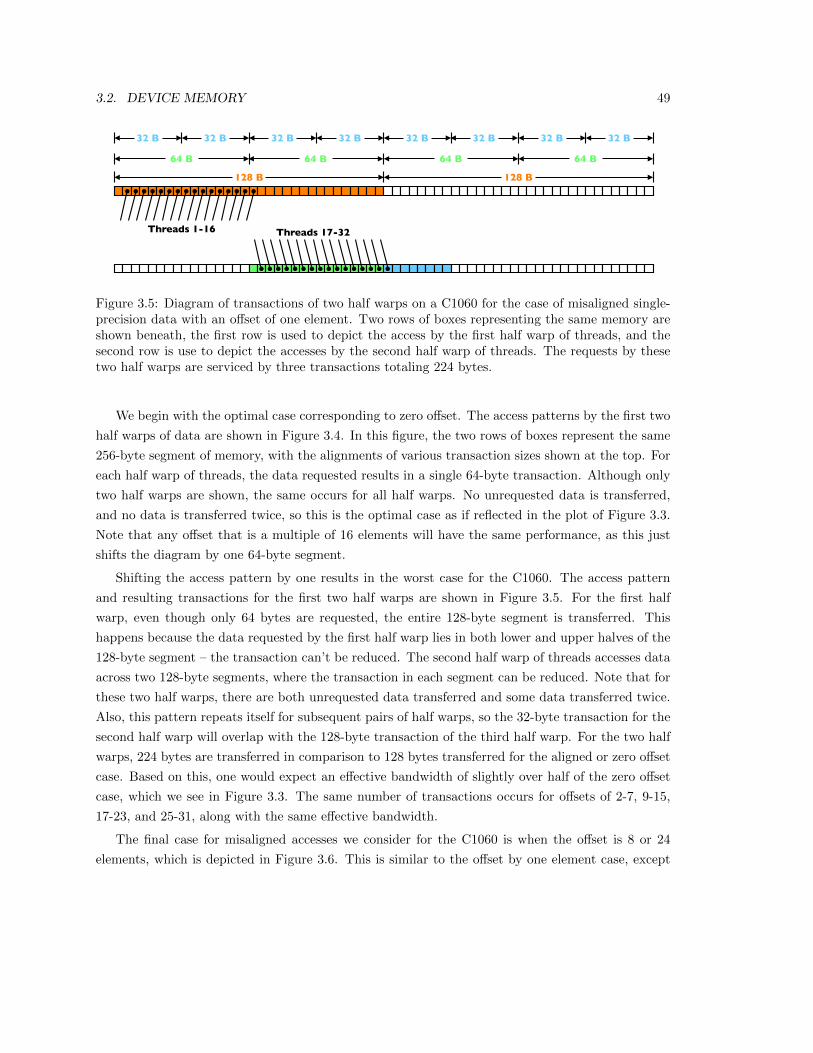
3.2. DEVICE MEMORY 49
64 B 64 B 64 B 64 B
128 B128 B
Threads 1-16
32 B 32 B 32 B 32 B 32 B 32 B 32 B 32 B
Threads 17-32
Figure 3.5: Diagram of transactions of two half warps on a C1060 for the case of misaligned single-precision data with an offset of one element. Two rows of boxes representing the same memory areshown beneath, the first row is used to depict the access by the first half warp of threads, and thesecond row is use to depict the accesses by the second half warp of threads. The requests by thesetwo half warps are serviced by three transactions totaling 224 bytes.
We begin with the optimal case corresponding to zero offset. The access patterns by the first two
half warps of data are shown in Figure 3.4. In this figure, the two rows of boxes represent the same
256-byte segment of memory, with the alignments of various transaction sizes shown at the top. For
each half warp of threads, the data requested results in a single 64-byte transaction. Although only
two half warps are shown, the same occurs for all half warps. No unrequested data is transferred,
and no data is transferred twice, so this is the optimal case as if reflected in the plot of Figure 3.3.
Note that any offset that is a multiple of 16 elements will have the same performance, as this just
shifts the diagram by one 64-byte segment.
Shifting the access pattern by one results in the worst case for the C1060. The access pattern
and resulting transactions for the first two half warps are shown in Figure 3.5. For the first half
warp, even though only 64 bytes are requested, the entire 128-byte segment is transferred. This
happens because the data requested by the first half warp lies in both lower and upper halves of the
128-byte segment – the transaction can’t be reduced. The second half warp of threads accesses data
across two 128-byte segments, where the transaction in each segment can be reduced. Note that for
these two half warps, there are both unrequested data transferred and some data transferred twice.
Also, this pattern repeats itself for subsequent pairs of half warps, so the 32-byte transaction for the
second half warp will overlap with the 128-byte transaction of the third half warp. For the two half
warps, 224 bytes are transferred in comparison to 128 bytes transferred for the aligned or zero offset
case. Based on this, one would expect an effective bandwidth of slightly over half of the zero offset
case, which we see in Figure 3.3. The same number of transactions occurs for offsets of 2-7, 9-15,
17-23, and 25-31, along with the same effective bandwidth.
The final case for misaligned accesses we consider for the C1060 is when the offset is 8 or 24
elements, which is depicted in Figure 3.6. This is similar to the offset by one element case, except
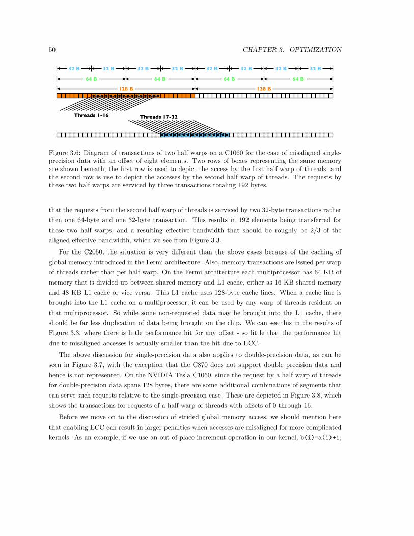
50 CHAPTER 3. OPTIMIZATION
64 B 64 B 64 B 64 B
128 B128 B
Threads 1-16
32 B 32 B 32 B 32 B 32 B 32 B 32 B 32 B
Threads 17-32
Figure 3.6: Diagram of transactions of two half warps on a C1060 for the case of misaligned single-precision data with an offset of eight elements. Two rows of boxes representing the same memoryare shown beneath, the first row is used to depict the access by the first half warp of threads, andthe second row is use to depict the accesses by the second half warp of threads. The requests bythese two half warps are serviced by three transactions totaling 192 bytes.
that the requests from the second half warp of threads is serviced by two 32-byte transactions rather
then one 64-byte and one 32-byte transaction. This results in 192 elements being transferred for
these two half warps, and a resulting effective bandwidth that should be roughly be 2/3 of the
aligned effective bandwidth, which we see from Figure 3.3.
For the C2050, the situation is very different than the above cases because of the caching of
global memory introduced in the Fermi architecture. Also, memory transactions are issued per warp
of threads rather than per half warp. On the Fermi architecture each multiprocessor has 64 KB of
memory that is divided up between shared memory and L1 cache, either as 16 KB shared memory
and 48 KB L1 cache or vice versa. This L1 cache uses 128-byte cache lines. When a cache line is
brought into the L1 cache on a multiprocessor, it can be used by any warp of threads resident on
that multiprocessor. So while some non-requested data may be brought into the L1 cache, there
should be far less duplication of data being brought on the chip. We can see this in the results of
Figure 3.3, where there is little performance hit for any offset - so little that the performance hit
due to misaligned accesses is actually smaller than the hit due to ECC.
The above discussion for single-precision data also applies to double-precision data, as can be
seen in Figure 3.7, with the exception that the C870 does not support double precision data and
hence is not represented. On the NVIDIA Tesla C1060, since the request by a half warp of threads
for double-precision data spans 128 bytes, there are some additional combinations of segments that
can serve such requests relative to the single-precision case. These are depicted in Figure 3.8, which
shows the transactions for requests of a half warp of threads with offsets of 0 through 16.
Before we move on to the discussion of strided global memory access, we should mention here
that enabling ECC can result in larger penalties when accesses are misaligned for more complicated
kernels. As an example, if we use an out-of-place increment operation in our kernel, b(i)=a(i)+1,
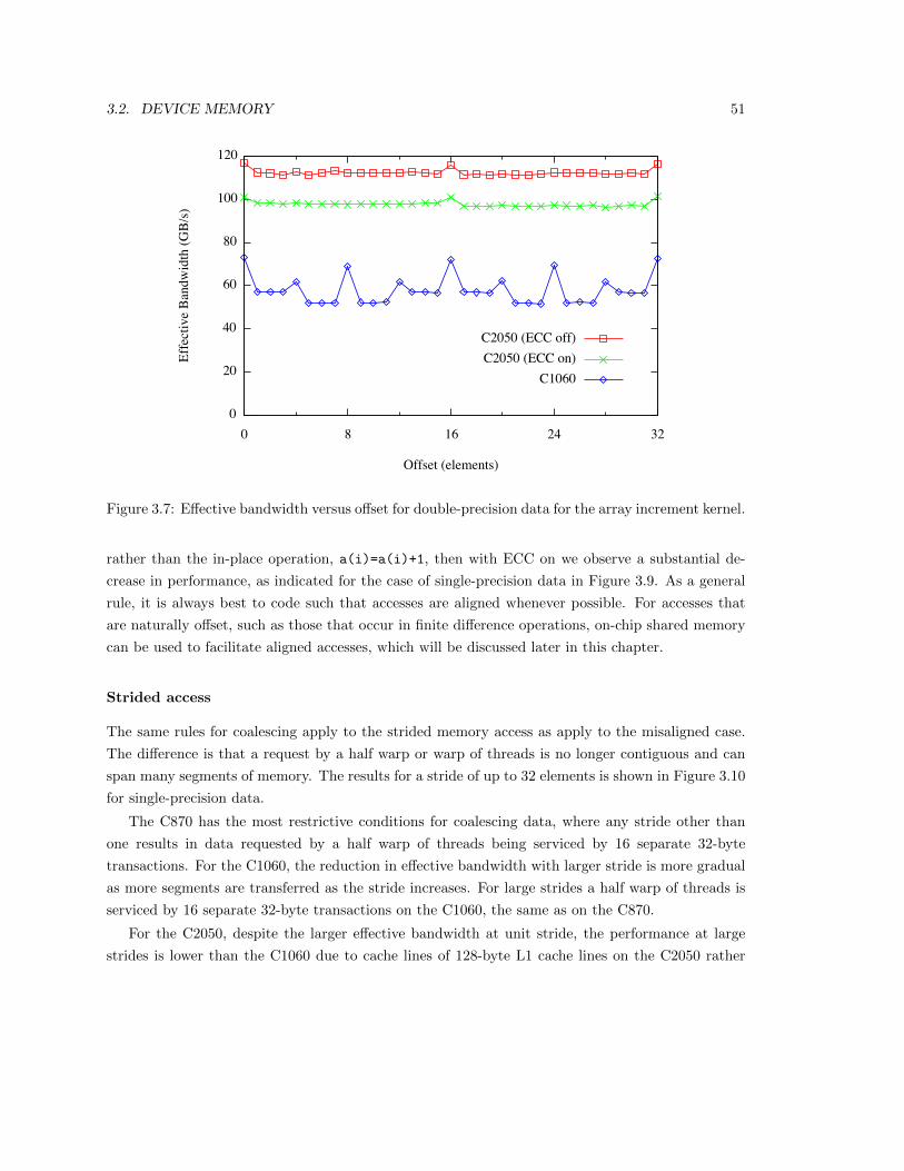
3.2. DEVICE MEMORY 51
Figure 3.7: Effective bandwidth versus offset for double-precision data for the array increment kernel.
rather than the in-place operation, a(i)=a(i)+1, then with ECC on we observe a substantial de-
crease in performance, as indicated for the case of single-precision data in Figure 3.9. As a general
rule, it is always best to code such that accesses are aligned whenever possible. For accesses that
are naturally offset, such as those that occur in finite difference operations, on-chip shared memory
can be used to facilitate aligned accesses, which will be discussed later in this chapter.
Strided access
The same rules for coalescing apply to the strided memory access as apply to the misaligned case.
The difference is that a request by a half warp or warp of threads is no longer contiguous and can
span many segments of memory. The results for a stride of up to 32 elements is shown in Figure 3.10
for single-precision data.
The C870 has the most restrictive conditions for coalescing data, where any stride other than
one results in data requested by a half warp of threads being serviced by 16 separate 32-byte
transactions. For the C1060, the reduction in effective bandwidth with larger stride is more gradual
as more segments are transferred as the stride increases. For large strides a half warp of threads is
serviced by 16 separate 32-byte transactions on the C1060, the same as on the C870.
For the C2050, despite the larger effective bandwidth at unit stride, the performance at large
strides is lower than the C1060 due to cache lines of 128-byte L1 cache lines on the C2050 rather
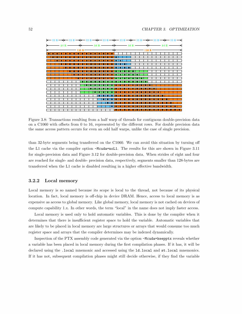
52 CHAPTER 3. OPTIMIZATION
64 B 64 B 64 B 64 B
128 B128 B
32 B 32 B 32 B 32 B 32 B 32 B 32 B 32 B
Figure 3.8: Transactions resulting from a half warp of threads for contiguous double-precision dataon a C1060 with offsets from 0 to 16, represented by the different rows. For double precision datathe same access pattern occurs for even an odd half warps, unlike the case of single precision.
than 32-byte segments being transferred on the C1060. We can avoid this situation by turning off
the L1 cache via the compiler option -Mcuda=noL1. The results for this are shown in Figure 3.11
for single-precision data and Figure 3.12 for double-precision data. When strides of eight and four
are reached for single- and double- precision data, respectively, segments smaller than 128-bytes are
transferred when the L1 cache is disabled resulting in a higher effective bandwidth.
3.2.2 Local memory
Local memory is so named because its scope is local to the thread, not because of its physical
location. In fact, local memory is off-chip in device DRAM. Hence, access to local memory is as
expensive as access to global memory. Like global memory, local memory is not cached on devices of
compute capability 1.x. In other words, the term “local” in the name does not imply faster access.
Local memory is used only to hold automatic variables. This is done by the compiler when it
determines that there is insufficient register space to hold the variable. Automatic variables that
are likely to be placed in local memory are large structures or arrays that would consume too much
register space and arrays that the compiler determines may be indexed dynamically.
Inspection of the PTX assembly code generated via the option -Mcuda=keepptx reveals whether
a variable has been placed in local memory during the first compilation phases. If it has, it will be
declared using the .local mnemonic and accessed using the ld.local and st.local mnemonics.
If it has not, subsequent compilation phases might still decide otherwise, if they find the variable
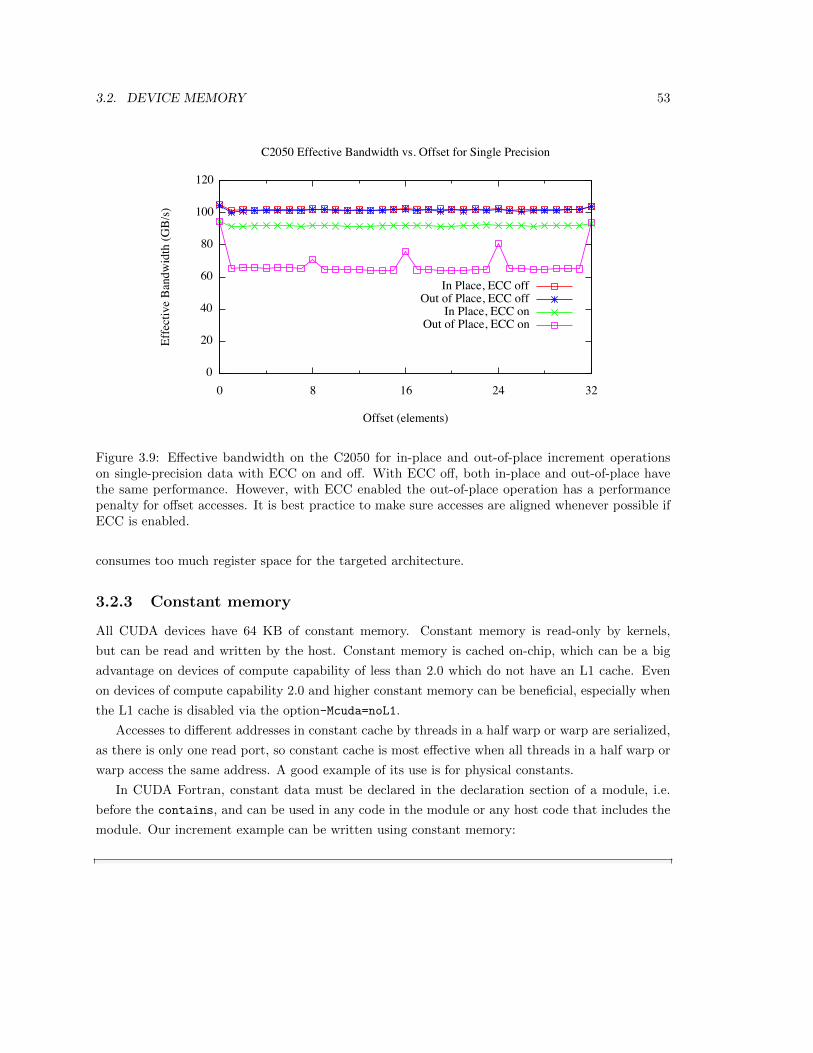
3.2. DEVICE MEMORY 53
Figure 3.9: Effective bandwidth on the C2050 for in-place and out-of-place increment operationson single-precision data with ECC on and off. With ECC off, both in-place and out-of-place havethe same performance. However, with ECC enabled the out-of-place operation has a performancepenalty for offset accesses. It is best practice to make sure accesses are aligned whenever possible ifECC is enabled.
consumes too much register space for the targeted architecture.
3.2.3 Constant memory
All CUDA devices have 64 KB of constant memory. Constant memory is read-only by kernels,
but can be read and written by the host. Constant memory is cached on-chip, which can be a big
advantage on devices of compute capability of less than 2.0 which do not have an L1 cache. Even
on devices of compute capability 2.0 and higher constant memory can be beneficial, especially when
the L1 cache is disabled via the option-Mcuda=noL1.
Accesses to different addresses in constant cache by threads in a half warp or warp are serialized,
as there is only one read port, so constant cache is most effective when all threads in a half warp or
warp access the same address. A good example of its use is for physical constants.
In CUDA Fortran, constant data must be declared in the declaration section of a module, i.e.
before the contains, and can be used in any code in the module or any host code that includes the
module. Our increment example can be written using constant memory:
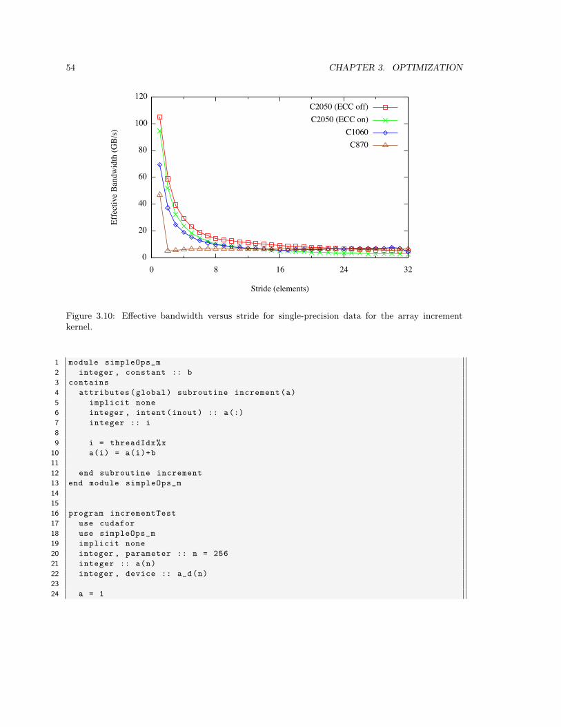
54 CHAPTER 3. OPTIMIZATION
Figure 3.10: Effective bandwidth versus stride for single-precision data for the array incrementkernel.
1 module simpleOps_m
2 integer , constant :: b
3 contains
4 attributes(global) subroutine increment(a)
5 implicit none
6 integer , intent(inout) :: a(:)
7 integer :: i
8
9 i = threadIdx%x
10 a(i) = a(i)+b
11
12 end subroutine increment
13 end module simpleOps_m
14
15
16 program incrementTest
17 use cudafor
18 use simpleOps_m
19 implicit none
20 integer , parameter :: n = 256
21 integer :: a(n)
22 integer , device :: a_d(n)
23
24 a = 1
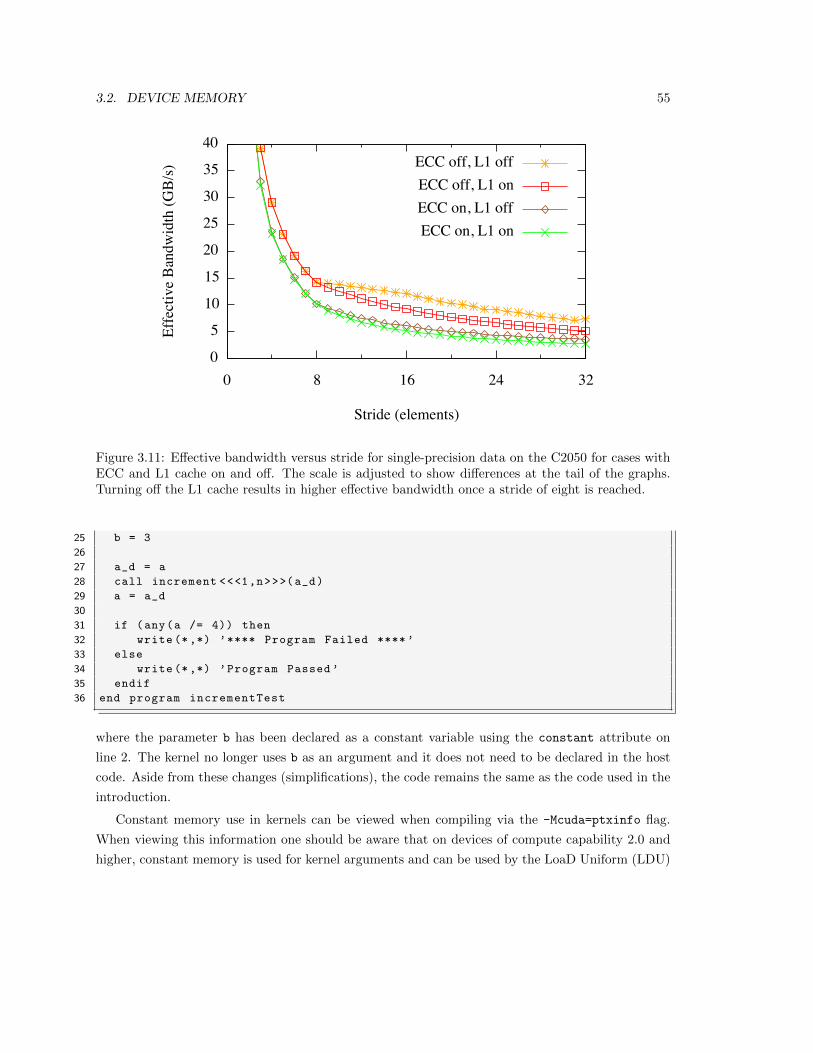
3.2. DEVICE MEMORY 55
Figure 3.11: Effective bandwidth versus stride for single-precision data on the C2050 for cases withECC and L1 cache on and off. The scale is adjusted to show differences at the tail of the graphs.Turning off the L1 cache results in higher effective bandwidth once a stride of eight is reached.
25 b = 3
26
27 a_d = a
28 call increment <<<1,n>>>(a_d)
29 a = a_d
30
31 if (any(a /= 4)) then
32 write (*,*) ’**** Program Failed ****’
33 else
34 write (*,*) ’Program Passed ’
35 endif
36 end program incrementTest
where the parameter b has been declared as a constant variable using the constant attribute on
line 2. The kernel no longer uses b as an argument and it does not need to be declared in the host
code. Aside from these changes (simplifications), the code remains the same as the code used in the
introduction.
Constant memory use in kernels can be viewed when compiling via the -Mcuda=ptxinfo flag.
When viewing this information one should be aware that on devices of compute capability 2.0 and
higher, constant memory is used for kernel arguments and can be used by the LoaD Uniform (LDU)
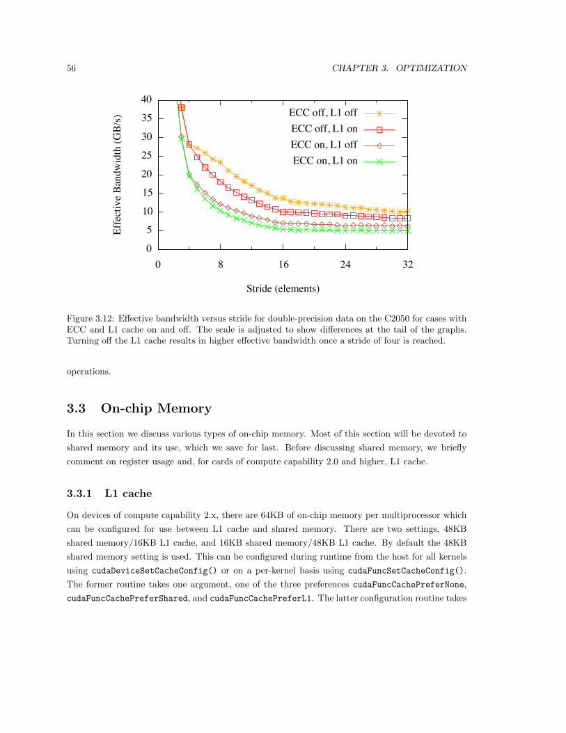
56 CHAPTER 3. OPTIMIZATION
Figure 3.12: Effective bandwidth versus stride for double-precision data on the C2050 for cases withECC and L1 cache on and off. The scale is adjusted to show differences at the tail of the graphs.Turning off the L1 cache results in higher effective bandwidth once a stride of four is reached.
operations.
3.3 On-chip Memory
In this section we discuss various types of on-chip memory. Most of this section will be devoted to
shared memory and its use, which we save for last. Before discussing shared memory, we briefly
comment on register usage and, for cards of compute capability 2.0 and higher, L1 cache.
3.3.1 L1 cache
On devices of compute capability 2.x, there are 64KB of on-chip memory per multiprocessor which
can be configured for use between L1 cache and shared memory. There are two settings, 48KB
shared memory/16KB L1 cache, and 16KB shared memory/48KB L1 cache. By default the 48KB
shared memory setting is used. This can be configured during runtime from the host for all kernels
using cudaDeviceSetCacheConfig() or on a per-kernel basis using cudaFuncSetCacheConfig().
The former routine takes one argument, one of the three preferences cudaFuncCachePreferNone,
cudaFuncCachePreferShared, and cudaFuncCachePreferL1. The latter configuration routine takes

3.3. ON-CHIP MEMORY 57
the function name for the first argument and one of three preferences as a second argument. The
compiler will honor the preferences whenever possible. The case where this is not honored is when
16KB of shared memory is requested for kernels that require more than 16KB of shared memory
per thread block.
As we have seen from the coalescing discussion for strided access of global memory, it may be
advantageous to turn L1 cache off in order to avoid 128-byte cache-line loads. This can done per
compilation unit via the flag -Mcuda=noL1.
3.3.2 Registers
Generally, accessing a register consumes zero extra clock cycles per instruction, but delays may occur
due to register read-after-write dependencies and register memory bank conflicts.
The latency of read-after-write dependencies is approximately 24 cycles, but this latency is
completely hidden on multiprocessors that have at least 192 active threads (that is, 6 warps). Note
that in the case of compute 2.0, which supports dual-issue, as many as 384 threads might be required
to completely hide latency.
The compiler and hardware thread scheduler will schedule instructions as optimally as possible
to avoid register memory bank conflicts. They achieve the best results when the number of threads
per block is a multiple of 64. Other than following this rule, an application has no direct control
over these bank conflicts.
Register pressure occurs when there are not enough registers available for a given task. Even
though each multiprocessor contains thousands of 32-bit registers, these are partitioned among
concurrent threads. The number of registers used per thread for a kernel can be obtained by using
the -Mcuda=ptxinfo option when compiling. The number of registers per thread can be limited per
compilation unit by using the -Mcuda=maxregcount:N. Limiting the number of registers per thread
can increase the number of blocks that can concurrently reside on a multiprocessor, which by itself
can result in better latency hiding. However, restricting the number of registers in this fashion will
likely increase spilling to off-chip local memory. As a result of these two opposing factors, some
experimentation is often needed to obtain the optimal situation.
3.3.3 Shared memory
Because it is on-chip, shared memory is much faster than local and global memory. In fact, uncached
shared memory latency is roughly 100x lower than global memory latency – provided there are no
bank conflicts between the threads, as detailed later in this section.
Shared memory is allocated per thread block, as all threads in the block have access to the same
shared memory. Because a thread can access shared memory that was loaded from global memory
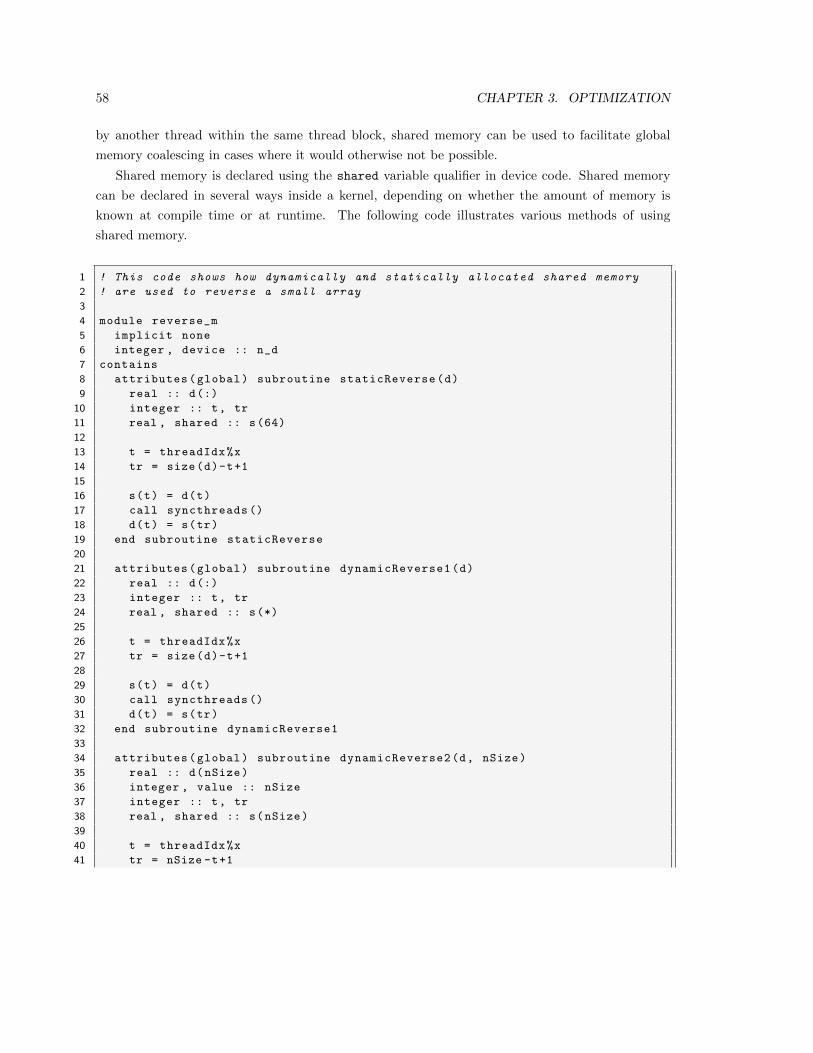
58 CHAPTER 3. OPTIMIZATION
by another thread within the same thread block, shared memory can be used to facilitate global
memory coalescing in cases where it would otherwise not be possible.
Shared memory is declared using the shared variable qualifier in device code. Shared memory
can be declared in several ways inside a kernel, depending on whether the amount of memory is
known at compile time or at runtime. The following code illustrates various methods of using
shared memory.
1 ! This code shows how dynamically and statically allocated shared memory
2 ! are used to reverse a small array
3
4 module reverse_m
5 implicit none
6 integer , device :: n_d
7 contains
8 attributes(global) subroutine staticReverse(d)
9 real :: d(:)
10 integer :: t, tr
11 real , shared :: s(64)
12
13 t = threadIdx%x
14 tr = size(d)-t+1
15
16 s(t) = d(t)
17 call syncthreads ()
18 d(t) = s(tr)
19 end subroutine staticReverse
20
21 attributes(global) subroutine dynamicReverse1(d)
22 real :: d(:)
23 integer :: t, tr
24 real , shared :: s(*)
25
26 t = threadIdx%x
27 tr = size(d)-t+1
28
29 s(t) = d(t)
30 call syncthreads ()
31 d(t) = s(tr)
32 end subroutine dynamicReverse1
33
34 attributes(global) subroutine dynamicReverse2(d, nSize)
35 real :: d(nSize)
36 integer , value :: nSize
37 integer :: t, tr
38 real , shared :: s(nSize)
39
40 t = threadIdx%x
41 tr = nSize -t+1
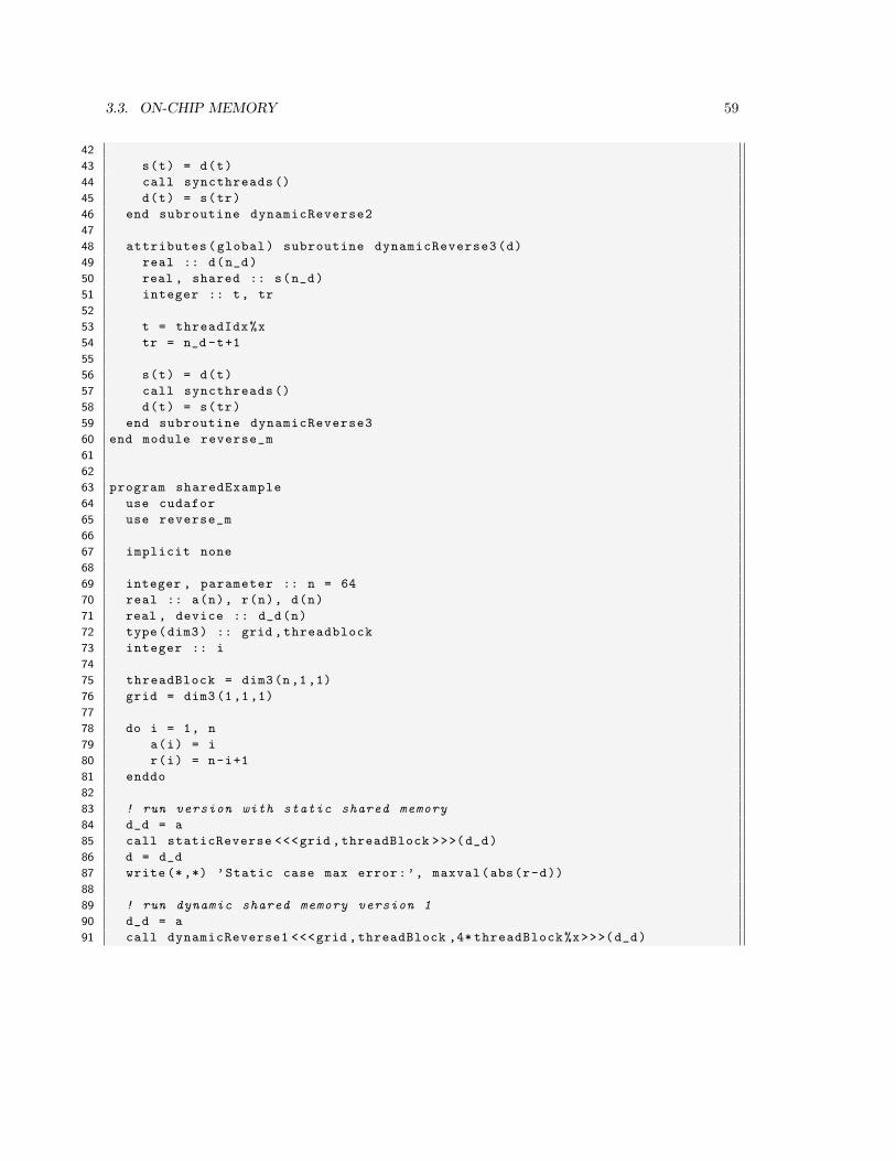
3.3. ON-CHIP MEMORY 59
42
43 s(t) = d(t)
44 call syncthreads ()
45 d(t) = s(tr)
46 end subroutine dynamicReverse2
47
48 attributes(global) subroutine dynamicReverse3(d)
49 real :: d(n_d)
50 real , shared :: s(n_d)
51 integer :: t, tr
52
53 t = threadIdx%x
54 tr = n_d -t+1
55
56 s(t) = d(t)
57 call syncthreads ()
58 d(t) = s(tr)
59 end subroutine dynamicReverse3
60 end module reverse_m
61
62
63 program sharedExample
64 use cudafor
65 use reverse_m
66
67 implicit none
68
69 integer , parameter :: n = 64
70 real :: a(n), r(n), d(n)
71 real , device :: d_d(n)
72 type(dim3) :: grid ,threadblock
73 integer :: i
74
75 threadBlock = dim3(n,1,1)
76 grid = dim3(1,1,1)
77
78 do i = 1, n
79 a(i) = i
80 r(i) = n-i+1
81 enddo
82
83 ! run version with static shared memory
84 d_d = a
85 call staticReverse <<<grid ,threadBlock >>>(d_d)
86 d = d_d
87 write (*,*) ’Static case max error:’, maxval(abs(r-d))
88
89 ! run dynamic shared memory version 1
90 d_d = a
91 call dynamicReverse1 <<<grid ,threadBlock ,4* threadBlock%x>>>(d_d)

60 CHAPTER 3. OPTIMIZATION
92 d = d_d
93 write (*,*) ’Dynamic case 1 max error:’, maxval(abs(r-d))
94
95 ! run dynamic shared memory version 2
96 d_d = a
97 call dynamicReverse2 <<<grid ,threadBlock ,4* threadBlock%x>>>(d_d ,n)
98 d = d_d
99 write (*,*) ’Dynamic case 2 max error:’, maxval(abs(r-d))
100
101 ! run dynamic shared memory version 3
102 n_d = n ! n_d declared in reverse_m
103 d_d = a
104 call dynamicReverse3 <<<grid ,threadBlock ,4* threadBlock%x>>>(d_d)
105 d = d_d
106 write (*,*) ’Dynamic case 3 max error:’, maxval(abs(r-d))
107
108 end program sharedExample
This code reverses the data in a 64-element array using shared memory. All of the kernel codes are
very similar, the main difference is how the shared memory arrays are declared, and how the kernels
are invoked. If the shared memory array size is known at compile time, as in the staticReverse
kernel, then the array is declared using that value, whether an integer parameter or literal, as is done
on line 11 with s(64). In this kernel, the two indices representing the original and reverse order are
calculated on lines 13 and 14, respectively. On line 16, the data are copied from global memory to
shared memory. The reversal is done on line 18, where both indices t and tr are used to copy data
from shared memory to global memory. Before executing line 18, where each thread accesses data in
shared memory that was written by another thread, we need to make sure all threads have completed
the loads to shared memory on line 16. This is accomplished by the barrier synchronization on line
17, syncthreads(). This barrier synchronization occurs between all threads in a thread block,
meaning that no thread can pass this line until all threads in the same thread block have reached
it. The reason shared memory is used in this example is to facilitate global memory coalescing.
Optimal global memory coalescing is achieved for both reads and writes because gobal memory is
always accessed through the index t. The reversed index tr is only used to access shared memory,
which does not have the access restrictions global memory has for optimal performance. The only
performance issue with shared memory is bank conflicts, which is discussed in the next section.
The other three kernels in this example use dynamic shared memory, where the amount of shared
memory is not known at compile time and must be specified (in bytes) when the kernel is invoked
in the optional third execution configuration parameter, as is done on lines 91, 97, and 104. The
first dynamic shared memory kernel, dynamicReverse1, declares the shared memory array on line
24 using an assumed-size array syntax. The size is implicitly determined from the third execution
configuration parameter when the kernel is launched. The remainder of the kernel code is identical
to the staticReverse kernel.
3.3. ON-CHIP MEMORY 61
As of version 11.6 of the compilers, one can use dynamic shared memory via automatic arrays,
as shown in dynamicReverse2 and dynamicReverse3. In these cases, the dimension of the dynamic
shared memory array is specified by an integer that is in scope. In dynamicReverse2, the subroutine
argument nSize is used on line 38 to declare the shared memory array size, and in dynamicReverse3
the device variable n d declared in the beginning of the module is used on line 50 to declare the
shared memory array size. Note that in both these cases the amount of dynamic memory must still
be specified in the third parameter of the execution configuration when the kernel is invoked.
Given these options for declaring dynamic shared memory, which one should be used? If one
wants to use multiple dynamic shared memory arrays, especially if they are of different types, then
one needs to use the automatic arrays as in dynamicReverse2 and dynamicReverse3. If one were
to specify multiple dynamic shared memory arrays using assumed size notation as on line 24, how
would the compiler know how to distribute the total amount of dynamic shared memory amongst
such arrays? Aside from that factor, the choice is up to the programmer, there is no performance
difference between these methods of declaration.
Shared memory bank conflicts
To achieve high memory bandwidth for concurrent accesses, shared memory is divided into equally
sized memory modules (banks) that can be accessed simultaneously. Therefore, any memory load
or store of n addresses that spans n distinct memory banks can be serviced simultaneously, yielding
an effective bandwidth that is n times as high as the bandwidth of a single bank.
However, if multiple addresses of a memory request map to the same memory bank, the accesses
are serialized. The hardware splits a memory request that has bank conflicts into as many separate
conflict-free requests as necessary, decreasing the effective bandwidth by a factor equal to the number
of separate memory requests. The one exception here is when all threads in a half warp address the
same shared memory location, resulting in a broadcast. Devices of compute capability 2.0 have the
additional ability to multicast shared memory accesses, meaning that multiple accesses to the same
location by any number of threads within a warp are served simultaneously.
To minimize bank conflicts, it is important to understand how memory addresses map to memory
banks and how to optimally schedule memory requests. Shared memory banks are organized such
that successive 32-bit words are assigned to successive banks and each bank has a bandwidth of 32
bits per clock cycle. The bandwidth of shared memory is 32 bits per bank per clock cycle.
For devices of compute capability 1.x, the warp size is 32 threads and the number of banks is
16. A shared memory request for a warp is split into one request for the first half of the warp and
one request for the second half of the warp. Note that no bank conflict occurs if only one memory
location per bank is accessed by a half warp of threads.
For devices of compute capability 2.0, the warp size is 32 threads and the number of banks is
also 32. A shared memory request for a warp is not split as with devices of compute capability 1.x,
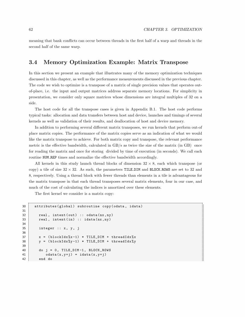
62 CHAPTER 3. OPTIMIZATION
meaning that bank conflicts can occur between threads in the first half of a warp and threads in the
second half of the same warp.
3.4 Memory Optimization Example: Matrix Transpose
In this section we present an example that illustrates many of the memory optimization techniques
discussed in this chapter, as well as the performance measurements discussed in the previous chapter.
The code we wish to optimize is a transpose of a matrix of single precision values that operates out-
of-place, i.e. the input and output matrices address separate memory locations. For simplicity in
presentation, we consider only square matrices whose dimensions are integral multiples of 32 on a
side.
The host code for all the transpose cases is given in Appendix B.1. The host code performs
typical tasks: allocation and data transfers between host and device, launches and timings of several
kernels as well as validation of their results, and deallocation of host and device memory.
In addition to performing several different matrix transposes, we run kernels that perform out-of
place matrix copies. The performance of the matrix copies serve as an indication of what we would
like the matrix transpose to achieve. For both matrix copy and transpose, the relevant performance
metric is the effective bandwidth, calculated in GB/s as twice the size of the matrix (in GB) once
for reading the matrix and once for storing divided by time of execution (in seconds). We call each
routine NUM REP times and normalize the effective bandwidth accordingly.
All kernels in this study launch thread blocks of dimension 32 × 8, each which transpose (or
copy) a tile of size 32 × 32. As such, the parameters TILE DIM and BLOCK ROWS are set to 32 and
8, respectively. Using a thread block with fewer threads than elements in a tile is advantageous for
the matrix transpose in that each thread transposes several matrix elements, four in our case, and
much of the cost of calculating the indices is amortized over these elements.
The first kernel we consider is a matrix copy:
30 attributes(global) subroutine copy(odata , idata)
31
32 real , intent(out) :: odata(nx,ny)
33 real , intent(in) :: idata(nx,ny)
34
35 integer :: x, y, j
36
37 x = (blockIdx%x-1) * TILE_DIM + threadIdx%x
38 y = (blockIdx%y-1) * TILE_DIM + threadIdx%y
39
40 do j = 0, TILE_DIM -1, BLOCK_ROWS
41 odata(x,y+j) = idata(x,y+j)
42 end do
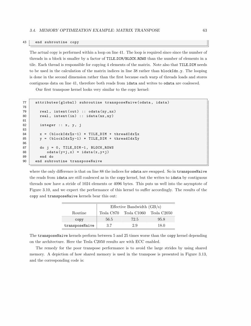
3.4. MEMORY OPTIMIZATION EXAMPLE: MATRIX TRANSPOSE 63
43 end subroutine copy
The actual copy is performed within a loop on line 41. The loop is required since since the number of
threads in a block is smaller by a factor of TILE DIM/BLOCK ROWS than the number of elements in a
tile. Each thread is responsible for copying 4 elements of the matrix. Note also that TILE DIM needs
to be used in the calculation of the matrix indices in line 38 rather than blockIdx.y. The looping
is done in the second dimension rather than the first because each warp of threads loads and stores
contiguous data on line 41, therefore both reads from idata and writes to odata are coalesced.
Our first transpose kernel looks very similar to the copy kernel:
77 attributes(global) subroutine transposeNaive(odata , idata)
78
79 real , intent(out) :: odata(ny,nx)
80 real , intent(in) :: idata(nx,ny)
81
82 integer :: x, y, j
83
84 x = (blockIdx%x-1) * TILE_DIM + threadIdx%x
85 y = (blockIdx%y-1) * TILE_DIM + threadIdx%y
86
87 do j = 0, TILE_DIM -1, BLOCK_ROWS
88 odata(y+j,x) = idata(x,y+j)
89 end do
90 end subroutine transposeNaive
where the only difference is that on line 88 the indices for odata are swapped. So in transposeNaive
the reads from idata are still coalesced as in the copy kernel, but the writes to idata by contiguous
threads now have a stride of 1024 elements or 4096 bytes. This puts us well into the asymptote of
Figure 3.10, and we expect the performance of this kernel to suffer accordingly. The results of the
copy and transposeNaive kernels bear this out:
Effective Bandwidth (GB/s)
Routine Tesla C870 Tesla C1060 Tesla C2050
copy 56.5 72.5 95.8
transposeNaive 3.7 2.9 18.0
The transposeNaive kernels perform between 5 and 25 times worse than the copy kernel depending
on the architecture. Here the Tesla C2050 results are with ECC enabled.
The remedy for the poor transpose performance is to avoid the large strides by using shared
memory. A depiction of how shared memory is used in the transpose is presented in Figure 3.13,
and the corresponding code is:
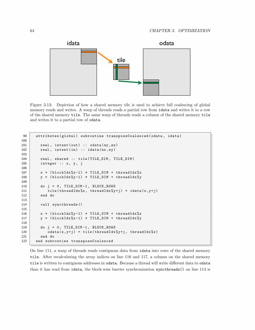
64 CHAPTER 3. OPTIMIZATION
idata odata
tile
Figure 3.13: Depiction of how a shared memory tile is used to achieve full coalescing of globalmemory reads and writes. A warp of threads reads a partial row from idata and writes it to a rowof the shared memory tile. The same warp of threads reads a column of the shared memory tile
and writes it to a partial row of odata.
99 attributes(global) subroutine transposeCoalesced(odata , idata)
100
101 real , intent(out) :: odata(ny,nx)
102 real , intent(in) :: idata(nx,ny)
103
104 real , shared :: tile(TILE_DIM , TILE_DIM)
105 integer :: x, y, j
106
107 x = (blockIdx%x-1) * TILE_DIM + threadIdx%x
108 y = (blockIdx%y-1) * TILE_DIM + threadIdx%y
109
110 do j = 0, TILE_DIM -1, BLOCK_ROWS
111 tile(threadIdx%x, threadIdx%y+j) = idata(x,y+j)
112 end do
113
114 call syncthreads ()
115
116 x = (blockIdx%y-1) * TILE_DIM + threadIdx%x
117 y = (blockIdx%x-1) * TILE_DIM + threadIdx%y
118
119 do j = 0, TILE_DIM -1, BLOCK_ROWS
120 odata(x,y+j) = tile(threadIdx%y+j, threadIdx%x)
121 end do
122 end subroutine transposeCoalesced
On line 111, a warp of threads reads contiguous data from idata into rows of the shared memory
tile. After recalculating the array indices on line 116 and 117, a column on the shared memory
tile is written to contiguous addresses in odata. Because a thread will write different data to odata
than it has read from idata, the block-wise barrier synchronization syncthreads() on line 114 is
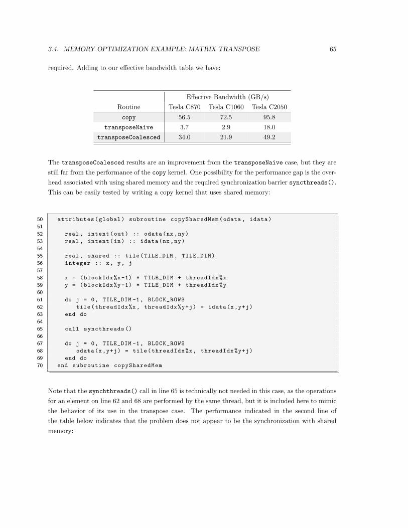
3.4. MEMORY OPTIMIZATION EXAMPLE: MATRIX TRANSPOSE 65
required. Adding to our effective bandwidth table we have:
Effective Bandwidth (GB/s)
Routine Tesla C870 Tesla C1060 Tesla C2050
copy 56.5 72.5 95.8
transposeNaive 3.7 2.9 18.0
transposeCoalesced 34.0 21.9 49.2
The transposeCoalesced results are an improvement from the transposeNaive case, but they are
still far from the performance of the copy kernel. One possibility for the performance gap is the over-
head associated with using shared memory and the required synchronization barrier syncthreads().
This can be easily tested by writing a copy kernel that uses shared memory:
50 attributes(global) subroutine copySharedMem(odata , idata)
51
52 real , intent(out) :: odata(nx,ny)
53 real , intent(in) :: idata(nx,ny)
54
55 real , shared :: tile(TILE_DIM , TILE_DIM)
56 integer :: x, y, j
57
58 x = (blockIdx%x-1) * TILE_DIM + threadIdx%x
59 y = (blockIdx%y-1) * TILE_DIM + threadIdx%y
60
61 do j = 0, TILE_DIM -1, BLOCK_ROWS
62 tile(threadIdx%x, threadIdx%y+j) = idata(x,y+j)
63 end do
64
65 call syncthreads ()
66
67 do j = 0, TILE_DIM -1, BLOCK_ROWS
68 odata(x,y+j) = tile(threadIdx%x, threadIdx%y+j)
69 end do
70 end subroutine copySharedMem
Note that the synchthreads() call in line 65 is technically not needed in this case, as the operations
for an element on line 62 and 68 are performed by the same thread, but it is included here to mimic
the behavior of its use in the transpose case. The performance indicated in the second line of
the table below indicates that the problem does not appear to be the synchronization with shared
memory:
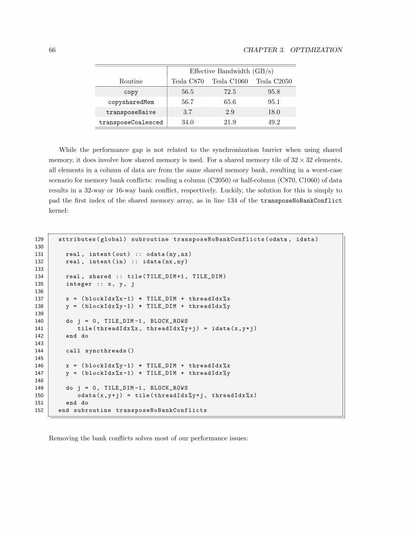
66 CHAPTER 3. OPTIMIZATION
Effective Bandwidth (GB/s)
Routine Tesla C870 Tesla C1060 Tesla C2050
copy 56.5 72.5 95.8
copysharedMem 56.7 65.6 95.1
transposeNaive 3.7 2.9 18.0
transposeCoalesced 34.0 21.9 49.2
While the performance gap is not related to the synchronization barrier when using shared
memory, it does involve how shared memory is used. For a shared memory tile of 32× 32 elements,
all elements in a column of data are from the same shared memory bank, resulting in a worst-case
scenario for memory bank conflicts: reading a column (C2050) or half-column (C870, C1060) of data
results in a 32-way or 16-way bank conflict, respectively. Luckily, the solution for this is simply to
pad the first index of the shared memory array, as in line 134 of the transposeNoBankConflict
kernel:
129 attributes(global) subroutine transposeNoBankConflicts(odata , idata)
130
131 real , intent(out) :: odata(ny,nx)
132 real , intent(in) :: idata(nx,ny)
133
134 real , shared :: tile(TILE_DIM+1, TILE_DIM)
135 integer :: x, y, j
136
137 x = (blockIdx%x-1) * TILE_DIM + threadIdx%x
138 y = (blockIdx%y-1) * TILE_DIM + threadIdx%y
139
140 do j = 0, TILE_DIM -1, BLOCK_ROWS
141 tile(threadIdx%x, threadIdx%y+j) = idata(x,y+j)
142 end do
143
144 call syncthreads ()
145
146 x = (blockIdx%y-1) * TILE_DIM + threadIdx%x
147 y = (blockIdx%x-1) * TILE_DIM + threadIdx%y
148
149 do j = 0, TILE_DIM -1, BLOCK_ROWS
150 odata(x,y+j) = tile(threadIdx%y+j, threadIdx%x)
151 end do
152 end subroutine transposeNoBankConflicts
Removing the bank conflicts solves most of our performance issues:
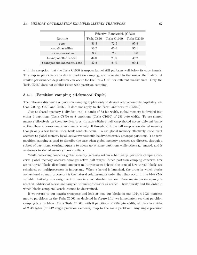
3.4. MEMORY OPTIMIZATION EXAMPLE: MATRIX TRANSPOSE 67
Effective Bandwidth (GB/s)
Routine Tesla C870 Tesla C1060 Tesla C2050
copy 56.5 72.5 95.8
copySharedMem 56.7 65.6 95.1
transposeNaive 3.7 2.9 18.0
transposeCoalesced 34.0 21.9 49.2
transposeNoBankConflicts 42.2 21.9 90.4
with the exception that the Tesla C1060 transpose kernel still performs well below its copy kernels.
This gap in performance is due to partition camping, and is related to the size of the matrix. A
similar performance degradation can occur for the Tesla C870 for different matrix sizes. Only the
Tesla C2050 does not exhibit issues with partition camping.
3.4.1 Partition camping (Advanced Topic)
The following discussion of partition camping applies only to devices with a compute capability less
than 2.0, eg. C870 and C1060. It does not apply to the Fermi architecture (C2050).
Just as shared memory is divided into 16 banks of 32-bit width, global memory is divided into
either 6 partitions (Tesla C870) or 8 partitions (Tesla C1060) of 256-byte width. To use shared
memory effectively on these architectures, threads within a half warp should access different banks
so that these accesses can occur simultaneously. If threads within a half warp access shared memory
though only a few banks, then bank conflicts occur. To use global memory effectively, concurrent
accesses to global memory by all active warps should be divided evenly amongst partitions. The term
partition camping is used to describe the case when global memory accesses are directed through a
subset of partitions, causing requests to queue up at some partitions while others go unused, and is
analogous to shared memory bank conflicts.
While coalescing concerns global memory accesses within a half warp, partition camping con-
cerns global memory accesses amongst active half warps. Since partition camping concerns how
active thread blocks distributed amongst multiprocessors behave, the issue of how thread blocks are
scheduled on multiprocessors is important. When a kernel is launched, the order in which blocks
are assigned to multiprocessors is the natural column-major order that they occur in the blockIdx
variable. Initially this assignment occurs in a round-robin fashion. Once maximum occupancy is
reached, additional blocks are assigned to multiprocessors as needed – how quickly and the order in
which blocks complete kernels cannot be determined.
If we return to our matrix transpose and look at how our blocks in our 1024 × 1024 matrices
map to partitions on the Tesla C1060, as depicted in Figure 3.14, we immediately see that partition
camping is a problem. On a Tesla C1060, with 8 partitions of 256-byte width, all data in strides
of 2048 bytes (or 512 single precision elements) map to the same partition. Any single precision
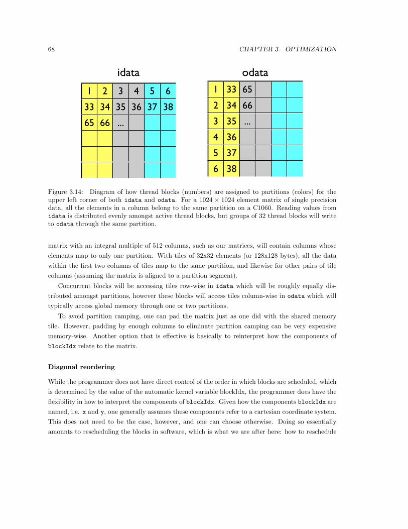
68 CHAPTER 3. OPTIMIZATION
1 2 3 4 5 6
33 34 35 36 37 38
65 66 ...
1 33 65
2 34 66
3 35 ...
4 36
5 37
6 38
idata odata
Figure 3.14: Diagram of how thread blocks (numbers) are assigned to partitions (colors) for theupper left corner of both idata and odata. For a 1024 × 1024 element matrix of single precisiondata, all the elements in a column belong to the same partition on a C1060. Reading values fromidata is distributed evenly amongst active thread blocks, but groups of 32 thread blocks will writeto odata through the same partition.
matrix with an integral multiple of 512 columns, such as our matrices, will contain columns whose
elements map to only one partition. With tiles of 32x32 elements (or 128x128 bytes), all the data
within the first two columns of tiles map to the same partition, and likewise for other pairs of tile
columns (assuming the matrix is aligned to a partition segment).
Concurrent blocks will be accessing tiles row-wise in idata which will be roughly equally dis-
tributed amongst partitions, however these blocks will access tiles column-wise in odata which will
typically access global memory through one or two partitions.
To avoid partition camping, one can pad the matrix just as one did with the shared memory
tile. However, padding by enough columns to eliminate partition camping can be very expensive
memory-wise. Another option that is effective is basically to reinterpret how the components of
blockIdx relate to the matrix.
Diagonal reordering
While the programmer does not have direct control of the order in which blocks are scheduled, which
is determined by the value of the automatic kernel variable blockIdx, the programmer does have the
flexibility in how to interpret the components of blockIdx. Given how the components blockIdx are
named, i.e. x and y, one generally assumes these components refer to a cartesian coordinate system.
This does not need to be the case, however, and one can choose otherwise. Doing so essentially
amounts to rescheduling the blocks in software, which is what we are after here: how to reschedule
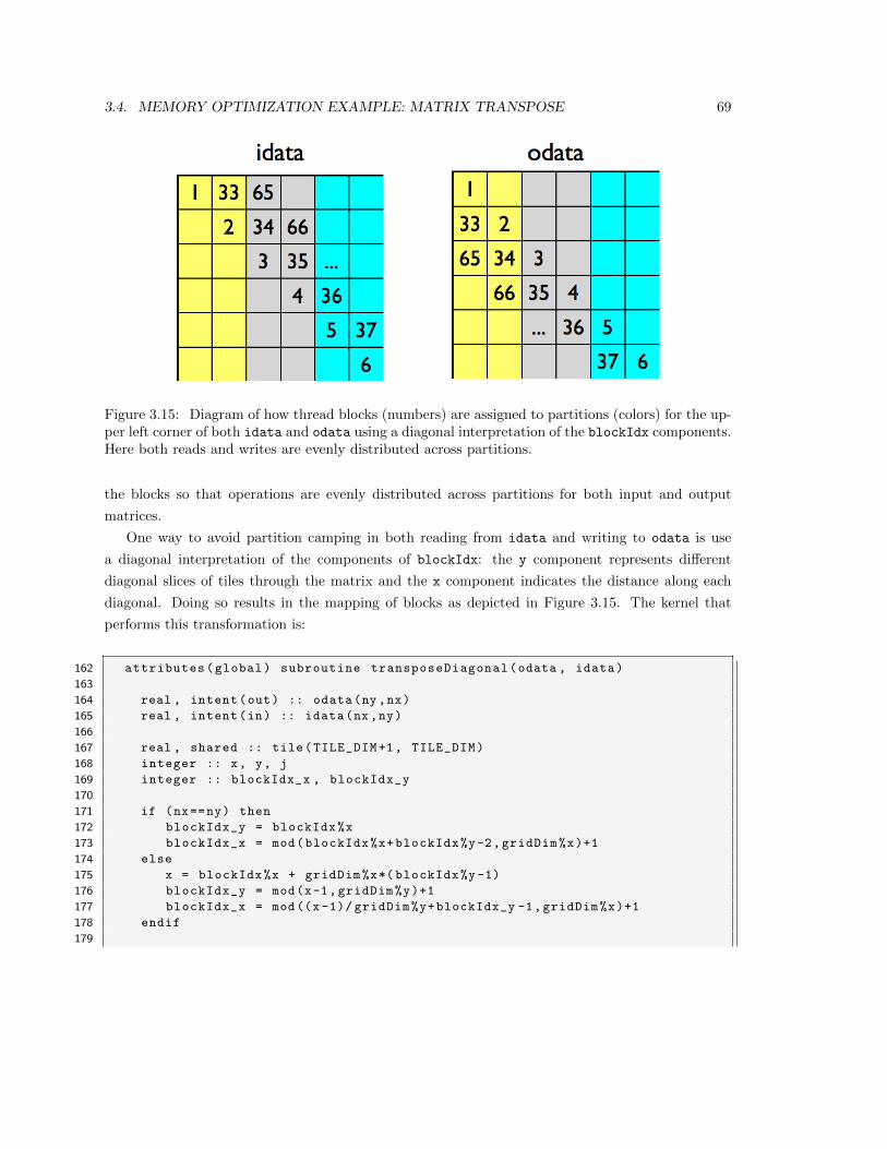
3.4. MEMORY OPTIMIZATION EXAMPLE: MATRIX TRANSPOSE 69
Figure 3.15: Diagram of how thread blocks (numbers) are assigned to partitions (colors) for the up-per left corner of both idata and odata using a diagonal interpretation of the blockIdx components.Here both reads and writes are evenly distributed across partitions.
the blocks so that operations are evenly distributed across partitions for both input and output
matrices.
One way to avoid partition camping in both reading from idata and writing to odata is use
a diagonal interpretation of the components of blockIdx: the y component represents different
diagonal slices of tiles through the matrix and the x component indicates the distance along each
diagonal. Doing so results in the mapping of blocks as depicted in Figure 3.15. The kernel that
performs this transformation is:
162 attributes(global) subroutine transposeDiagonal(odata , idata)
163
164 real , intent(out) :: odata(ny,nx)
165 real , intent(in) :: idata(nx,ny)
166
167 real , shared :: tile(TILE_DIM+1, TILE_DIM)
168 integer :: x, y, j
169 integer :: blockIdx_x , blockIdx_y
170
171 if (nx==ny) then
172 blockIdx_y = blockIdx%x
173 blockIdx_x = mod(blockIdx%x+blockIdx%y-2,gridDim%x)+1
174 else
175 x = blockIdx%x + gridDim%x*( blockIdx%y-1)
176 blockIdx_y = mod(x-1,gridDim%y)+1
177 blockIdx_x = mod((x-1)/ gridDim%y+blockIdx_y -1,gridDim%x)+1
178 endif
179
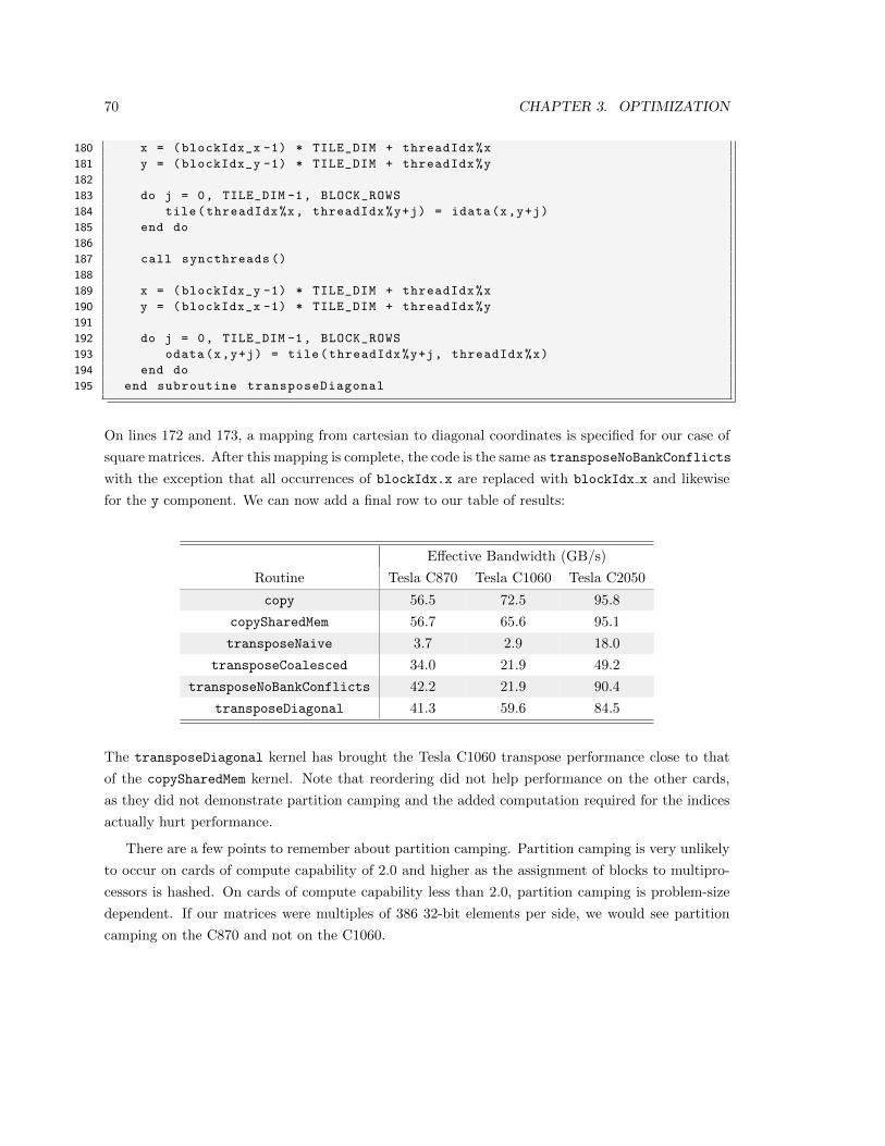
70 CHAPTER 3. OPTIMIZATION
180 x = (blockIdx_x -1) * TILE_DIM + threadIdx%x
181 y = (blockIdx_y -1) * TILE_DIM + threadIdx%y
182
183 do j = 0, TILE_DIM -1, BLOCK_ROWS
184 tile(threadIdx%x, threadIdx%y+j) = idata(x,y+j)
185 end do
186
187 call syncthreads ()
188
189 x = (blockIdx_y -1) * TILE_DIM + threadIdx%x
190 y = (blockIdx_x -1) * TILE_DIM + threadIdx%y
191
192 do j = 0, TILE_DIM -1, BLOCK_ROWS
193 odata(x,y+j) = tile(threadIdx%y+j, threadIdx%x)
194 end do
195 end subroutine transposeDiagonal
On lines 172 and 173, a mapping from cartesian to diagonal coordinates is specified for our case of
square matrices. After this mapping is complete, the code is the same as transposeNoBankConflicts
with the exception that all occurrences of blockIdx.x are replaced with blockIdx x and likewise
for the y component. We can now add a final row to our table of results:
Effective Bandwidth (GB/s)
Routine Tesla C870 Tesla C1060 Tesla C2050
copy 56.5 72.5 95.8
copySharedMem 56.7 65.6 95.1
transposeNaive 3.7 2.9 18.0
transposeCoalesced 34.0 21.9 49.2
transposeNoBankConflicts 42.2 21.9 90.4
transposeDiagonal 41.3 59.6 84.5
The transposeDiagonal kernel has brought the Tesla C1060 transpose performance close to that
of the copySharedMem kernel. Note that reordering did not help performance on the other cards,
as they did not demonstrate partition camping and the added computation required for the indices
actually hurt performance.
There are a few points to remember about partition camping. Partition camping is very unlikely
to occur on cards of compute capability of 2.0 and higher as the assignment of blocks to multipro-
cessors is hashed. On cards of compute capability less than 2.0, partition camping is problem-size
dependent. If our matrices were multiples of 386 32-bit elements per side, we would see partition
camping on the C870 and not on the C1060.
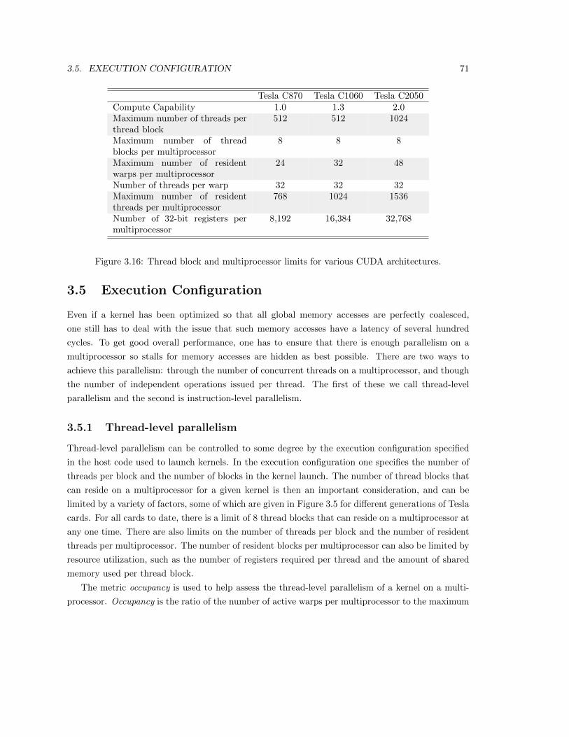
3.5. EXECUTION CONFIGURATION 71
Tesla C870 Tesla C1060 Tesla C2050Compute Capability 1.0 1.3 2.0Maximum number of threads perthread block
512 512 1024
Maximum number of threadblocks per multiprocessor
8 8 8
Maximum number of residentwarps per multiprocessor
24 32 48
Number of threads per warp 32 32 32Maximum number of residentthreads per multiprocessor
768 1024 1536
Number of 32-bit registers permultiprocessor
8,192 16,384 32,768
Figure 3.16: Thread block and multiprocessor limits for various CUDA architectures.
3.5 Execution Configuration
Even if a kernel has been optimized so that all global memory accesses are perfectly coalesced,
one still has to deal with the issue that such memory accesses have a latency of several hundred
cycles. To get good overall performance, one has to ensure that there is enough parallelism on a
multiprocessor so stalls for memory accesses are hidden as best possible. There are two ways to
achieve this parallelism: through the number of concurrent threads on a multiprocessor, and though
the number of independent operations issued per thread. The first of these we call thread-level
parallelism and the second is instruction-level parallelism.
3.5.1 Thread-level parallelism
Thread-level parallelism can be controlled to some degree by the execution configuration specified
in the host code used to launch kernels. In the execution configuration one specifies the number of
threads per block and the number of blocks in the kernel launch. The number of thread blocks that
can reside on a multiprocessor for a given kernel is then an important consideration, and can be
limited by a variety of factors, some of which are given in Figure 3.5 for different generations of Tesla
cards. For all cards to date, there is a limit of 8 thread blocks that can reside on a multiprocessor at
any one time. There are also limits on the number of threads per block and the number of resident
threads per multiprocessor. The number of resident blocks per multiprocessor can also be limited by
resource utilization, such as the number of registers required per thread and the amount of shared
memory used per thread block.
The metric occupancy is used to help assess the thread-level parallelism of a kernel on a multi-
processor. Occupancy is the ratio of the number of active warps per multiprocessor to the maximum
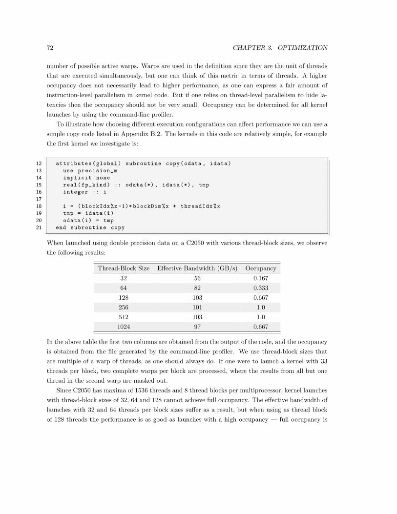
72 CHAPTER 3. OPTIMIZATION
number of possible active warps. Warps are used in the definition since they are the unit of threads
that are executed simultaneously, but one can think of this metric in terms of threads. A higher
occupancy does not necessarily lead to higher performance, as one can express a fair amount of
instruction-level parallelism in kernel code. But if one relies on thread-level parallelism to hide la-
tencies then the occupancy should not be very small. Occupancy can be determined for all kernel
launches by using the command-line profiler.
To illustrate how choosing different execution configurations can affect performance we can use a
simple copy code listed in Appendix B.2. The kernels in this code are relatively simple, for example
the first kernel we investigate is:
12 attributes(global) subroutine copy(odata , idata)
13 use precision_m
14 implicit none
15 real(fp_kind) :: odata (*), idata (*), tmp
16 integer :: i
17
18 i = (blockIdx%x-1)* blockDim%x + threadIdx%x
19 tmp = idata(i)
20 odata(i) = tmp
21 end subroutine copy
When launched using double precision data on a C2050 with various thread-block sizes, we observe
the following results:
Thread-Block Size Effective Bandwidth (GB/s) Occupancy
32 56 0.167
64 82 0.333
128 103 0.667
256 101 1.0
512 103 1.0
1024 97 0.667
In the above table the first two columns are obtained from the output of the code, and the occupancy
is obtained from the file generated by the command-line profiler. We use thread-block sizes that
are multiple of a warp of threads, as one should always do. If one were to launch a kernel with 33
threads per block, two complete warps per block are processed, where the results from all but one
thread in the second warp are masked out.
Since C2050 has maxima of 1536 threads and 8 thread blocks per multiprocessor, kernel launches
with thread-block sizes of 32, 64 and 128 cannot achieve full occupancy. The effective bandwidth of
launches with 32 and 64 threads per block sizes suffer as a result, but when using as thread block
of 128 threads the performance is as good as launches with a high occupancy — full occupancy is

3.5. EXECUTION CONFIGURATION 73
not needed to achieve good performance. Also notice that more threads per block does not mean
higher occupancy. There are granularity issues that must be taken into account. An occupancy of
two thirds is the best one can achieve when using 1024 threads per block, as only a single block of
this size can reside on a multiprocessor at any one time.
Shared memory
Shared memory can be helpful in several situations, such as helping to coalesce or eliminate redun-
dant access to global memory. However, it also can act as a constraint on occupancy. Our example
code above does not use shared memory in the kernel, however one can determine the sensitivity
of performance to occupancy by changing the amount of dynamically allocated shared memory, as
specified in the third parameter of the execution configuration. By simply increasing this parameter
(without modifying the kernel), it is possible to effectively reduce the occupancy of the kernel and
measure its effect on performance. For example, if we launch the same copy kernel using:
121 call copy <<<grid , threadBlock , 0.9* smBytes >>>(b_d , a_d)
where smBytes is the size of shared memory per multiprocessor in bytes, then we force there to be
only one concurrent thread block per multiprocessor. Doing so yields the following results:
Thread-Block Size Effective Bandwidth (GB/s) Occupancy
32 8 0.021
64 15 0.042
128 29 0.083
256 51 0.167
512 75 0.333
1024 97 0.667
The occupancy numbers indicate that indeed only one thread block resides at any one time on
a multiprocessor, and the performance degrades as one would expect. This exercise prompts the
question: what can be done in more complicated kernels where either register or shared memory use
limits the occupancy? Does one have to put up with poor performance in such cases? The answer
is no, if one uses instruction-level parallelism.
3.5.2 Instruction-level parallelism
We have already seen an example of instruction-level parallelism in this book. In the transpose
example of Section 3.4, a shared-memory tile of 32 × 32 was used in most of the kernels. But
because the maximum number of threads per block is 512 on certain devices, it is not possible to
launch a kernel with 32 × 32 threads per block. Instead, one has to use a thread block with fewer
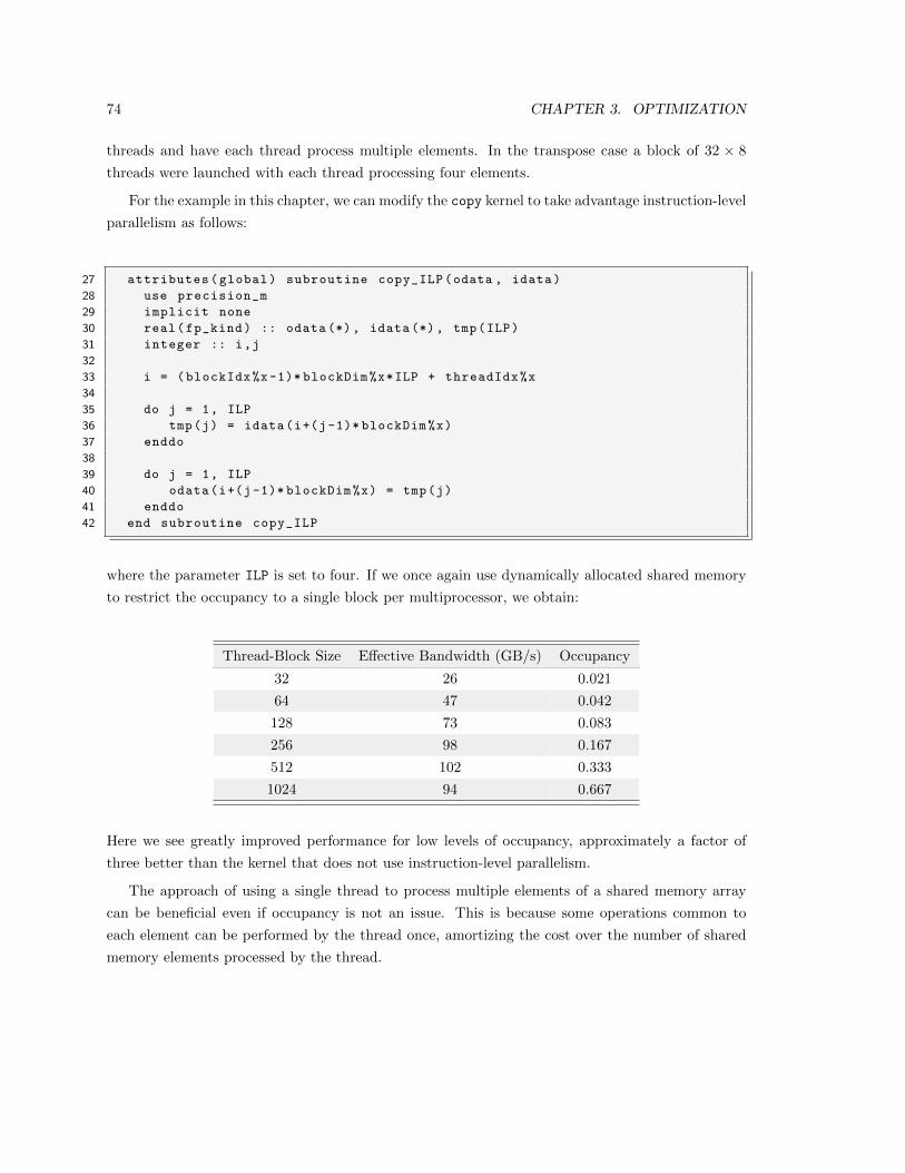
74 CHAPTER 3. OPTIMIZATION
threads and have each thread process multiple elements. In the transpose case a block of 32 × 8
threads were launched with each thread processing four elements.
For the example in this chapter, we can modify the copy kernel to take advantage instruction-level
parallelism as follows:
27 attributes(global) subroutine copy_ILP(odata , idata)
28 use precision_m
29 implicit none
30 real(fp_kind) :: odata (*), idata (*), tmp(ILP)
31 integer :: i,j
32
33 i = (blockIdx%x-1)* blockDim%x*ILP + threadIdx%x
34
35 do j = 1, ILP
36 tmp(j) = idata(i+(j-1)* blockDim%x)
37 enddo
38
39 do j = 1, ILP
40 odata(i+(j-1)* blockDim%x) = tmp(j)
41 enddo
42 end subroutine copy_ILP
where the parameter ILP is set to four. If we once again use dynamically allocated shared memory
to restrict the occupancy to a single block per multiprocessor, we obtain:
Thread-Block Size Effective Bandwidth (GB/s) Occupancy
32 26 0.021
64 47 0.042
128 73 0.083
256 98 0.167
512 102 0.333
1024 94 0.667
Here we see greatly improved performance for low levels of occupancy, approximately a factor of
three better than the kernel that does not use instruction-level parallelism.
The approach of using a single thread to process multiple elements of a shared memory array
can be beneficial even if occupancy is not an issue. This is because some operations common to
each element can be performed by the thread once, amortizing the cost over the number of shared
memory elements processed by the thread.
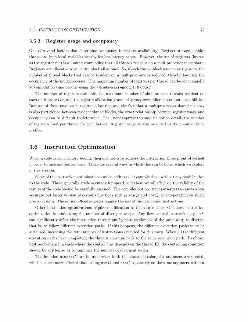
3.6. INSTRUCTION OPTIMIZATION 75
3.5.3 Register usage and occupancy
One of several factors that determine occupancy is register availability. Register storage enables
threads to keep local variables nearby for low-latency access. However, the set of registers (known
as the register file) is a limited commodity that all threads resident on a multiprocessor must share.
Registers are allocated to an entire block all at once. So, if each thread block uses many registers, the
number of thread blocks that can be resident on a multiprocessor is reduced, thereby lowering the
occupancy of the multiprocessor. The maximum number of registers per thread can be set manually
at compilation time per-file using the -Mcuda=maxregcount:N option.
The number of registers available, the maximum number of simultaneous threads resident on
each multiprocessor, and the register allocation granularity vary over different compute capabilities.
Because of these nuances in register allocation and the fact that a multiprocessors shared memory
is also partitioned between resident thread blocks, the exact relationship between register usage and
occupancy can be difficult to determine. The -Mcuda=ptxinfo compiler option details the number
of registers used per thread for each kernel. Register usage is also provided in the command-line
profiler.
3.6 Instruction Optimization
When a code is not memory bound, then one needs to address the instruction throughput of kernels
in order to increase performance. There are several ways in which this can be done, which we explore
in this section.
Some of the instruction optimizations can be addressed at compile time, without any modification
to the code. These generally trade accuracy for speed, and their overall effect on the validity of the
results of the code should be carefully assessed. The compiler option -Mcuda=fastmath causes a less
accurate but faster version of certains functions such as sin() and cos() when operating on single
precision data. The option -Mcuda=nofma toggles the use of fused mul-add instructions.
Other instruction optimizations require modification to the source code. One such instruction
optimization is minimizing the number of divergent warps. Any flow control instruction, eg. if,
can significantly affect the instruction throughput by causing threads of the same warp to diverge;
that is, to follow different execution paths. If this happens, the different execution paths must be
serialized, increasing the total number of instructions executed for this warp. When all the different
execution paths have completed, the threads converge back to the same execution path. To obtain
best performance in cases where the control flow depends on the thread ID, the controlling condition
should be written so as to minimize the number of divergent warps.
The function sincos() can be used when both the sine and cosine of a argument are needed,
which is much more efficient than calling sin() and cos() separately on the same argument without

76 CHAPTER 3. OPTIMIZATION
any loss in precision.

Part II
Case Studies
77


Chapter 4
Monte Carlo Method
A book on high performance and parallel computing is not complete without an example that shows
how to compute π. Instead of using the classic example of numerical integration of the function∫ 1
04
1+x2 dx, we are going to use a Monte Carlo method to compute π.
Figure 4.1: Monte Carlo method: π is
computed as the ratio between the red
points and the total number of points
Calculating π using a Monte Carlo method is quite sim-
ple. In a unit square we generate a sequence of N points,
(xi, yi) with i = 1, . . . , N , where each component is a ran-
dom number with uniform distribution. We then count
the number of points, M, that are inside the unit circle
(i.e. satisfy the relationship x2i + y2
i <= 1). The ratio of
M to N will give us an estimate of π/4, which is the ratio
of the area of a quarter of the unit circle, π/4, to the area
of the unit square, 1. The method is inherently parallel,
as every point can be evaluated independently, so we are
expecting good performance and scalability on the GPU.
The accuracy of the ratio depends on the number of
points used. The convergence to the real value is very
slow: simple Monte Carlo methods like the one just pre-
sented have a convergence O(1/√N). There are algorith-
mic improvements like importance sampling and the use of
low-discrepancy sequences (quasi-Monte Carlo methods)
to improve the convergence speed, but these are beyond the scope of this book.
To write a CUDA Fortran code to solve this problem, the first issue we face is how to generate the
random numbers on the GPU. Parallel random number generation is a fascinating subject, but we
are going to take a shortcut and use CURAND, the library for random number generation provided
79
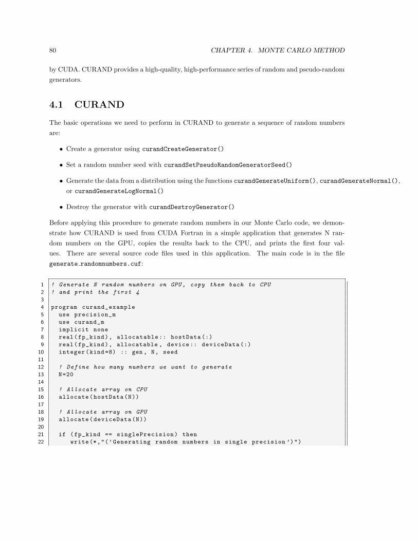
80 CHAPTER 4. MONTE CARLO METHOD
by CUDA. CURAND provides a high-quality, high-performance series of random and pseudo-random
generators.
4.1 CURAND
The basic operations we need to perform in CURAND to generate a sequence of random numbers
are:
• Create a generator using curandCreateGenerator()
• Set a random number seed with curandSetPseudoRandomGeneratorSeed()
• Generate the data from a distribution using the functions curandGenerateUniform(), curandGenerateNormal(),
or curandGenerateLogNormal()
• Destroy the generator with curandDestroyGenerator()
Before applying this procedure to generate random numbers in our Monte Carlo code, we demon-
strate how CURAND is used from CUDA Fortran in a simple application that generates N ran-
dom numbers on the GPU, copies the results back to the CPU, and prints the first four val-
ues. There are several source code files used in this application. The main code is in the file
generate randomnumbers.cuf:
1 ! Generate N random numbers on GPU , copy them back to CPU
2 ! and print the first 4
3
4 program curand_example
5 use precision_m
6 use curand_m
7 implicit none
8 real(fp_kind), allocatable :: hostData (:)
9 real(fp_kind), allocatable , device :: deviceData (:)
10 integer(kind =8) :: gen , N, seed
11
12 ! Define how many numbers we want to generate
13 N=20
14
15 ! Allocate array on CPU
16 allocate(hostData(N))
17
18 ! Allocate array on GPU
19 allocate(deviceData(N))
20
21 if (fp_kind == singlePrecision) then
22 write(*,"(’Generating random numbers in single precision ’)")
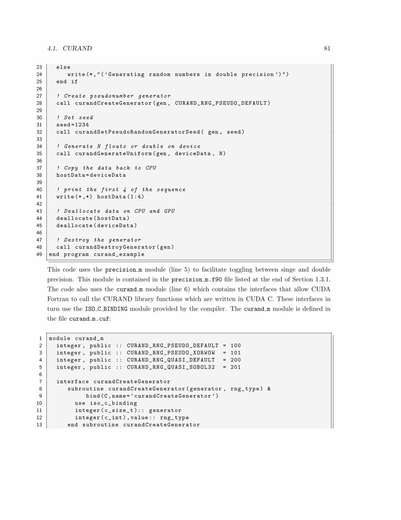
4.1. CURAND 81
23 else
24 write(*,"(’Generating random numbers in double precision ’)")
25 end if
26
27 ! Create pseudonumber generator
28 call curandCreateGenerator(gen , CURAND_RNG_PSEUDO_DEFAULT)
29
30 ! Set seed
31 seed =1234
32 call curandSetPseudoRandomGeneratorSeed( gen , seed)
33
34 ! Generate N floats or double on device
35 call curandGenerateUniform(gen , deviceData , N)
36
37 ! Copy the data back to CPU
38 hostData=deviceData
39
40 ! print the first 4 of the sequence
41 write (*,*) hostData (1:4)
42
43 ! Deallocate data on CPU and GPU
44 deallocate(hostData)
45 deallocate(deviceData)
46
47 ! Destroy the generator
48 call curandDestroyGenerator(gen)
49 end program curand_example
This code uses the precision m module (line 5) to facilitate toggling between singe and double
precision. This module is contained in the precision m.f90 file listed at the end of Section 1.3.1.
The code also uses the curand m module (line 6) which contains the interfaces that allow CUDA
Fortran to call the CURAND library functions which are written in CUDA C. These interfaces in
turn use the ISO C BINDING module provided by the compiler. The curand m module is defined in
the file curand m.cuf:
1 module curand_m
2 integer , public :: CURAND_RNG_PSEUDO_DEFAULT = 100
3 integer , public :: CURAND_RNG_PSEUDO_XORWOW = 101
4 integer , public :: CURAND_RNG_QUASI_DEFAULT = 200
5 integer , public :: CURAND_RNG_QUASI_SOBOL32 = 201
6
7 interface curandCreateGenerator
8 subroutine curandCreateGenerator(generator , rng_type) &
9 bind(C,name=’curandCreateGenerator ’)
10 use iso_c_binding
11 integer(c_size_t ):: generator
12 integer(c_int),value:: rng_type
13 end subroutine curandCreateGenerator
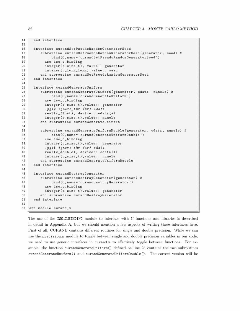
82 CHAPTER 4. MONTE CARLO METHOD
14 end interface
15
16 interface curandSetPseudoRandomGeneratorSeed
17 subroutine curandSetPseudoRandomGeneratorSeed(generator , seed) &
18 bind(C,name=’curandSetPseudoRandomGeneratorSeed ’)
19 use iso_c_binding
20 integer(c_size_t), value:: generator
21 integer(c_long_long),value:: seed
22 end subroutine curandSetPseudoRandomGeneratorSeed
23 end interface
24
25 interface curandGenerateUniform
26 subroutine curandGenerateUniform(generator , odata , numele) &
27 bind(C,name=’curandGenerateUniform ’)
28 use iso_c_binding
29 integer(c_size_t),value:: generator
30 !pgi$ ignore_tkr (tr) odata
31 real(c_float), device :: odata (*)
32 integer(c_size_t),value:: numele
33 end subroutine curandGenerateUniform
34
35 subroutine curandGenerateUniformDouble(generator , odata , numele) &
36 bind(C,name=’curandGenerateUniformDouble ’)
37 use iso_c_binding
38 integer(c_size_t),value:: generator
39 !pgi$ ignore_tkr (tr) odata
40 real(c_double), device :: odata (*)
41 integer(c_size_t),value:: numele
42 end subroutine curandGenerateUniformDouble
43 end interface
44
45 interface curandDestroyGenerator
46 subroutine curandDestroyGenerator(generator) &
47 bind(C,name=’curandDestroyGenerator ’)
48 use iso_c_binding
49 integer(c_size_t),value:: generator
50 end subroutine curandDestroyGenerator
51 end interface
52
53 end module curand_m
The use of the ISO C BINDING module to interface with C functions and libraries is described
in detail in Appendix A, but we should mention a few aspects of writing these interfaces here.
First of all, CURAND contains different routines for single and double precision. While we can
use the precision m module to toggle between single and double precision variables in our code,
we need to use generic interfaces in curand m to effectively toggle between functions. For ex-
ample, the function curandGenerateUniform() defined on line 25 contains the two subroutines
curandGenerateUniform() and curandGenerateUniformDouble(). The correct version will be
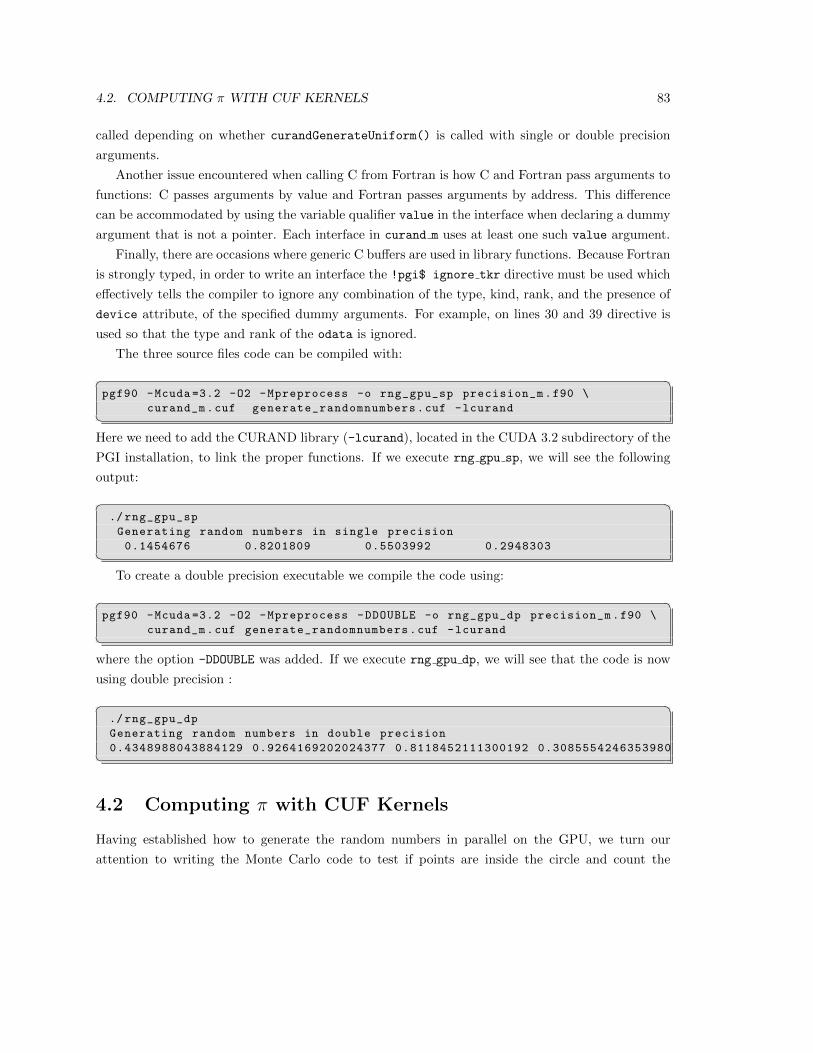
4.2. COMPUTING π WITH CUF KERNELS 83
called depending on whether curandGenerateUniform() is called with single or double precision
arguments.
Another issue encountered when calling C from Fortran is how C and Fortran pass arguments to
functions: C passes arguments by value and Fortran passes arguments by address. This difference
can be accommodated by using the variable qualifier value in the interface when declaring a dummy
argument that is not a pointer. Each interface in curand m uses at least one such value argument.
Finally, there are occasions where generic C buffers are used in library functions. Because Fortran
is strongly typed, in order to write an interface the !pgi$ ignore tkr directive must be used which
effectively tells the compiler to ignore any combination of the type, kind, rank, and the presence of
device attribute, of the specified dummy arguments. For example, on lines 30 and 39 directive is
used so that the type and rank of the odata is ignored.
The three source files code can be compiled with:� �pgf90 -Mcuda =3.2 -O2 -Mpreprocess -o rng_gpu_sp precision_m.f90 \
curand_m.cuf generate_randomnumbers.cuf -lcurand�Here we need to add the CURAND library (-lcurand), located in the CUDA 3.2 subdirectory of the
PGI installation, to link the proper functions. If we execute rng gpu sp, we will see the following
output:� �./ rng_gpu_sp
Generating random numbers in single precision
0.1454676 0.8201809 0.5503992 0.2948303�To create a double precision executable we compile the code using:� �
pgf90 -Mcuda =3.2 -O2 -Mpreprocess -DDOUBLE -o rng_gpu_dp precision_m.f90 \
curand_m.cuf generate_randomnumbers.cuf -lcurand�where the option -DDOUBLE was added. If we execute rng gpu dp, we will see that the code is now
using double precision :� �./ rng_gpu_dp
Generating random numbers in double precision
0.4348988043884129 0.9264169202024377 0.8118452111300192 0.3085554246353980�4.2 Computing π with CUF Kernels
Having established how to generate the random numbers in parallel on the GPU, we turn our
attention to writing the Monte Carlo code to test if points are inside the circle and count the
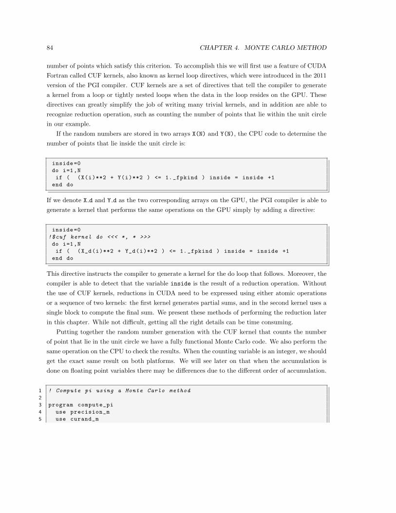
84 CHAPTER 4. MONTE CARLO METHOD
number of points which satisfy this criterion. To accomplish this we will first use a feature of CUDA
Fortran called CUF kernels, also known as kernel loop directives, which were introduced in the 2011
version of the PGI compiler. CUF kernels are a set of directives that tell the compiler to generate
a kernel from a loop or tightly nested loops when the data in the loop resides on the GPU. These
directives can greatly simplify the job of writing many trivial kernels, and in addition are able to
recognize reduction operation, such as counting the number of points that lie within the unit circle
in our example.
If the random numbers are stored in two arrays X(N) and Y(N), the CPU code to determine the
number of points that lie inside the unit circle is:
inside =0
do i=1,N
if ( (X(i)**2 + Y(i)**2 ) <= 1. _fpkind ) inside = inside +1
end do
If we denote X d and Y d as the two corresponding arrays on the GPU, the PGI compiler is able to
generate a kernel that performs the same operations on the GPU simply by adding a directive:
inside =0
!$cuf kernel do <<< *, * >>>
do i=1,N
if ( (X_d(i)**2 + Y_d(i)**2 ) <= 1. _fpkind ) inside = inside +1
end do
This directive instructs the compiler to generate a kernel for the do loop that follows. Moreover, the
compiler is able to detect that the variable inside is the result of a reduction operation. Without
the use of CUF kernels, reductions in CUDA need to be expressed using either atomic operations
or a sequence of two kernels: the first kernel generates partial sums, and in the second kernel uses a
single block to compute the final sum. We present these methods of performing the reduction later
in this chapter. While not difficult, getting all the right details can be time consuming.
Putting together the random number generation with the CUF kernel that counts the number
of point that lie in the unit circle we have a fully functional Monte Carlo code. We also perform the
same operation on the CPU to check the results. When the counting variable is an integer, we should
get the exact same result on both platforms. We will see later on that when the accumulation is
done on floating point variables there may be differences due to the different order of accumulation.
1 ! Compute pi using a Monte Carlo method
2
3 program compute_pi
4 use precision_m
5 use curand_m
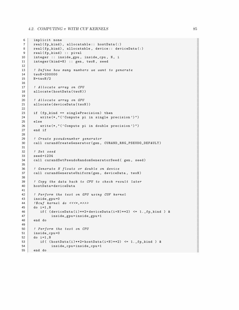
4.2. COMPUTING π WITH CUF KERNELS 85
6 implicit none
7 real(fp_kind), allocatable :: hostData (:)
8 real(fp_kind), allocatable , device :: deviceData (:)
9 real(fp_kind) :: pival
10 integer :: inside_gpu , inside_cpu , N, i
11 integer(kind =8) :: gen , twoN , seed
12
13 ! Define how many numbers we want to generate
14 twoN =200000
15 N=twoN/2
16
17 ! Allocate array on CPU
18 allocate(hostData(twoN))
19
20 ! Allocate array on GPU
21 allocate(deviceData(twoN))
22
23 if (fp_kind == singlePrecision) then
24 write(*,"(’Compute pi in single precision ’)")
25 else
26 write(*,"(’Compute pi in double precision ’)")
27 end if
28
29 ! Create pseudonumber generator
30 call curandCreateGenerator(gen , CURAND_RNG_PSEUDO_DEFAULT)
31
32 ! Set seed
33 seed =1234
34 call curandSetPseudoRandomGeneratorSeed( gen , seed)
35
36 ! Generate N floats or double on device
37 call curandGenerateUniform(gen , deviceData , twoN)
38
39 ! Copy the data back to CPU to check result later
40 hostData=deviceData
41
42 ! Perform the test on GPU using CUF kernel
43 inside_gpu =0
44 !$cuf kernel do <<<*,*>>>
45 do i=1,N
46 if( (deviceData(i)**2+ deviceData(i+N)**2) <= 1. _fp_kind ) &
47 inside_gpu=inside_gpu +1
48 end do
49
50 ! Perform the test on CPU
51 inside_cpu =0
52 do i=1,N
53 if( (hostData(i)**2+ hostData(i+N)**2) <= 1. _fp_kind ) &
54 inside_cpu=inside_cpu +1
55 end do
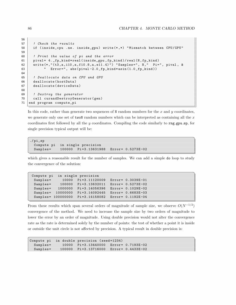
86 CHAPTER 4. MONTE CARLO METHOD
56
57 ! Check the results
58 if (inside_cpu .ne. inside_gpu) write (*,*) "Mismatch between CPU/GPU"
59
60 ! Print the value of pi and the error
61 pival= 4. _fp_kind*real(inside_gpu ,fp_kind )/real(N,fp_kind)
62 write(*,"(t3 ,a,i10 ,a,f10.8,a,e11.4)") "Samples=", N," Pi=", pival , &
63 " Error=", abs(pival -2.0 _fp_kind*asin (1.0 _fp_kind ))
64
65 ! Deallocate data on CPU and GPU
66 deallocate(hostData)
67 deallocate(deviceData)
68
69 ! Destroy the generator
70 call curandDestroyGenerator(gen)
71 end program compute_pi
In this code, rather than generate two sequences of N random numbers for the x and y coordinates,
we generate only one set of twoN random numbers which can be interpreted as containing all the x
coordinates first followed by all the y coordinates. Compiling the code similarly to rng gpu sp, for
single precision typical output will be:� �./pi_sp
Compute pi in single precision
Samples= 100000 Pi =3.13631988 Error= 0.5273E-02�which gives a reasonable result for the number of samples. We can add a simple do loop to study
the convergence of the solution:� �Compute pi in single precision
Samples= 10000 Pi =3.11120009 Error= 0.3039E-01
Samples= 100000 Pi =3.13632011 Error= 0.5273E-02
Samples= 1000000 Pi =3.14056396 Error= 0.1029E-02
Samples= 10000000 Pi =3.14092445 Error= 0.6683E-03
Samples= 100000000 Pi =3.14158082 Error= 0.1192E-04�From these results which span several orders of magnitude of sample size, we observe O(N−1/2)
convergence of the method. We need to increase the sample size by two orders of magnitude to
lower the error by an order of magnitude. Using double precision would not alter the convergence
rate as the rate is determined solely by the number of points: the test of whether a point it is inside
or outside the unit circle is not affected by precision. A typical result in double precision is:� �Compute pi in double precision (seed =1234)
Samples= 10000 Pi =3.13440000 Error= 0.7193E-02
Samples= 100000 Pi =3.13716000 Error= 0.4433E-02
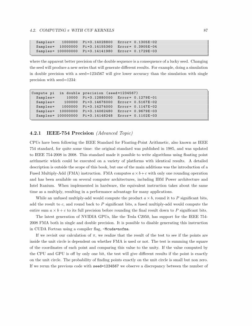
4.2. COMPUTING π WITH CUF KERNELS 87
Samples= 1000000 Pi =3.14028800 Error= 0.1305E-02
Samples= 10000000 Pi =3.14155360 Error= 0.3905E-04
Samples= 100000000 Pi =3.14141980 Error= 0.1729E-03�where the apparent better precision of the double sequence is a consequence of a lucky seed. Changing
the seed will produce a new series that will generate different results. For example, doing a simulation
in double precision with a seed=1234567 will give lower accuracy than the simulation with single
precision with seed=1234:
� �Compute pi in double precision (seed =1234567)
Samples= 10000 Pi =3.12880000 Error= 0.1279E-01
Samples= 100000 Pi =3.14676000 Error= 0.5167E-02
Samples= 1000000 Pi =3.14274000 Error= 0.1147E-02
Samples= 10000000 Pi =3.14062480 Error= 0.9679E-03
Samples= 100000000 Pi =3.14148248 Error= 0.1102E-03�4.2.1 IEEE-754 Precision (Advanced Topic)
CPUs have been following the IEEE Standard for Floating-Point Arithmetic, also known as IEEE
754 standard, for quite some time: the original standard was published in 1985, and was updated
to IEEE 754-2008 in 2008. This standard made it possible to write algorithms using floating point
arithmetic which could be executed on a variety of platforms with identical results. A detailed
description is outside the scope of this book, but one of the main additions was the introduction of a
Fused Multiply-Add (FMA) instruction. FMA computes a× b+ c with only one rounding operation
and has been available on several computer architectures, including IBM Power architecture and
Intel Itanium. When implemented in hardware, the equivalent instruction takes about the same
time as a multiply, resulting in a performance advantage for many applications.
While an unfused multiply-add would compute the product a× b, round it to P significant bits,
add the result to c, and round back to P significant bits, a fused multiply-add would compute the
entire sum a× b+ c to its full precision before rounding the final result down to P significant bits.
The latest generation of NVIDIA GPUs, like the Tesla C2050, has support for the IEEE 754-
2008 FMA both in single and double precision. It is possible to disable generating this instruction
in CUDA Fortran using a compiler flag, -Mcuda=nofma.
If we revisit our calculation of π, we realize that the result of the test to see if the points are
inside the unit circle is dependent on whether FMA is used or not. The test is summing the square
of the coordinates of each point and comparing this value to the unity. If the value computed by
the CPU and GPU is off by only one bit, the test will give different results if the point is exactly
on the unit circle. The probability of finding points exactly on the unit circle is small but non zero.
If we rerun the previous code with seed=1234567 we observe a discrepancy between the number of

88 CHAPTER 4. MONTE CARLO METHOD
interior points detected by the CPU and the one detected by the GPU when the number of samples
is equal to 100 million.� �Compute pi in single precision (seed =1234567 FMA enabled)
Samples= 10000 Pi =3.16720009 Error= 0.2561E-01
Samples= 100000 Pi =3.13919997 Error= 0.2393E-02
Samples= 1000000 Pi =3.14109206 Error= 0.5007E-03
Samples= 10000000 Pi =3.14106607 Error= 0.5267E-03
Mismatch between CPU/GPU 78534862 78534859
Samples= 100000000 Pi =3.14139414 Error= 0.1986E-03�There are 3 out of 100 million points for which the test is giving different results.
N x y x2 + y2 x2 + y2
CPU GPU with FMA2377069 6.162945032e-01 7.875158191e-01 1.000000000 1.000000119
3F1DC57A 3F499AA3 3F800000 3F80000133027844 2.018149495e-01 9.794237018e-01 1.000000000 1.000000119
3E4EA894 3F7ABB83 3F800000 3F80000181541078 6.925099492e-01 7.214083672e-01 1.000000000 1.000000119
3F314855 3F38AE38 3F800000 3F800001
Table 4.1: Coordinates of the points and distance from the origin with results different betweenCPU and GPU. Values are in floating point (top) and hexadecimal (bottom) representations.
We will analyze the error in detail for the first point, however the same analysis applies to the
other points. To analyze the error we look at results obtained by rearranging the order of the
multiplications and adds. Using the notation fma(a, b, c) = a× b+ c, we could compute x2 + y2 in
one of three ways:
1. Compute x ∗ x, compute y ∗ y and then add the two squares:
(x*x + y*y) = 1.000000000e+00 3f800000
2. Compute y ∗ y , use FMA(x,x,y*y)
fmaf(x,x,y*y)= 1.000000000e+00 3f800000
3. Compute x ∗ x , use FMA(y,y,x*x)
fmaf(y,y,x*x)= 1.000000119e+00 3f800001
In theory, the last way should be the most accurate as in this case y > x and therefore we are
using the full precision for the bigger term. To confirm this, we could try the following experiment:
What would it happen if we recompute the distance on the CPU in double precision?
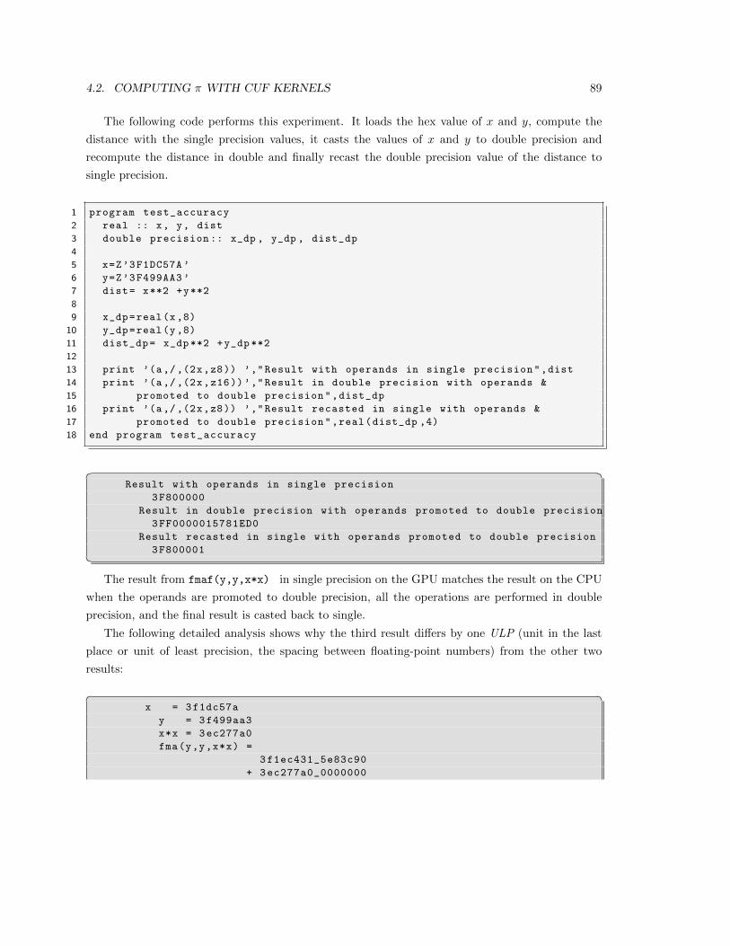
4.2. COMPUTING π WITH CUF KERNELS 89
The following code performs this experiment. It loads the hex value of x and y, compute the
distance with the single precision values, it casts the values of x and y to double precision and
recompute the distance in double and finally recast the double precision value of the distance to
single precision.
1 program test_accuracy
2 real :: x, y, dist
3 double precision :: x_dp , y_dp , dist_dp
4
5 x=Z’3F1DC57A ’
6 y=Z’3F499AA3 ’
7 dist= x**2 +y**2
8
9 x_dp=real(x,8)
10 y_dp=real(y,8)
11 dist_dp= x_dp **2 +y_dp **2
12
13 print ’(a,/,(2x,z8)) ’,"Result with operands in single precision",dist
14 print ’(a,/,(2x,z16))’,"Result in double precision with operands &
15 promoted to double precision",dist_dp
16 print ’(a,/,(2x,z8)) ’,"Result recasted in single with operands &
17 promoted to double precision",real(dist_dp ,4)
18 end program test_accuracy
� �Result with operands in single precision
3F800000
Result in double precision with operands promoted to double precision
3FF0000015781ED0
Result recasted in single with operands promoted to double precision
3F800001�The result from fmaf(y,y,x*x) in single precision on the GPU matches the result on the CPU
when the operands are promoted to double precision, all the operations are performed in double
precision, and the final result is casted back to single.
The following detailed analysis shows why the third result differs by one ULP (unit in the last
place or unit of least precision, the spacing between floating-point numbers) from the other two
results:� �x = 3f1dc57a
y = 3f499aa3
x*x = 3ec277a0
fma(y,y,x*x) =
3f1ec431_5e83c90
+ 3ec277a0_0000000
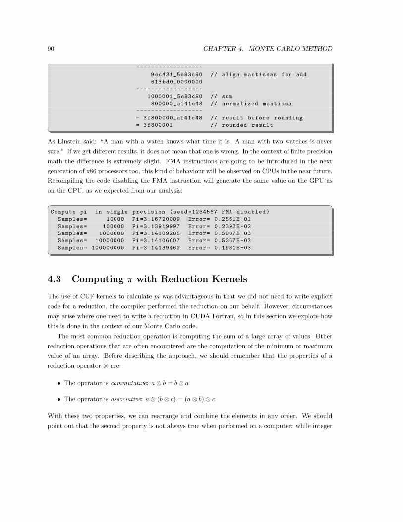
90 CHAPTER 4. MONTE CARLO METHOD
------------------
9ec431_5e83c90 // align mantissas for add
613 bd0_0000000
------------------
1000001 _5e83c90 // sum
800000 _af41e48 // normalized mantissa
------------------
= 3f800000_af41e48 // result before rounding
= 3f800001 // rounded result�As Einstein said: “A man with a watch knows what time it is. A man with two watches is never
sure.” If we get different results, it does not mean that one is wrong. In the context of finite precision
math the difference is extremely slight. FMA instructions are going to be introduced in the next
generation of x86 processors too, this kind of behaviour will be observed on CPUs in the near future.
Recompiling the code disabling the FMA instruction will generate the same value on the GPU as
on the CPU, as we expected from our analysis:� �Compute pi in single precision (seed =1234567 FMA disabled)
Samples= 10000 Pi =3.16720009 Error= 0.2561E-01
Samples= 100000 Pi =3.13919997 Error= 0.2393E-02
Samples= 1000000 Pi =3.14109206 Error= 0.5007E-03
Samples= 10000000 Pi =3.14106607 Error= 0.5267E-03
Samples= 100000000 Pi =3.14139462 Error= 0.1981E-03�4.3 Computing π with Reduction Kernels
The use of CUF kernels to calculate pi was advantageous in that we did not need to write explicit
code for a reduction, the compiler performed the reduction on our behalf. However, circumstances
may arise where one need to write a reduction in CUDA Fortran, so in this section we explore how
this is done in the context of our Monte Carlo code.
The most common reduction operation is computing the sum of a large array of values. Other
reduction operations that are often encountered are the computation of the minimum or maximum
value of an array. Before describing the approach, we should remember that the properties of a
reduction operator ⊗ are:
• The operator is commutative: a⊗ b = b⊗ a
• The operator is associative: a⊗ (b⊗ c) = (a⊗ b)⊗ c
With these two properties, we can rearrange and combine the elements in any order. We should
point out that the second property is not always true when performed on a computer: while integer
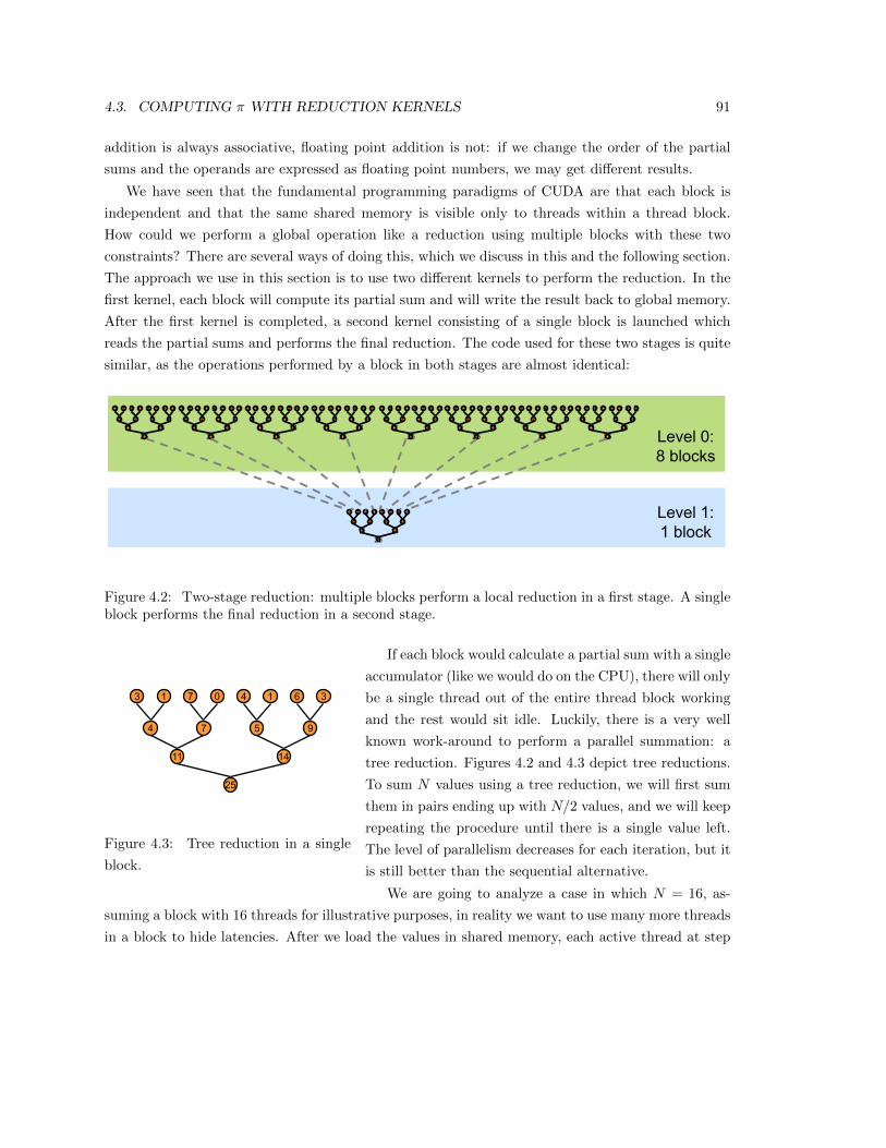
4.3. COMPUTING π WITH REDUCTION KERNELS 91
addition is always associative, floating point addition is not: if we change the order of the partial
sums and the operands are expressed as floating point numbers, we may get different results.
We have seen that the fundamental programming paradigms of CUDA are that each block is
independent and that the same shared memory is visible only to threads within a thread block.
How could we perform a global operation like a reduction using multiple blocks with these two
constraints? There are several ways of doing this, which we discuss in this and the following section.
The approach we use in this section is to use two different kernels to perform the reduction. In the
first kernel, each block will compute its partial sum and will write the result back to global memory.
After the first kernel is completed, a second kernel consisting of a single block is launched which
reads the partial sums and performs the final reduction. The code used for these two stages is quite
similar, as the operations performed by a block in both stages are almost identical:
5
Solution: Kernel Decomposition
Avoid global sync by decomposing computation into multiple kernel invocations
In the case of reductions, code for all levels is the same
Recursive kernel invocation
4 7 5 911 14
25
3 1 7 0 4 1 6 34 7 5 9
11 1425
3 1 7 0 4 1 6 34 7 5 9
11 1425
3 1 7 0 4 1 6 34 7 5 9
11 1425
3 1 7 0 4 1 6 34 7 5 9
11 1425
3 1 7 0 4 1 6 34 7 5 9
11 1425
3 1 7 0 4 1 6 34 7 5 9
11 1425
3 1 7 0 4 1 6 34 7 5 9
11 1425
3 1 7 0 4 1 6 3
4 7 5 911 14
25
3 1 7 0 4 1 6 3
Level 0:8 blocks
Level 1:1 block
Figure 4.2: Two-stage reduction: multiple blocks perform a local reduction in a first stage. A singleblock performs the final reduction in a second stage.
3
Parallel Reduction
Tree-based approach used within each thread block
Need to be able to use multiple thread blocksTo process very large arraysTo keep all multiprocessors on the GPU busyEach thread block reduces a portion of the array
But how do we communicate partial results between thread blocks?
4 7 5 9
11 14
25
3 1 7 0 4 1 6 3
Figure 4.3: Tree reduction in a single
block.
If each block would calculate a partial sum with a single
accumulator (like we would do on the CPU), there will only
be a single thread out of the entire thread block working
and the rest would sit idle. Luckily, there is a very well
known work-around to perform a parallel summation: a
tree reduction. Figures 4.2 and 4.3 depict tree reductions.
To sum N values using a tree reduction, we will first sum
them in pairs ending up with N/2 values, and we will keep
repeating the procedure until there is a single value left.
The level of parallelism decreases for each iteration, but it
is still better than the sequential alternative.
We are going to analyze a case in which N = 16, as-
suming a block with 16 threads for illustrative purposes, in reality we want to use many more threads
in a block to hide latencies. After we load the values in shared memory, each active thread at step
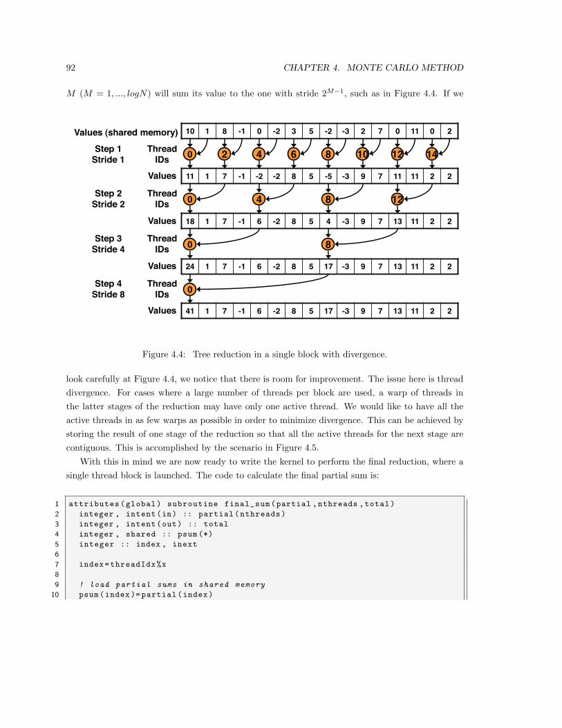
92 CHAPTER 4. MONTE CARLO METHOD
M (M = 1, ..., logN) will sum its value to the one with stride 2M−1, such as in Figure 4.4. If we
8
Parallel Reduction: Interleaved Addressing
10 1 8 -1 0 -2 3 5 -2 -3 2 7 0 11 0 2Values (shared memory)
0 2 4 6 8 10 12 14
11 1 7 -1 -2 -2 8 5 -5 -3 9 7 11 11 2 2Values
0 4 8 12
18 1 7 -1 6 -2 8 5 4 -3 9 7 13 11 2 2Values
0 8
24 1 7 -1 6 -2 8 5 17 -3 9 7 13 11 2 2Values
0
41 1 7 -1 6 -2 8 5 17 -3 9 7 13 11 2 2Values
Thread IDs
Step 1 Stride 1
Step 2 Stride 2
Step 3 Stride 4
Step 4 Stride 8
Thread IDs
Thread IDs
Thread IDs
Figure 4.4: Tree reduction in a single block with divergence.
look carefully at Figure 4.4, we notice that there is room for improvement. The issue here is thread
divergence. For cases where a large number of threads per block are used, a warp of threads in
the latter stages of the reduction may have only one active thread. We would like to have all the
active threads in as few warps as possible in order to minimize divergence. This can be achieved by
storing the result of one stage of the reduction so that all the active threads for the next stage are
contiguous. This is accomplished by the scenario in Figure 4.5.
With this in mind we are now ready to write the kernel to perform the final reduction, where a
single thread block is launched. The code to calculate the final partial sum is:
1 attributes(global) subroutine final_sum(partial ,nthreads ,total)
2 integer , intent(in) :: partial(nthreads)
3 integer , intent(out) :: total
4 integer , shared :: psum (*)
5 integer :: index , inext
6
7 index=threadIdx%x
8
9 ! load partial sums in shared memory
10 psum(index)= partial(index)
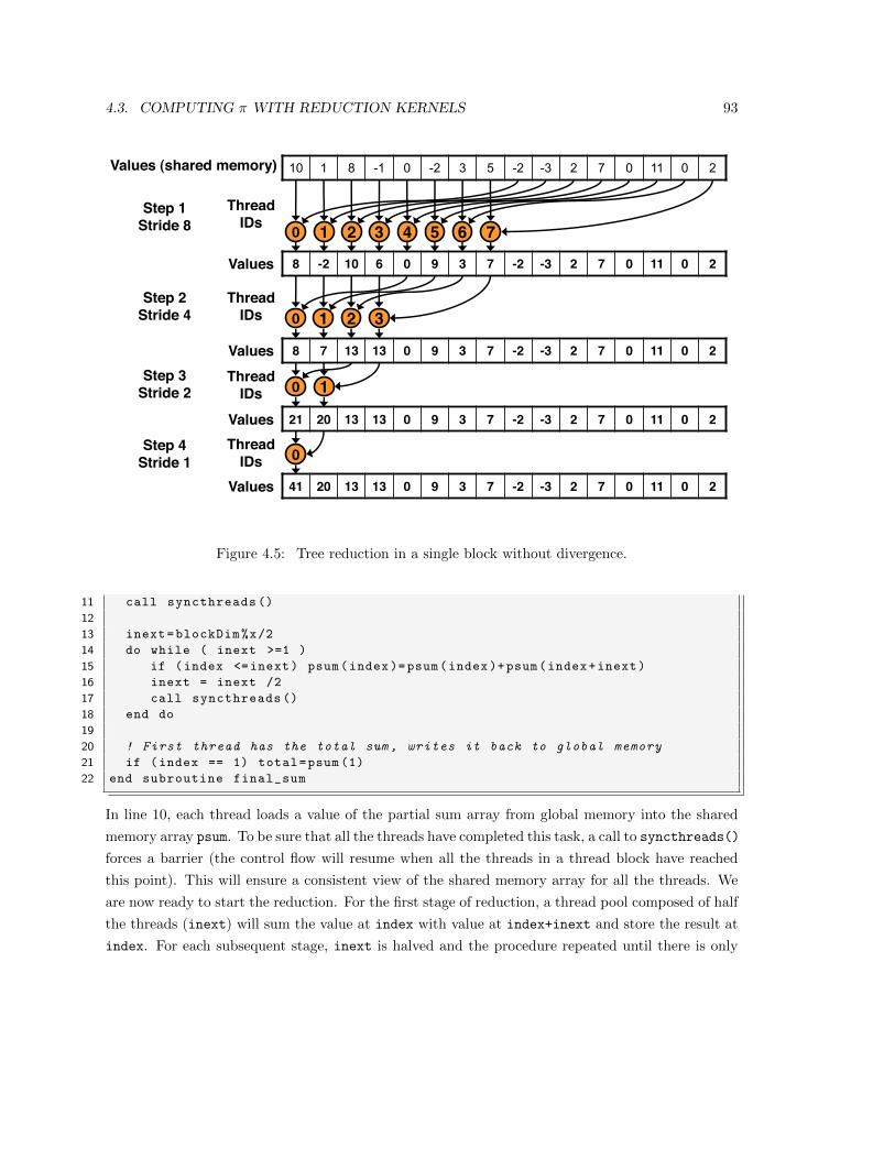
4.3. COMPUTING π WITH REDUCTION KERNELS 93
14
Parallel Reduction: Sequential Addressing
10 1 8 -1 0 -2 3 5 -2 -3 2 7 0 11 0 2Values (shared memory)
0 1 2 3 4 5 6 7
8 -2 10 6 0 9 3 7 -2 -3 2 7 0 11 0 2Values
0 1 2 3
8 7 13 13 0 9 3 7 -2 -3 2 7 0 11 0 2Values
0 1
21 20 13 13 0 9 3 7 -2 -3 2 7 0 11 0 2Values
0
41 20 13 13 0 9 3 7 -2 -3 2 7 0 11 0 2Values
Thread IDs
Step 1 Stride 8
Step 2 Stride 4
Step 3 Stride 2
Step 4 Stride 1
Thread IDs
Thread IDs
Thread IDs
Sequential addressing is conflict freeFigure 4.5: Tree reduction in a single block without divergence.
11 call syncthreads ()
12
13 inext=blockDim%x/2
14 do while ( inext >=1 )
15 if (index <=inext) psum(index )=psum(index )+psum(index+inext)
16 inext = inext /2
17 call syncthreads ()
18 end do
19
20 ! First thread has the total sum , writes it back to global memory
21 if (index == 1) total=psum (1)
22 end subroutine final_sum
In line 10, each thread loads a value of the partial sum array from global memory into the shared
memory array psum. To be sure that all the threads have completed this task, a call to syncthreads()
forces a barrier (the control flow will resume when all the threads in a thread block have reached
this point). This will ensure a consistent view of the shared memory array for all the threads. We
are now ready to start the reduction. For the first stage of reduction, a thread pool composed of half
the threads (inext) will sum the value at index with value at index+inext and store the result at
index. For each subsequent stage, inext is halved and the procedure repeated until there is only
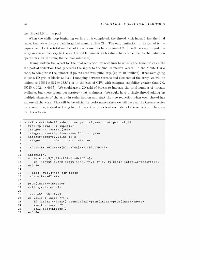
94 CHAPTER 4. MONTE CARLO METHOD
one thread left in the pool.
When the while loop beginning on line 14 is completed, the thread with index 1 has the final
value, that we will store back in global memory (line 21). The only limitation in the kernel is the
requirement for the total number of threads used to be a power of 2. It will be easy to pad the
array in shared memory to the next suitable number with values that are neutral to the reduction
operation ( for the sum, the neutral value is 0).
Having written the kernel for the final reduction, we now turn to writing the kernel to calculate
the partial reduction that generates the input to the final reduction kernel. In the Monte Carlo
code, to compute π the number of points used was quite large (up to 100 million). If we were going
to use a 1D grid of blocks and a 1:1 mapping between threads and elements of the array, we will be
limited to 65535 × 512 ≈ 33M ( or in the case of GPU with compute capability greater than 2.0,
65535 × 1024 ≈ 66M). We could use a 2D grid of blocks to increase the total number of threads
available, but there is another strategy that is simpler. We could have a single thread adding up
multiple elements of the array in serial fashion and start the tree reduction when each thread has
exhausted the work. This will be beneficial for performance since we will have all the threads active
for a long time, instead of losing half of the active threads at each step of the reduction. The code
for this is below:
1 attributes(global) subroutine partial_sum(input ,partial ,N)
2 real(fp_kind) :: input(N)
3 integer :: partial (256)
4 integer , shared , dimension (256) :: psum
5 integer(kind=8), value :: N
6 integer :: i,index , inext ,interior
7
8 index=threadIdx%x+( BlockIdx%x-1)* BlockDim%x
9
10 interior =0
11 do i=index ,N/2,BlockDim%x*GridDim%x
12 if( (input(i)**2+ input(i+N/2)**2) <= 1. _fp_kind) interior=interior +1
13 end do
14
15 ! Local reduction per block
16 index=threadIdx%x
17
18 psum(index)= interior
19 call syncthreads ()
20
21 inext=blockDim%x/2
22 do while ( inext >=1 )
23 if (index <=inext) psum(index )=psum(index )+psum(index+inext)
24 inext = inext /2
25 call syncthreads ()
26 end do
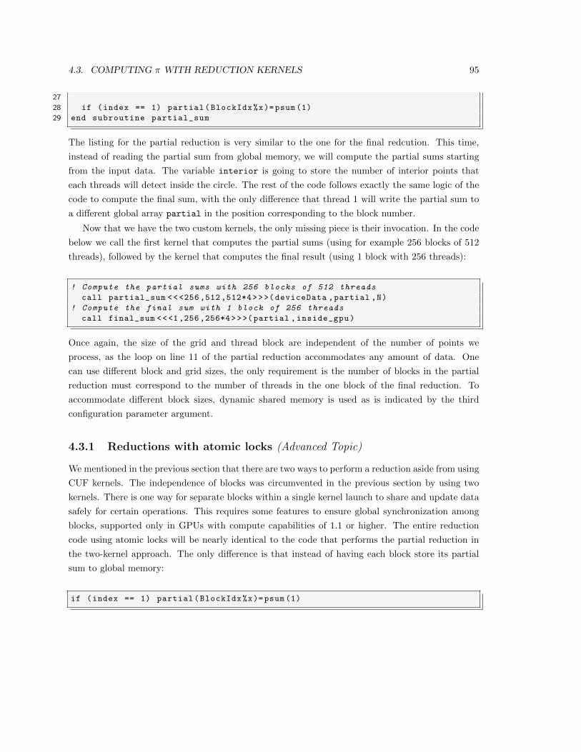
4.3. COMPUTING π WITH REDUCTION KERNELS 95
27
28 if (index == 1) partial(BlockIdx%x)=psum (1)
29 end subroutine partial_sum
The listing for the partial reduction is very similar to the one for the final redcution. This time,
instead of reading the partial sum from global memory, we will compute the partial sums starting
from the input data. The variable interior is going to store the number of interior points that
each threads will detect inside the circle. The rest of the code follows exactly the same logic of the
code to compute the final sum, with the only difference that thread 1 will write the partial sum to
a different global array partial in the position corresponding to the block number.
Now that we have the two custom kernels, the only missing piece is their invocation. In the code
below we call the first kernel that computes the partial sums (using for example 256 blocks of 512
threads), followed by the kernel that computes the final result (using 1 block with 256 threads):
! Compute the partial sums with 256 blocks of 512 threads
call partial_sum <<<256,512,512*4>>>( deviceData ,partial ,N)
! Compute the final sum with 1 block of 256 threads
call final_sum <<<1,256,256*4>>>(partial ,inside_gpu)
Once again, the size of the grid and thread block are independent of the number of points we
process, as the loop on line 11 of the partial reduction accommodates any amount of data. One
can use different block and grid sizes, the only requirement is the number of blocks in the partial
reduction must correspond to the number of threads in the one block of the final reduction. To
accommodate different block sizes, dynamic shared memory is used as is indicated by the third
configuration parameter argument.
4.3.1 Reductions with atomic locks (Advanced Topic)
We mentioned in the previous section that there are two ways to perform a reduction aside from using
CUF kernels. The independence of blocks was circumvented in the previous section by using two
kernels. There is one way for separate blocks within a single kernel launch to share and update data
safely for certain operations. This requires some features to ensure global synchronization among
blocks, supported only in GPUs with compute capabilities of 1.1 or higher. The entire reduction
code using atomic locks will be nearly identical to the code that performs the partial reduction in
the two-kernel approach. The only difference is that instead of having each block store its partial
sum to global memory:
if (index == 1) partial(BlockIdx%x)=psum (1)
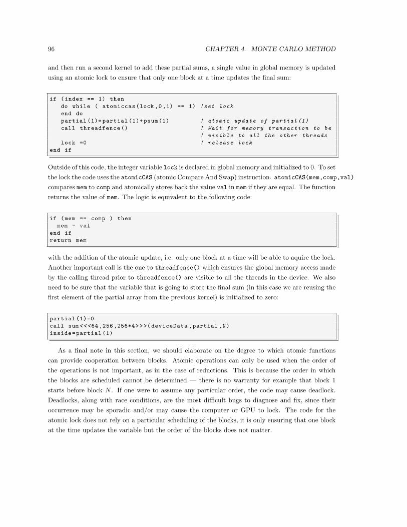
96 CHAPTER 4. MONTE CARLO METHOD
and then run a second kernel to add these partial sums, a single value in global memory is updated
using an atomic lock to ensure that only one block at a time updates the final sum:
if (index == 1) then
do while ( atomiccas(lock ,0,1) == 1) !set lock
end do
partial (1)= partial (1)+ psum (1) ! atomic update of partial (1)
call threadfence () ! Wait for memory transaction to be
! visible to all the other threads
lock =0 ! release lock
end if
Outside of this code, the integer variable lock is declared in global memory and initialized to 0. To set
the lock the code uses the atomicCAS (atomic Compare And Swap) instruction. atomicCAS(mem,comp,val)
compares mem to comp and atomically stores back the value val in mem if they are equal. The function
returns the value of mem. The logic is equivalent to the following code:
if (mem == comp ) then
mem = val
end if
return mem
with the addition of the atomic update, i.e. only one block at a time will be able to aquire the lock.
Another important call is the one to threadfence() which ensures the global memory access made
by the calling thread prior to threadfence() are visible to all the threads in the device. We also
need to be sure that the variable that is going to store the final sum (in this case we are reusing the
first element of the partial array from the previous kernel) is initialized to zero:
partial (1)=0
call sum <<<64,256,256*4>>>( deviceData ,partial ,N)
inside=partial (1)
As a final note in this section, we should elaborate on the degree to which atomic functions
can provide cooperation between blocks. Atomic operations can only be used when the order of
the operations is not important, as in the case of reductions. This is because the order in which
the blocks are scheduled cannot be determined — there is no warranty for example that block 1
starts before block N . If one were to assume any particular order, the code may cause deadlock.
Deadlocks, along with race conditions, are the most difficult bugs to diagnose and fix, since their
occurrence may be sporadic and/or may cause the computer or GPU to lock. The code for the
atomic lock does not rely on a particular scheduling of the blocks, it is only ensuring that one block
at the time updates the variable but the order of the blocks does not matter.

4.3. COMPUTING π WITH REDUCTION KERNELS 97
4.3.2 Accuracy of reduction (Advanced Topic)
4.3.3 Performance comparison

98 CHAPTER 4. MONTE CARLO METHOD
Chapter 5
Finite Difference Method
In many fields of science and engineering the governing system of equations take the form of either
ordinary or partial differential equations. One method of solving these equations is using finite
differences, where the continuous analytical derivatives are approximated at each point on a discrete
grid using values of neighboring points.
5.1 Problem Statement
Our example uses a three-dimensional grid of size 643. For simplicity we assume periodic boundary
conditions and only consider first-order derivatives, although extending the code to calculate higher-
order derivatives with other types of boundary conditions is straightforward.
The finite difference method essentially uses a weighted summation of function values at neigh-
boring points to approximate the derivative at a particular point. For a (2N + 1)-point stencil with
a uniform spacing ∆x in the x-direction, a central finite difference scheme for the derivative in x
can be written as:
∂f(x, y, z)
∂x≈ 1
∆x
N∑i=−N
Cif(x+ i∆x, y, z)
and similarly for other directions. The coefficients Ci are typically generated from Taylor series
expansions and can be chosen to obtain a scheme with desired characteristics such as accuracy,
and in the context of partial differential equations, dispersion and dissipation. For explicit finite
difference schemes such as the type above, larger stencils typically have a higher order of accuracy.
For this study we use a nine-point stencil which has an eighth-order accuracy. We also choose a
symmetric stencil, which can be written as:
∂fi,j,k∂x
≈ ax (fi+1,j,k − fi−1,j,k)+bx (fi+2,j,k − fi−2,j,k)+cx (fi+3,j,k − fi−3,j,k)+dx (fi+4,j,k − fi−4,j,k)
99
100 CHAPTER 5. FINITE DIFFERENCE METHOD
where we specify values of the function on the computational grid using the grid indices i, j, k rather
than the physical coordinates x, y, z. Here the coefficients are ax = 45
1∆x , bx = − 1
51
∆x , cx = 4105
1∆x ,
and dx = − 1280
1∆x , which is a typical eighth-order scheme. For derivative in the y- and z-directions
the index offsets in the above equation are simply applied to the j and k indices and the coefficients
are the same except ∆y and ∆z are used in place of ∆x.
Because we calculate an approximation to the derivative at each point on the 643 periodic grid,
the value of f at each point is used eight times, one time for each right-hand side term in the above
expression. In designing a derivative kernel, we want to exploit this data reuse by fetching the values
of f from global memory as few times as possible using shared memory.
5.2 Data Reuse and Shared Memory
Each block of threads can bring in a tile of data to shared memory, and then each thread in the
block can access all elements of the shared memory tile as needed. How does one choose the best tile
shape and size? Some experimentation is required, but characteristics of the finite difference-stencil
and grid size provide some direction.
When choosing a tile shape for stencil calculations, there typically is an overlap of the tiles
corresponding to half of the stencil size, as depicted on the right in Figure 5.1. Here, in order to
calculate the derivative in a 16× 16 tile (in yellow), the values of f not only from this tile but also
from two additional 4× 16 sections (in orange) must be loaded by each thread block. Overall, the f
values in the orange sections get loaded twice, once by the thread block that calculates the derivative
at that location, and once by the neighboring thread block. As a result, 8×16 values out of 16×16,
or half of the values, get loaded from global memory twice. In addition, coalescing on a device with
a compute capability of 2.x will be suboptimal for a 16 × 16 tile since perfect coalescing on such
devices requires access to data within 32 contiguous elements in global memory per load.
A better choice of tile (and thread block) which calculates the derivative at the same number
of points as above is depicted on the right of Figure 5.1. This tile avoids overlap altogether when
calculating the x-derivative for our one-dimensional stencil on a grid of 643 since the tile contains
all points in the direction of the derivative, as in the 64× 4 tile shown. A minimal tile would have
just one pencil, i.e. one-dimensional array of all points in a direction, however this would correspond
to a thread blocks of 64 threads, so from an occupancy standpoint it is beneficial to use multiple
pencils in a tile. In our finite difference code, which is listed in its entirety in Appendix B.3, we
parameterize the number of pencils to allow some experimentation. In addition to loading each value
of f only once, every warp of threads will load contiguous data from global memory using this tile
and therefore will result in perfectly coalesced accesses to global memory.
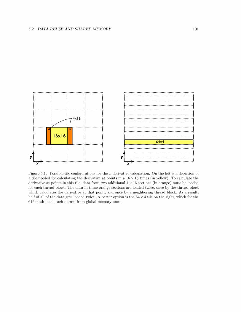
5.2. DATA REUSE AND SHARED MEMORY 101
16x16
4x16
64x4
x
y
x
y
Figure 5.1: Possible tile configurations for the x-derivative calculation. On the left is a depiction ofa tile needed for calculating the derivative at points in a 16× 16 times (in yellow). To calculate thederivative at points in this tile, data from two additional 4× 16 sections (in orange) must be loadedfor each thread block. The data in these orange sections are loaded twice, once by the thread blockwhich calculates the derivative at that point, and once by a neighboring thread block. As a result,half of all of the data gets loaded twice. A better option is the 64× 4 tile on the right, which for the643 mesh loads each datum from global memory once.
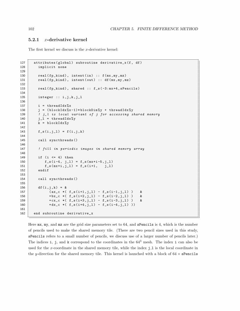
102 CHAPTER 5. FINITE DIFFERENCE METHOD
5.2.1 x-derivative kernel
The first kernel we discuss is the x-derivative kernel:
127 attributes(global) subroutine derivative_x(f, df)
128 implicit none
129
130 real(fp_kind), intent(in) :: f(mx,my,mz)
131 real(fp_kind), intent(out) :: df(mx,my,mz)
132
133 real(fp_kind), shared :: f_s(-3:mx+4,sPencils)
134
135 integer :: i,j,k,j_l
136
137 i = threadIdx%x
138 j = (blockIdx%x-1)* blockDim%y + threadIdx%y
139 ! j_l is local variant of j for accessing shared memory
140 j_l = threadIdx%y
141 k = blockIdx%y
142
143 f_s(i,j_l) = f(i,j,k)
144
145 call syncthreads ()
146
147 ! fill in periodic images in shared memory array
148
149 if (i <= 4) then
150 f_s(i-4, j_l) = f_s(mx+i-5,j_l)
151 f_s(mx+i,j_l) = f_s(i+1, j_l)
152 endif
153
154 call syncthreads ()
155
156 df(i,j,k) = &
157 (ax_c *( f_s(i+1,j_l) - f_s(i-1,j_l) ) &
158 +bx_c *( f_s(i+2,j_l) - f_s(i-2,j_l) ) &
159 +cx_c *( f_s(i+3,j_l) - f_s(i-3,j_l) ) &
160 +dx_c *( f_s(i+4,j_l) - f_s(i-4,j_l) ))
161
162 end subroutine derivative_x
Here mx, my, and mz are the grid size parameters set to 64, and sPencils is 4, which is the number
of pencils used to make the shared memory tile. (There are two pencil sizes used in this study,
sPencils refers to a small number of pencils, we discuss use of a larger number of pencils later.)
The indices i, j, and k correspond to the coordinates in the 643 mesh. The index i can also be
used for the x-coordinate in the shared memory tile, while the index j l is the local coordinate in
the y-direction for the shared memory tile. This kernel is launched with a block of 64 × sPencils
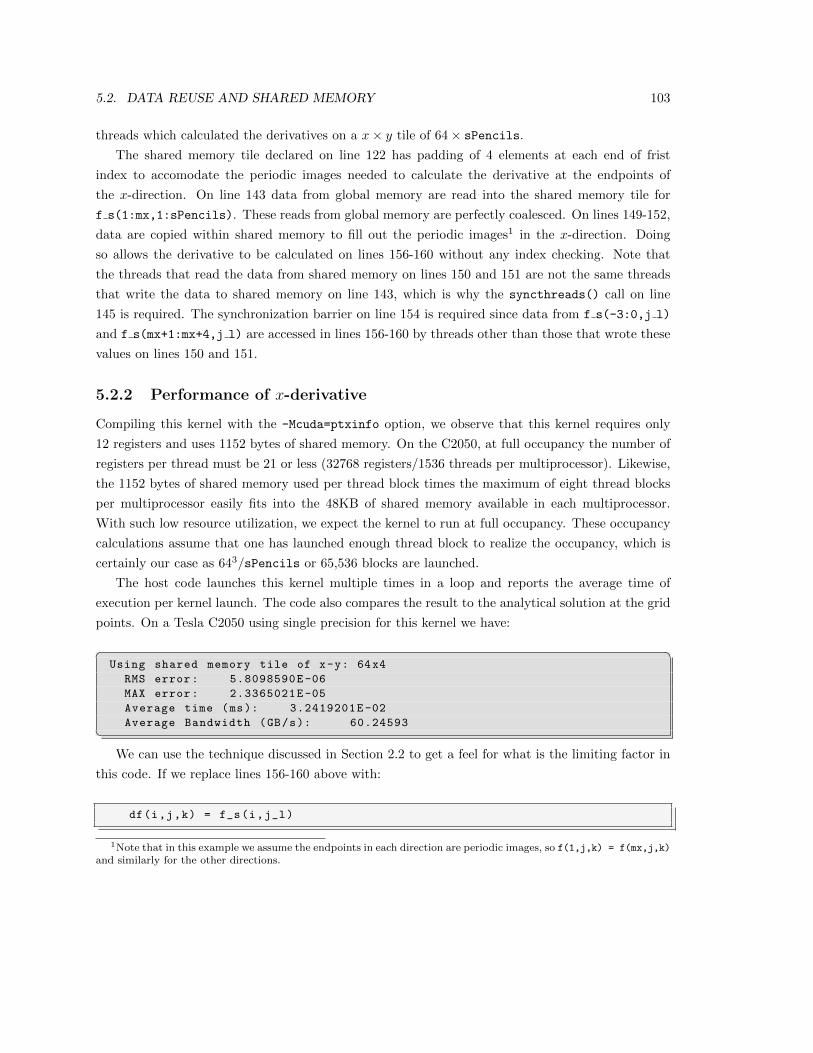
5.2. DATA REUSE AND SHARED MEMORY 103
threads which calculated the derivatives on a x× y tile of 64× sPencils.
The shared memory tile declared on line 122 has padding of 4 elements at each end of frist
index to accomodate the periodic images needed to calculate the derivative at the endpoints of
the x-direction. On line 143 data from global memory are read into the shared memory tile for
f s(1:mx,1:sPencils). These reads from global memory are perfectly coalesced. On lines 149-152,
data are copied within shared memory to fill out the periodic images1 in the x-direction. Doing
so allows the derivative to be calculated on lines 156-160 without any index checking. Note that
the threads that read the data from shared memory on lines 150 and 151 are not the same threads
that write the data to shared memory on line 143, which is why the syncthreads() call on line
145 is required. The synchronization barrier on line 154 is required since data from f s(-3:0,j l)
and f s(mx+1:mx+4,j l) are accessed in lines 156-160 by threads other than those that wrote these
values on lines 150 and 151.
5.2.2 Performance of x-derivative
Compiling this kernel with the -Mcuda=ptxinfo option, we observe that this kernel requires only
12 registers and uses 1152 bytes of shared memory. On the C2050, at full occupancy the number of
registers per thread must be 21 or less (32768 registers/1536 threads per multiprocessor). Likewise,
the 1152 bytes of shared memory used per thread block times the maximum of eight thread blocks
per multiprocessor easily fits into the 48KB of shared memory available in each multiprocessor.
With such low resource utilization, we expect the kernel to run at full occupancy. These occupancy
calculations assume that one has launched enough thread block to realize the occupancy, which is
certainly our case as 643/sPencils or 65,536 blocks are launched.
The host code launches this kernel multiple times in a loop and reports the average time of
execution per kernel launch. The code also compares the result to the analytical solution at the grid
points. On a Tesla C2050 using single precision for this kernel we have:� �Using shared memory tile of x-y: 64x4
RMS error: 5.8098590E-06
MAX error: 2.3365021E-05
Average time (ms): 3.2419201E-02
Average Bandwidth (GB/s): 60.24593�We can use the technique discussed in Section 2.2 to get a feel for what is the limiting factor in
this code. If we replace lines 156-160 above with:
df(i,j,k) = f_s(i,j_l)
1Note that in this example we assume the endpoints in each direction are periodic images, so f(1,j,k) = f(mx,j,k)
and similarly for the other directions.
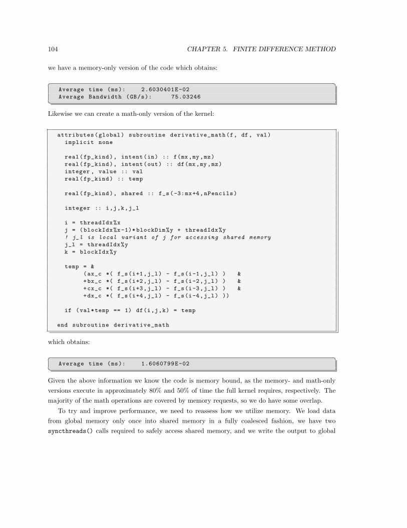
104 CHAPTER 5. FINITE DIFFERENCE METHOD
we have a memory-only version of the code which obtains:
� �Average time (ms): 2.6030401E-02
Average Bandwidth (GB/s): 75.03246�Likewise we can create a math-only version of the kernel:
attributes(global) subroutine derivative_math(f, df , val)
implicit none
real(fp_kind), intent(in) :: f(mx,my,mz)
real(fp_kind), intent(out) :: df(mx,my,mz)
integer , value :: val
real(fp_kind) :: temp
real(fp_kind), shared :: f_s(-3:mx+4,nPencils)
integer :: i,j,k,j_l
i = threadIdx%x
j = (blockIdx%x-1)* blockDim%y + threadIdx%y
! j_l is local variant of j for accessing shared memory
j_l = threadIdx%y
k = blockIdx%y
temp = &
(ax_c *( f_s(i+1,j_l) - f_s(i-1,j_l) ) &
+bx_c *( f_s(i+2,j_l) - f_s(i-2,j_l) ) &
+cx_c *( f_s(i+3,j_l) - f_s(i-3,j_l) ) &
+dx_c *( f_s(i+4,j_l) - f_s(i-4,j_l) ))
if (val*temp == 1) df(i,j,k) = temp
end subroutine derivative_math
which obtains:
� �Average time (ms): 1.6060799E-02�
Given the above information we know the code is memory bound, as the memory- and math-only
versions execute in approximately 80% and 50% of time the full kernel requires, respectively. The
majority of the math operations are covered by memory requests, so we do have some overlap.
To try and improve performance, we need to reassess how we utilize memory. We load data
from global memory only once into shared memory in a fully coalesced fashion, we have two
syncthreads() calls required to safely access shared memory, and we write the output to global
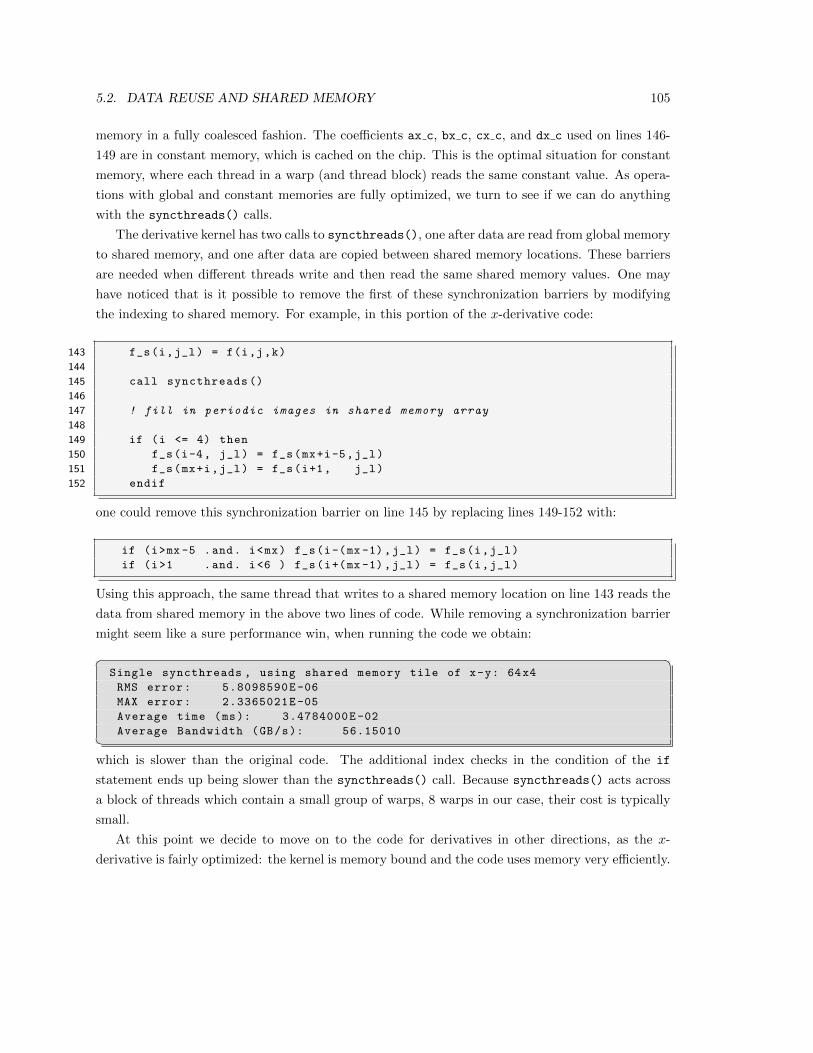
5.2. DATA REUSE AND SHARED MEMORY 105
memory in a fully coalesced fashion. The coefficients ax c, bx c, cx c, and dx c used on lines 146-
149 are in constant memory, which is cached on the chip. This is the optimal situation for constant
memory, where each thread in a warp (and thread block) reads the same constant value. As opera-
tions with global and constant memories are fully optimized, we turn to see if we can do anything
with the syncthreads() calls.
The derivative kernel has two calls to syncthreads(), one after data are read from global memory
to shared memory, and one after data are copied between shared memory locations. These barriers
are needed when different threads write and then read the same shared memory values. One may
have noticed that is it possible to remove the first of these synchronization barriers by modifying
the indexing to shared memory. For example, in this portion of the x-derivative code:
143 f_s(i,j_l) = f(i,j,k)
144
145 call syncthreads ()
146
147 ! fill in periodic images in shared memory array
148
149 if (i <= 4) then
150 f_s(i-4, j_l) = f_s(mx+i-5,j_l)
151 f_s(mx+i,j_l) = f_s(i+1, j_l)
152 endif
one could remove this synchronization barrier on line 145 by replacing lines 149-152 with:
if (i>mx -5 .and. i<mx) f_s(i-(mx -1),j_l) = f_s(i,j_l)
if (i>1 .and. i<6 ) f_s(i+(mx -1),j_l) = f_s(i,j_l)
Using this approach, the same thread that writes to a shared memory location on line 143 reads the
data from shared memory in the above two lines of code. While removing a synchronization barrier
might seem like a sure performance win, when running the code we obtain:� �Single syncthreads , using shared memory tile of x-y: 64x4
RMS error: 5.8098590E-06
MAX error: 2.3365021E-05
Average time (ms): 3.4784000E-02
Average Bandwidth (GB/s): 56.15010�which is slower than the original code. The additional index checks in the condition of the if
statement ends up being slower than the syncthreads() call. Because syncthreads() acts across
a block of threads which contain a small group of warps, 8 warps in our case, their cost is typically
small.
At this point we decide to move on to the code for derivatives in other directions, as the x-
derivative is fairly optimized: the kernel is memory bound and the code uses memory very efficiently.
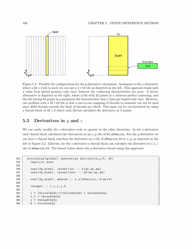
106 CHAPTER 5. FINITE DIFFERENCE METHOD
32x64
32x8
Thread Block
x
y
Tile
x
y
4x64
Figure 5.2: Possible tile configurations for the y-derivative calculation. Analogous to the x-derivativewhere a 64× 4 tile is used, we can use a 4× 64 tile as depicted on the left. This approach loads eachf value from global memory only once, however the coalescing characteristics are poor. A betteralternative is depicted on the right, where a tile with 32 points in x achieves perfect coalescing, andthe tile having 64 points in y maintains the characteristic that f data get loaded only once. However,one problem with a 32× 64 tile is that a one-to-one mapping of threads to elements can not be usedsince 2048 threads exceeds the limit of threads per block. This issue can be circumvented by usinga thread block of 32× 8 where each thread calculates the derivative at 8 points.
5.3 Derivatives in y and z
We can easily modify the x-derivative code to operate in the other directions. In the x-derivative
each thread block calculated the derivatives in an x, y tile of 64, sPencils. For the y-derivative we
can have a thread block calculate the derivative on a tile of sPencils, 64 in x, y, as depicted on the
left in Figure 5.2. Likewise, for the z-derivative a thread block can calculate the derivative in a x, z
tile of sPencils, 64. The kernel below shows the y-derivative kernel using this approach.
253 attributes(global) subroutine derivative_y(f, df)
254 implicit none
255
256 real(fp_kind), intent(in) :: f(mx,my,mz)
257 real(fp_kind), intent(out) :: df(mx,my,mz)
258
259 real(fp_kind), shared :: f_s(sPencils ,-3:my+4)
260
261 integer :: i,i_l ,j,k
262
263 i = (blockIdx%x-1)* blockDim%x + threadIdx%x
264 i_l = threadIdx%x
265 j = threadIdx%y
266 k = blockIdx%y
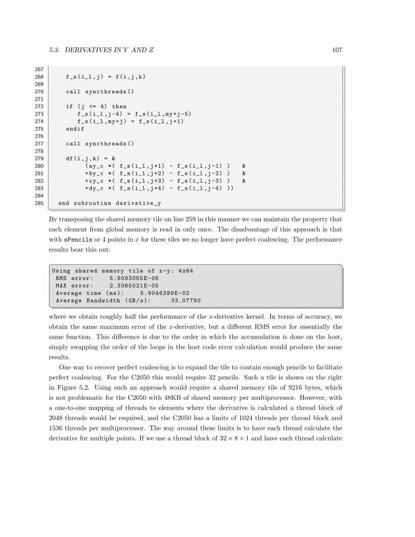
5.3. DERIVATIVES IN Y AND Z 107
267
268 f_s(i_l ,j) = f(i,j,k)
269
270 call syncthreads ()
271
272 if (j <= 4) then
273 f_s(i_l ,j-4) = f_s(i_l ,my+j-5)
274 f_s(i_l ,my+j) = f_s(i_l ,j+1)
275 endif
276
277 call syncthreads ()
278
279 df(i,j,k) = &
280 (ay_c *( f_s(i_l ,j+1) - f_s(i_l ,j-1) ) &
281 +by_c *( f_s(i_l ,j+2) - f_s(i_l ,j-2) ) &
282 +cy_c *( f_s(i_l ,j+3) - f_s(i_l ,j-3) ) &
283 +dy_c *( f_s(i_l ,j+4) - f_s(i_l ,j-4) ))
284
285 end subroutine derivative_y
By transposing the shared memory tile on line 259 in this manner we can maintain the property that
each element from global memory is read in only once. The disadvantage of this approach is that
with sPencils or 4 points in x for these tiles we no longer have perfect coalescing. The performance
results bear this out:� �Using shared memory tile of x-y: 4x64
RMS error: 5.8093055E-06
MAX error: 2.3365021E-05
Average time (ms): 5.9046399E-02
Average Bandwidth (GB/s): 33.07780�where we obtain roughly half the performance of the x-derivative kernel. In terms of accuracy, we
obtain the same maximum error of the x-derivative, but a different RMS error for essentially the
same function. This difference is due to the order in which the accumulation is done on the host,
simply swapping the order of the loops in the host code error calculation would produce the same
results.
One way to recover perfect coalescing is to expand the tile to contain enough pencils to facilitate
perfect coalescing. For the C2050 this would require 32 pencils. Such a tile is shown on the right
in Figure 5.2. Using such an approach would require a shared memory tile of 9216 bytes, which
is not problematic for the C2050 with 48KB of shared memory per multiprocessor. However, with
a one-to-one mapping of threads to elements where the derivative is calculated a thread block of
2048 threads would be required, and the C2050 has a limits of 1024 threads per thread block and
1536 threads per multiprocessor. The way around these limits is to have each thread calculate the
derivative for multiple points. If we use a thread block of 32× 8× 1 and have each thread calculate
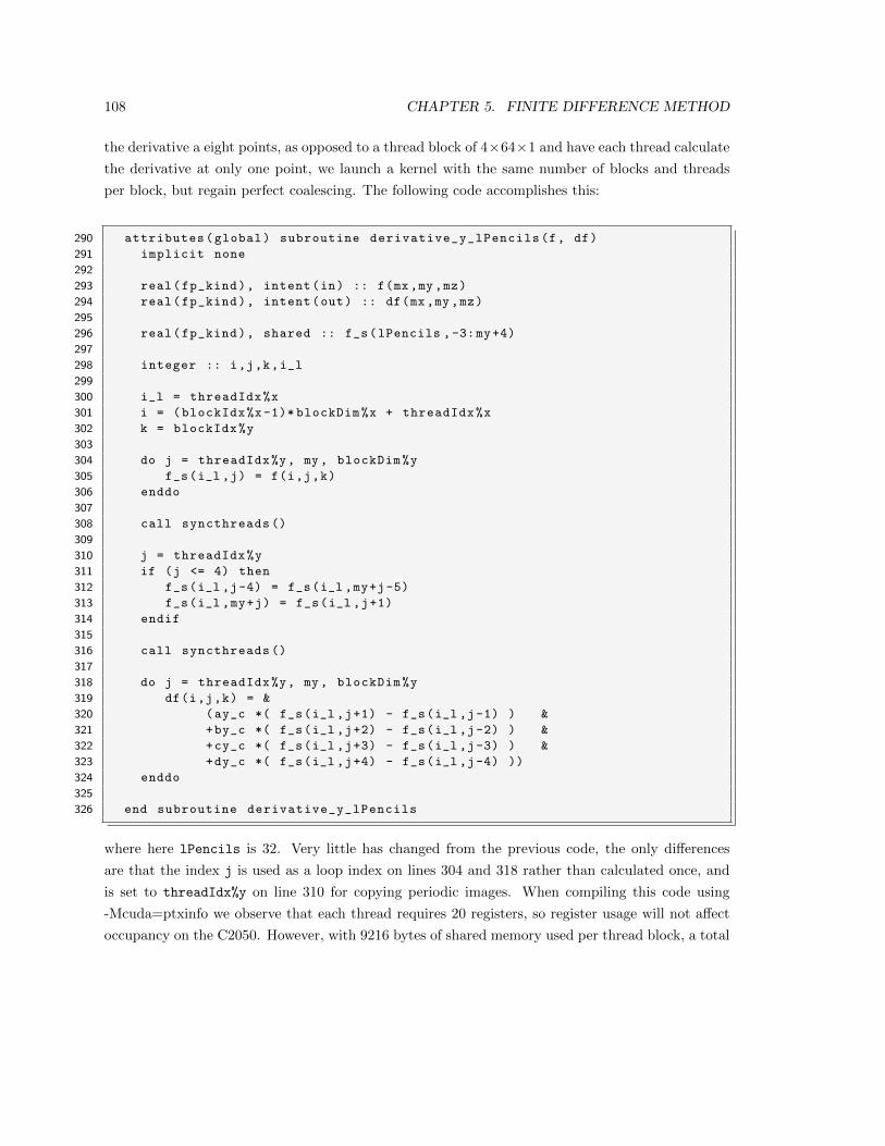
108 CHAPTER 5. FINITE DIFFERENCE METHOD
the derivative a eight points, as opposed to a thread block of 4×64×1 and have each thread calculate
the derivative at only one point, we launch a kernel with the same number of blocks and threads
per block, but regain perfect coalescing. The following code accomplishes this:
290 attributes(global) subroutine derivative_y_lPencils(f, df)
291 implicit none
292
293 real(fp_kind), intent(in) :: f(mx,my,mz)
294 real(fp_kind), intent(out) :: df(mx,my,mz)
295
296 real(fp_kind), shared :: f_s(lPencils ,-3:my+4)
297
298 integer :: i,j,k,i_l
299
300 i_l = threadIdx%x
301 i = (blockIdx%x-1)* blockDim%x + threadIdx%x
302 k = blockIdx%y
303
304 do j = threadIdx%y, my, blockDim%y
305 f_s(i_l ,j) = f(i,j,k)
306 enddo
307
308 call syncthreads ()
309
310 j = threadIdx%y
311 if (j <= 4) then
312 f_s(i_l ,j-4) = f_s(i_l ,my+j-5)
313 f_s(i_l ,my+j) = f_s(i_l ,j+1)
314 endif
315
316 call syncthreads ()
317
318 do j = threadIdx%y, my, blockDim%y
319 df(i,j,k) = &
320 (ay_c *( f_s(i_l ,j+1) - f_s(i_l ,j-1) ) &
321 +by_c *( f_s(i_l ,j+2) - f_s(i_l ,j-2) ) &
322 +cy_c *( f_s(i_l ,j+3) - f_s(i_l ,j-3) ) &
323 +dy_c *( f_s(i_l ,j+4) - f_s(i_l ,j-4) ))
324 enddo
325
326 end subroutine derivative_y_lPencils
where here lPencils is 32. Very little has changed from the previous code, the only differences
are that the index j is used as a loop index on lines 304 and 318 rather than calculated once, and
is set to threadIdx%y on line 310 for copying periodic images. When compiling this code using
-Mcuda=ptxinfo we observe that each thread requires 20 registers, so register usage will not affect
occupancy on the C2050. However, with 9216 bytes of shared memory used per thread block, a total
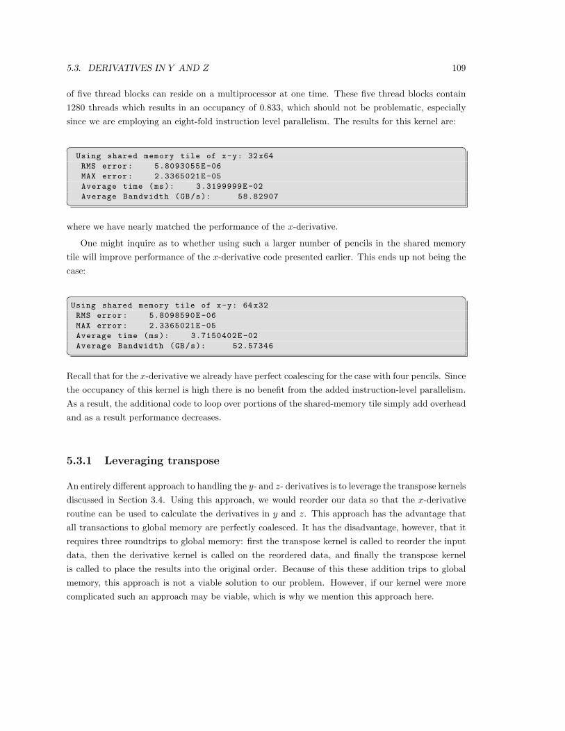
5.3. DERIVATIVES IN Y AND Z 109
of five thread blocks can reside on a multiprocessor at one time. These five thread blocks contain
1280 threads which results in an occupancy of 0.833, which should not be problematic, especially
since we are employing an eight-fold instruction level parallelism. The results for this kernel are:
� �Using shared memory tile of x-y: 32x64
RMS error: 5.8093055E-06
MAX error: 2.3365021E-05
Average time (ms): 3.3199999E-02
Average Bandwidth (GB/s): 58.82907�where we have nearly matched the performance of the x-derivative.
One might inquire as to whether using such a larger number of pencils in the shared memory
tile will improve performance of the x-derivative code presented earlier. This ends up not being the
case:
� �Using shared memory tile of x-y: 64x32
RMS error: 5.8098590E-06
MAX error: 2.3365021E-05
Average time (ms): 3.7150402E-02
Average Bandwidth (GB/s): 52.57346�Recall that for the x-derivative we already have perfect coalescing for the case with four pencils. Since
the occupancy of this kernel is high there is no benefit from the added instruction-level parallelism.
As a result, the additional code to loop over portions of the shared-memory tile simply add overhead
and as a result performance decreases.
5.3.1 Leveraging transpose
An entirely different approach to handling the y- and z- derivatives is to leverage the transpose kernels
discussed in Section 3.4. Using this approach, we would reorder our data so that the x-derivative
routine can be used to calculate the derivatives in y and z. This approach has the advantage that
all transactions to global memory are perfectly coalesced. It has the disadvantage, however, that it
requires three roundtrips to global memory: first the transpose kernel is called to reorder the input
data, then the derivative kernel is called on the reordered data, and finally the transpose kernel
is called to place the results into the original order. Because of this these addition trips to global
memory, this approach is not a viable solution to our problem. However, if our kernel were more
complicated such an approach may be viable, which is why we mention this approach here.
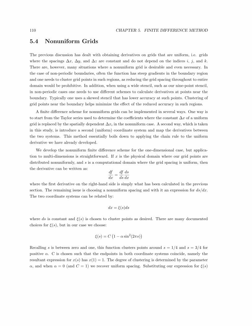
110 CHAPTER 5. FINITE DIFFERENCE METHOD
5.4 Nonuniform Grids
The previous discussion has dealt with obtaining derivatives on grids that are uniform, i.e. grids
where the spacings ∆x, ∆y, and ∆z are constant and do not depend on the indices i, j, and k.
There are, however, many situations where a nonuniform grid is desirable and even necessary. In
the case of non-periodic boundaries, often the function has steep gradients in the boundary region
and one needs to cluster grid points in such regions, as reducing the grid spacing throughout to entire
domain would be prohibitive. In addition, when using a wide stencil, such as our nine-point stencil,
in non-periodic cases one needs to use different schemes to calculate derivatives at points near the
boundary. Typically one uses a skewed stencil that has lower accuracy at such points. Clustering of
grid points near the boundary helps minimize the effect of the reduced accuracy in such regions.
A finite difference scheme for nonuniform grids can be implemented in several ways. One way is
to start from the Taylor series used to determine the coefficients where the constant ∆x of a uniform
grid is replaced by the spatially dependent ∆xi in the nonuniform case. A second way, which is taken
in this study, is introduce a second (uniform) coordinate system and map the derivatives between
the two systems. This method essentially boils down to applying the chain rule to the uniform
derivative we have already developed.
We develop the nonuniform finite difference scheme for the one-dimensional case, but applica-
tion to multi-dimensions is straightforward. If x is the physical domain where our grid points are
distributed nonuniformly, and s is a computational domain where the grid spacing is uniform, then
the derivative can be written as:df
dx=df
ds
ds
dx
where the first derivative on the right-hand side is simply what has been calculated in the previous
section. The remaining issue is choosing a nonuniform spacing and with it an expression for ds/dx.
The two coordinate systems can be related by:
dx = ξ(s)ds
where ds is constant and ξ(s) is chosen to cluster points as desired. There are many documented
choices for ξ(s), but in our case we choose:
ξ(s) = C(1− α sin2(2πs)
)Recalling s is between zero and one, this function clusters points around s = 1/4 and s = 3/4 for
positive α. C is chosen such that the endpoints in both coordinate systems coincide, namely the
resultant expression for x(s) has x(1) = 1. The degree of clustering is determined by the parameter
α, and when α = 0 (and C = 1) we recover uniform spacing. Substituting our expression for ξ(s)
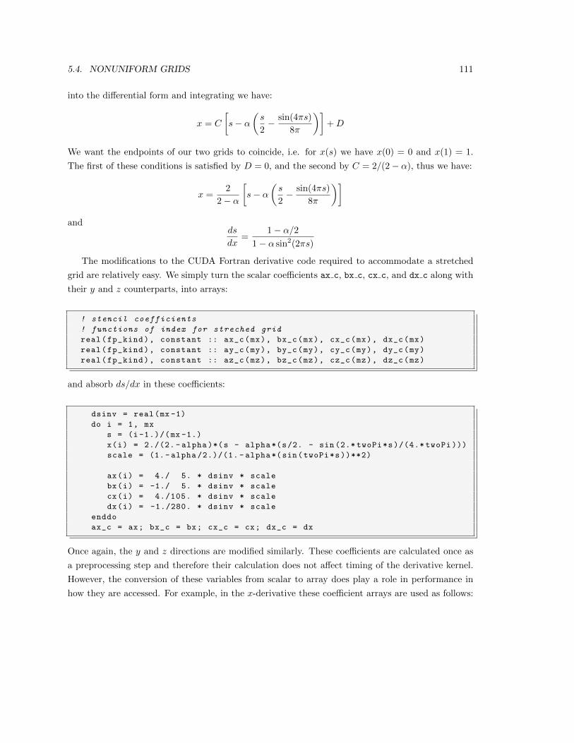
5.4. NONUNIFORM GRIDS 111
into the differential form and integrating we have:
x = C
[s− α
(s
2− sin(4πs)
8π
)]+D
We want the endpoints of our two grids to coincide, i.e. for x(s) we have x(0) = 0 and x(1) = 1.
The first of these conditions is satisfied by D = 0, and the second by C = 2/(2− α), thus we have:
x =2
2− α
[s− α
(s
2− sin(4πs)
8π
)]and
ds
dx=
1− α/21− α sin2(2πs)
The modifications to the CUDA Fortran derivative code required to accommodate a stretched
grid are relatively easy. We simply turn the scalar coefficients ax c, bx c, cx c, and dx c along with
their y and z counterparts, into arrays:
! stencil coefficients
! functions of index for streched grid
real(fp_kind), constant :: ax_c(mx), bx_c(mx), cx_c(mx), dx_c(mx)
real(fp_kind), constant :: ay_c(my), by_c(my), cy_c(my), dy_c(my)
real(fp_kind), constant :: az_c(mz), bz_c(mz), cz_c(mz), dz_c(mz)
and absorb ds/dx in these coefficients:
dsinv = real(mx -1)
do i = 1, mx
s = (i -1.)/(mx -1.)
x(i) = 2./(2. - alpha )*(s - alpha*(s/2. - sin (2.* twoPi*s)/(4.* twoPi )))
scale = (1.- alpha /2.)/(1. - alpha*(sin(twoPi*s))**2)
ax(i) = 4./ 5. * dsinv * scale
bx(i) = -1./ 5. * dsinv * scale
cx(i) = 4./105. * dsinv * scale
dx(i) = -1./280. * dsinv * scale
enddo
ax_c = ax; bx_c = bx; cx_c = cx; dx_c = dx
Once again, the y and z directions are modified similarly. These coefficients are calculated once as
a preprocessing step and therefore their calculation does not affect timing of the derivative kernel.
However, the conversion of these variables from scalar to array does play a role in performance in
how they are accessed. For example, in the x-derivative these coefficient arrays are used as follows:
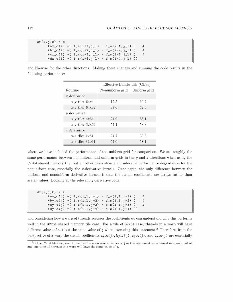
112 CHAPTER 5. FINITE DIFFERENCE METHOD
df(i,j,k) = &
(ax_c(i) *( f_s(i+1,j_l) - f_s(i-1,j_l) ) &
+bx_c(i) *( f_s(i+2,j_l) - f_s(i-2,j_l) ) &
+cx_c(i) *( f_s(i+3,j_l) - f_s(i-3,j_l) ) &
+dx_c(i) *( f_s(i+4,j_l) - f_s(i-4,j_l) ))
and likewise for the other directions. Making these changes and running the code results in the
following performance:
Effective Bandwidth (GB/s)
Routine Nonuniform grid Uniform grid
x derivative
x-y tile: 64x4 12.5 60.2
x-y tile: 64x32 37.6 52.6
y derivative
x-y tile: 4x64 24.9 33.1
x-y tile: 32x64 57.1 58.8
z derivative
x-z tile: 4x64 24.7 33.3
x-z tile: 32x64 57.0 58.1
where we have included the performance of the uniform grid for comparison. We see roughly the
same performance between nonuniform and uniform grids in the y and z directions when using the
32x64 shared memory tile, but all other cases show a considerable performance degradation for the
nonuniform case, especially the x-derivative kernels. Once again, the only difference between the
uniform and nonuniform derivative kernels is that the stencil coefficients are arrays rather than
scalar values. Looking at the relevant y derivative code:
df(i,j,k) = &
(ay_c(j) *( f_s(i_l ,j+1) - f_s(i_l ,j-1) ) &
+by_c(j) *( f_s(i_l ,j+2) - f_s(i_l ,j-2) ) &
+cy_c(j) *( f_s(i_l ,j+3) - f_s(i_l ,j-3) ) &
+dy_c(j) *( f_s(i_l ,j+4) - f_s(i_l ,j-4) ))
and considering how a warp of threads accesses the coefficients we can understand why this performs
well in the 32x64 shared memory tile case. For a tile of 32x64 case, threads in a warp will have
different values of i l but the same value of j when executing this statement.2 Therefore, from the
perspective of a warp the stencil coefficients ay c(j), by c(j), cy c(j), and dy c(j) are essentially
2In the 32x64 tile case, each thread will take on several values of j as this statement is contained in a loop, but atany one time all threads in a warp will have the same value of j.
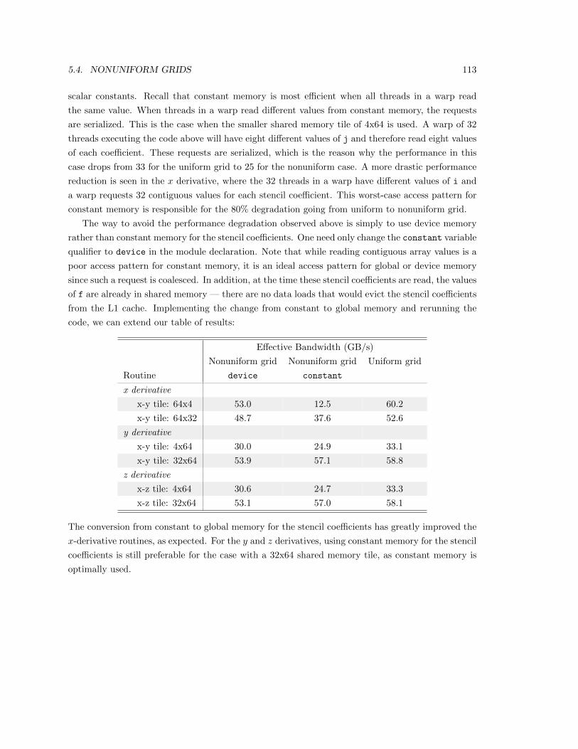
5.4. NONUNIFORM GRIDS 113
scalar constants. Recall that constant memory is most efficient when all threads in a warp read
the same value. When threads in a warp read different values from constant memory, the requests
are serialized. This is the case when the smaller shared memory tile of 4x64 is used. A warp of 32
threads executing the code above will have eight different values of j and therefore read eight values
of each coefficient. These requests are serialized, which is the reason why the performance in this
case drops from 33 for the uniform grid to 25 for the nonuniform case. A more drastic performance
reduction is seen in the x derivative, where the 32 threads in a warp have different values of i and
a warp requests 32 contiguous values for each stencil coefficient. This worst-case access pattern for
constant memory is responsible for the 80% degradation going from uniform to nonuniform grid.
The way to avoid the performance degradation observed above is simply to use device memory
rather than constant memory for the stencil coefficients. One need only change the constant variable
qualifier to device in the module declaration. Note that while reading contiguous array values is a
poor access pattern for constant memory, it is an ideal access pattern for global or device memory
since such a request is coalesced. In addition, at the time these stencil coefficients are read, the values
of f are already in shared memory — there are no data loads that would evict the stencil coefficients
from the L1 cache. Implementing the change from constant to global memory and rerunning the
code, we can extend our table of results:
Effective Bandwidth (GB/s)
Nonuniform grid Nonuniform grid Uniform grid
Routine device constant
x derivative
x-y tile: 64x4 53.0 12.5 60.2
x-y tile: 64x32 48.7 37.6 52.6
y derivative
x-y tile: 4x64 30.0 24.9 33.1
x-y tile: 32x64 53.9 57.1 58.8
z derivative
x-z tile: 4x64 30.6 24.7 33.3
x-z tile: 32x64 53.1 57.0 58.1
The conversion from constant to global memory for the stencil coefficients has greatly improved the
x-derivative routines, as expected. For the y and z derivatives, using constant memory for the stencil
coefficients is still preferable for the case with a 32x64 shared memory tile, as constant memory is
optimally used.

114 CHAPTER 5. FINITE DIFFERENCE METHOD

Part III
Appendices
115

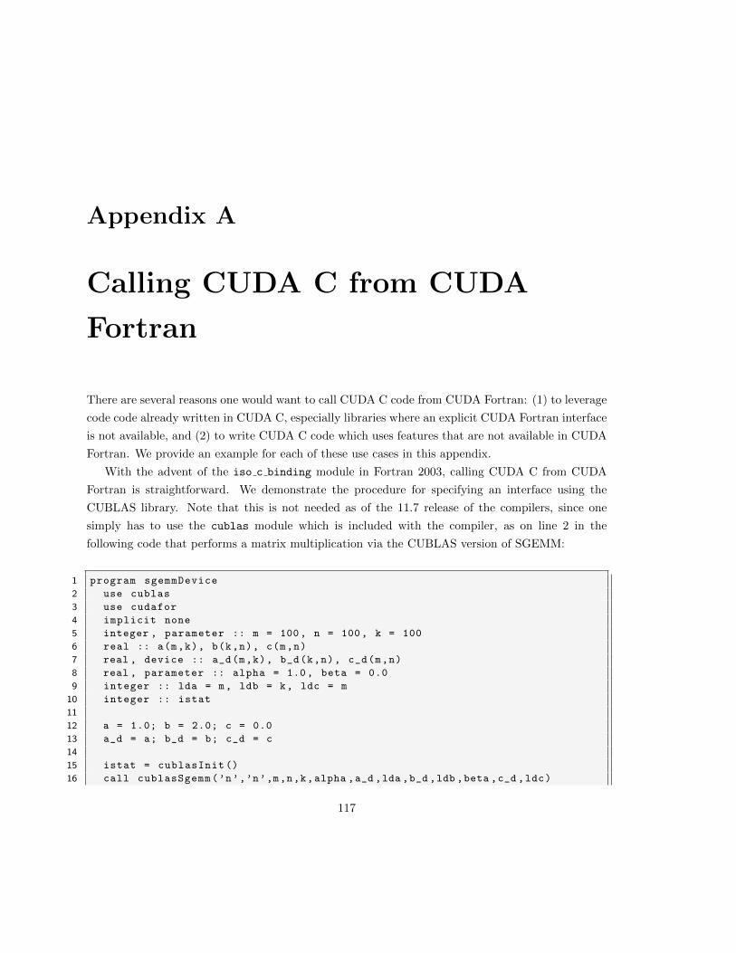
Appendix A
Calling CUDA C from CUDA
Fortran
There are several reasons one would want to call CUDA C code from CUDA Fortran: (1) to leverage
code code already written in CUDA C, especially libraries where an explicit CUDA Fortran interface
is not available, and (2) to write CUDA C code which uses features that are not available in CUDA
Fortran. We provide an example for each of these use cases in this appendix.
With the advent of the iso c binding module in Fortran 2003, calling CUDA C from CUDA
Fortran is straightforward. We demonstrate the procedure for specifying an interface using the
CUBLAS library. Note that this is not needed as of the 11.7 release of the compilers, since one
simply has to use the cublas module which is included with the compiler, as on line 2 in the
following code that performs a matrix multiplication via the CUBLAS version of SGEMM:
1 program sgemmDevice
2 use cublas
3 use cudafor
4 implicit none
5 integer , parameter :: m = 100, n = 100, k = 100
6 real :: a(m,k), b(k,n), c(m,n)
7 real , device :: a_d(m,k), b_d(k,n), c_d(m,n)
8 real , parameter :: alpha = 1.0, beta = 0.0
9 integer :: lda = m, ldb = k, ldc = m
10 integer :: istat
11
12 a = 1.0; b = 2.0; c = 0.0
13 a_d = a; b_d = b; c_d = c
14
15 istat = cublasInit ()
16 call cublasSgemm(’n’,’n’,m,n,k,alpha ,a_d ,lda ,b_d ,ldb ,beta ,c_d ,ldc)
117

118 APPENDIX A. CALLING CUDA C FROM CUDA FORTRAN
17
18 c = c_d
19 write (*,*) ’Max error =’, maxval(c-k*2.0)
20
21 end program sgemmDevice
Here the cublas module defines the interfaces for all the CUBLAS routines, including cublasInit()
and cublasSgemm(). Prior to the cublas module introduced in the 11.7 compilers, one had to
explicitly interface with the C routines in the CUBLAS library, as in the user-defined cublas m
module below:
1 module cublas_m
2 interface cublasInit
3 integer function cublasInit () bind(C,name=’cublasInit ’)
4 end function cublasInit
5 end interface
6
7 interface cublasSgemm
8 subroutine cublasSgemm(cta ,ctb ,m,n,k,alpha ,A,lda ,B,ldb ,beta ,c,ldc) &
9 bind(C,name=’cublasSgemm ’)
10 use iso_c_binding
11 character (1,c_char), value :: cta , ctb
12 integer(c_int), value :: k, m, n, lda , ldb , ldc
13 real(c_float), value :: alpha , beta
14 real(c_float), device :: A(lda ,*), B(ldb ,*), C(ldc ,*)
15 end subroutine cublasSgemm
16 end interface cublasSgemm
17 end module cublas_m
18
19
20 program sgemmDevice
21 use cublas_m
22 use cudafor
23 implicit none
24 integer , parameter :: m = 100, n = 100, k = 100
25 real :: a(m,k), b(k,n), c(m,n)
26 real , device :: a_d(m,k), b_d(k,n), c_d(m,n)
27 real , parameter :: alpha = 1.0, beta = 0.0
28 integer :: lda = m, ldb = k, ldc = m
29 integer :: istat
30
31 a = 1.0; b = 2.0; c = 0.0
32 a_d = a; b_d = b; c_d = c
33
34 istat = cublasInit ()
35 call cublasSgemm(’n’,’n’,m,n,k,alpha ,a_d ,lda ,b_d ,ldb ,beta ,c_d ,ldc)
36
37 c = c_d
38 write (*,*) ’Max error =’, maxval(c-k*2.0)
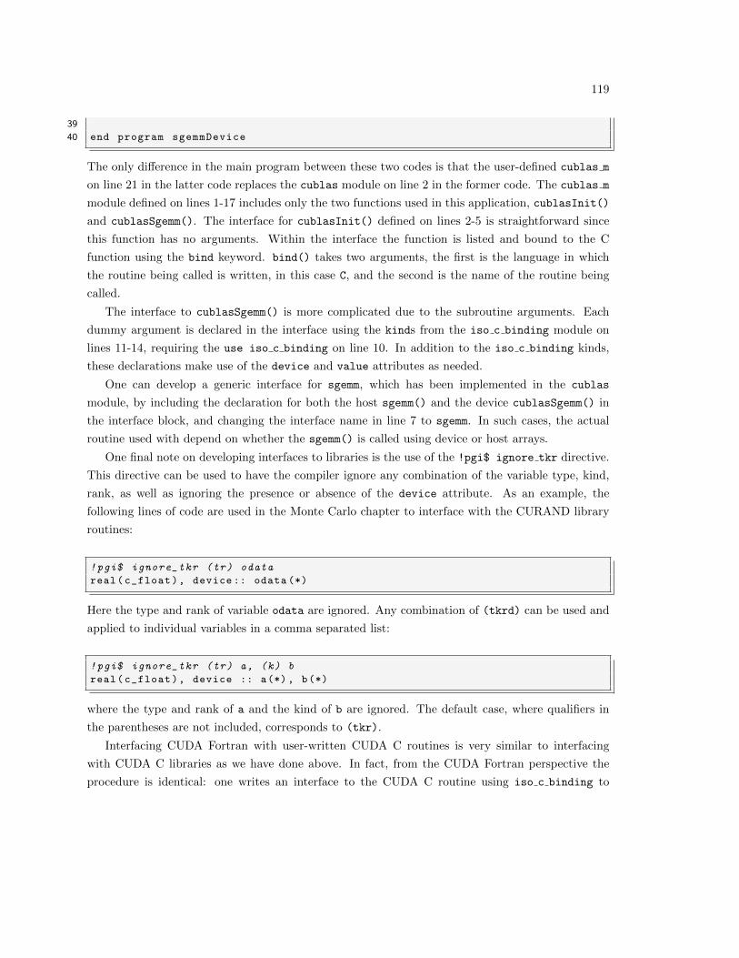
119
39
40 end program sgemmDevice
The only difference in the main program between these two codes is that the user-defined cublas m
on line 21 in the latter code replaces the cublas module on line 2 in the former code. The cublas m
module defined on lines 1-17 includes only the two functions used in this application, cublasInit()
and cublasSgemm(). The interface for cublasInit() defined on lines 2-5 is straightforward since
this function has no arguments. Within the interface the function is listed and bound to the C
function using the bind keyword. bind() takes two arguments, the first is the language in which
the routine being called is written, in this case C, and the second is the name of the routine being
called.
The interface to cublasSgemm() is more complicated due to the subroutine arguments. Each
dummy argument is declared in the interface using the kinds from the iso c binding module on
lines 11-14, requiring the use iso c binding on line 10. In addition to the iso c binding kinds,
these declarations make use of the device and value attributes as needed.
One can develop a generic interface for sgemm, which has been implemented in the cublas
module, by including the declaration for both the host sgemm() and the device cublasSgemm() in
the interface block, and changing the interface name in line 7 to sgemm. In such cases, the actual
routine used with depend on whether the sgemm() is called using device or host arrays.
One final note on developing interfaces to libraries is the use of the !pgi$ ignore tkr directive.
This directive can be used to have the compiler ignore any combination of the variable type, kind,
rank, as well as ignoring the presence or absence of the device attribute. As an example, the
following lines of code are used in the Monte Carlo chapter to interface with the CURAND library
routines:
!pgi$ ignore_tkr (tr) odata
real(c_float), device :: odata (*)
Here the type and rank of variable odata are ignored. Any combination of (tkrd) can be used and
applied to individual variables in a comma separated list:
!pgi$ ignore_tkr (tr) a, (k) b
real(c_float), device :: a(*), b(*)
where the type and rank of a and the kind of b are ignored. The default case, where qualifiers in
the parentheses are not included, corresponds to (tkr).
Interfacing CUDA Fortran with user-written CUDA C routines is very similar to interfacing
with CUDA C libraries as we have done above. In fact, from the CUDA Fortran perspective the
procedure is identical: one writes an interface to the CUDA C routine using iso c binding to
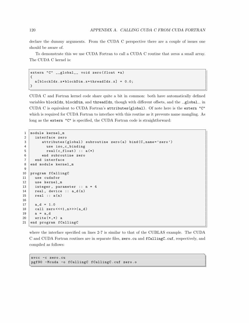
120 APPENDIX A. CALLING CUDA C FROM CUDA FORTRAN
declare the dummy arguments. From the CUDA C perspective there are a couple of issues one
should be aware of.
To demonstrate this we use CUDA Fortran to call a CUDA C routine that zeros a small array.
The CUDA C kernel is:
extern "C" __global__ void zero(float *a)
{
a[blockIdx.x*blockDim.x+threadIdx.x] = 0.0;
}
CUDA C and Fortran kernel code share quite a bit in common: both have automatically defined
variables blockIdx, blockDim, and threadIdx, though with different offsets, and the global in
CUDA C is equivalent to CUDA Fortran’s attributes(global). Of note here is the extern "C"
which is required for CUDA Fortran to interface with this routine as it prevents name mangling. As
long as the extern "C" is specified, the CUDA Fortran code is straightforward:
1 module kernel_m
2 interface zero
3 attributes(global) subroutine zero(a) bind(C,name=’zero’)
4 use iso_c_binding
5 real(c_float) :: a(*)
6 end subroutine zero
7 end interface
8 end module kernel_m
9
10 program fCallingC
11 use cudafor
12 use kernel_m
13 integer , parameter :: n = 4
14 real , device :: a_d(n)
15 real :: a(n)
16
17 a_d = 1.0
18 call zero <<<1,n>>>(a_d)
19 a = a_d
20 write (*,*) a
21 end program fCallingC
where the interface specified on lines 2-7 is similar to that of the CUBLAS example. The CUDA
C and CUDA Fortran routines are in separate files, zero.cu and fCallingC.cuf, respectively, and
compiled as follows:� �nvcc -c zero.cu
pgf90 -Mcuda -o fCallingC fCallingC.cuf zero.o�

121
where the nvcc compiler is used for compiling zero.cu.

122 APPENDIX A. CALLING CUDA C FROM CUDA FORTRAN
Appendix B
Source Code
CUDA Fortran source code that was deemed to long to include in its entirety in earlier chapters is
listed in this appendix. Each section in this appendix contains all the relevant code, both host and
device code, for the particular application.
123
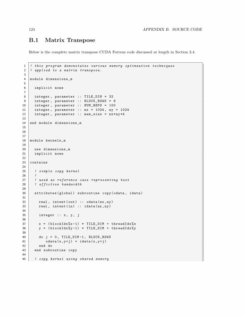
124 APPENDIX B. SOURCE CODE
B.1 Matrix Transpose
Below is the complete matrix transpose CUDA Fortran code discussed at length in Section 3.4.
1 ! this program demonstates various memory optimzation techniques
2 ! applied to a matrix transpose.
3
4 module dimensions_m
5
6 implicit none
7
8 integer , parameter :: TILE_DIM = 32
9 integer , parameter :: BLOCK_ROWS = 8
10 integer , parameter :: NUM_REPS = 100
11 integer , parameter :: nx = 1024, ny = 1024
12 integer , parameter :: mem_size = nx*ny*4
13
14 end module dimensions_m
15
16
17
18 module kernels_m
19
20 use dimensions_m
21 implicit none
22
23 contains
24
25 ! simple copy kernel
26 !
27 ! used as reference case representing best
28 ! effictive bandwidth
29
30 attributes(global) subroutine copy(odata , idata)
31
32 real , intent(out) :: odata(nx,ny)
33 real , intent(in) :: idata(nx,ny)
34
35 integer :: x, y, j
36
37 x = (blockIdx%x-1) * TILE_DIM + threadIdx%x
38 y = (blockIdx%y-1) * TILE_DIM + threadIdx%y
39
40 do j = 0, TILE_DIM -1, BLOCK_ROWS
41 odata(x,y+j) = idata(x,y+j)
42 end do
43 end subroutine copy
44
45 ! copy kernel using shared memory
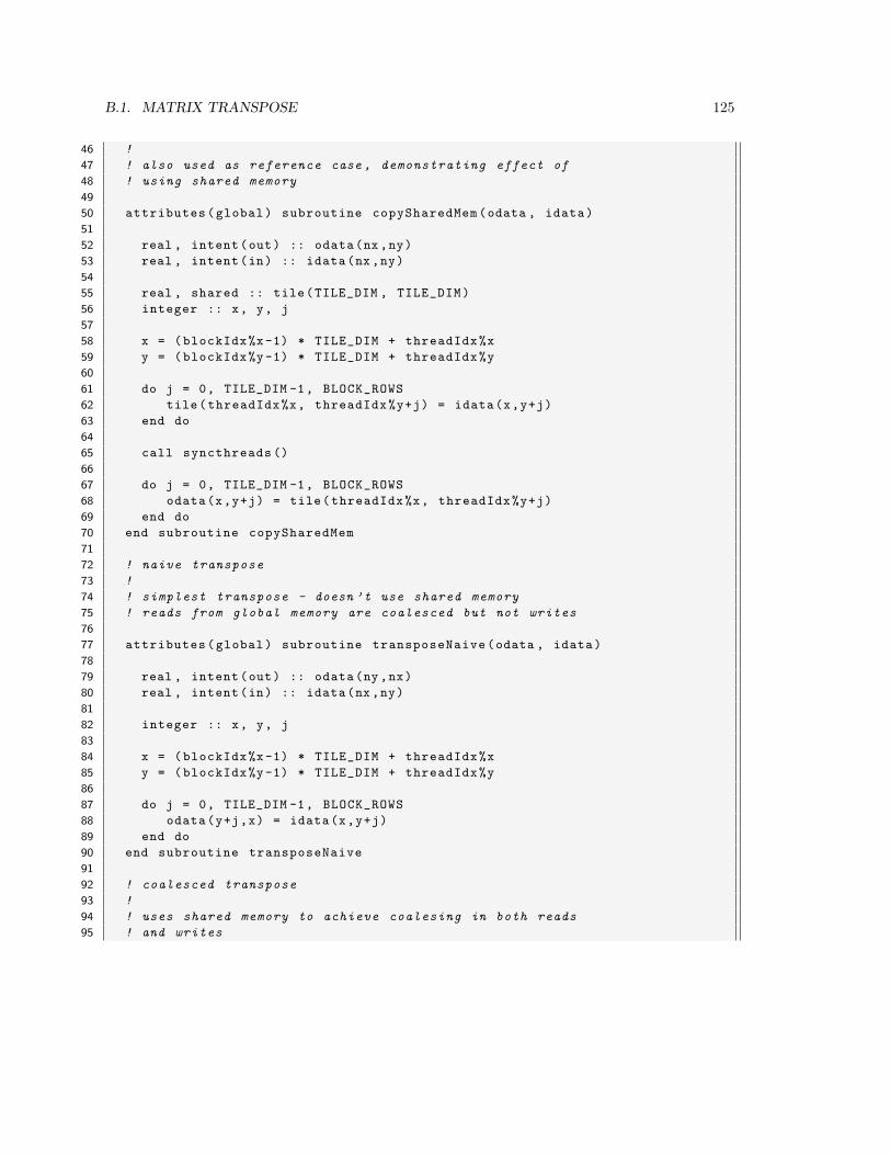
B.1. MATRIX TRANSPOSE 125
46 !
47 ! also used as reference case , demonstrating effect of
48 ! using shared memory
49
50 attributes(global) subroutine copySharedMem(odata , idata)
51
52 real , intent(out) :: odata(nx,ny)
53 real , intent(in) :: idata(nx,ny)
54
55 real , shared :: tile(TILE_DIM , TILE_DIM)
56 integer :: x, y, j
57
58 x = (blockIdx%x-1) * TILE_DIM + threadIdx%x
59 y = (blockIdx%y-1) * TILE_DIM + threadIdx%y
60
61 do j = 0, TILE_DIM -1, BLOCK_ROWS
62 tile(threadIdx%x, threadIdx%y+j) = idata(x,y+j)
63 end do
64
65 call syncthreads ()
66
67 do j = 0, TILE_DIM -1, BLOCK_ROWS
68 odata(x,y+j) = tile(threadIdx%x, threadIdx%y+j)
69 end do
70 end subroutine copySharedMem
71
72 ! naive transpose
73 !
74 ! simplest transpose - doesn ’t use shared memory
75 ! reads from global memory are coalesced but not writes
76
77 attributes(global) subroutine transposeNaive(odata , idata)
78
79 real , intent(out) :: odata(ny,nx)
80 real , intent(in) :: idata(nx,ny)
81
82 integer :: x, y, j
83
84 x = (blockIdx%x-1) * TILE_DIM + threadIdx%x
85 y = (blockIdx%y-1) * TILE_DIM + threadIdx%y
86
87 do j = 0, TILE_DIM -1, BLOCK_ROWS
88 odata(y+j,x) = idata(x,y+j)
89 end do
90 end subroutine transposeNaive
91
92 ! coalesced transpose
93 !
94 ! uses shared memory to achieve coalesing in both reads
95 ! and writes
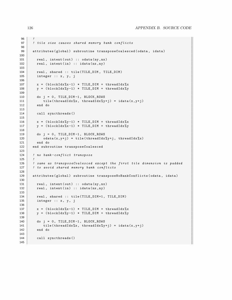
126 APPENDIX B. SOURCE CODE
96 !
97 ! tile size causes shared memory bank conflicts
98
99 attributes(global) subroutine transposeCoalesced(odata , idata)
100
101 real , intent(out) :: odata(ny,nx)
102 real , intent(in) :: idata(nx,ny)
103
104 real , shared :: tile(TILE_DIM , TILE_DIM)
105 integer :: x, y, j
106
107 x = (blockIdx%x-1) * TILE_DIM + threadIdx%x
108 y = (blockIdx%y-1) * TILE_DIM + threadIdx%y
109
110 do j = 0, TILE_DIM -1, BLOCK_ROWS
111 tile(threadIdx%x, threadIdx%y+j) = idata(x,y+j)
112 end do
113
114 call syncthreads ()
115
116 x = (blockIdx%y-1) * TILE_DIM + threadIdx%x
117 y = (blockIdx%x-1) * TILE_DIM + threadIdx%y
118
119 do j = 0, TILE_DIM -1, BLOCK_ROWS
120 odata(x,y+j) = tile(threadIdx%y+j, threadIdx%x)
121 end do
122 end subroutine transposeCoalesced
123
124 ! no bank -conflict transpose
125 !
126 ! same as transposeCoalesced except the first tile dimension is padded
127 ! to avoid shared memory bank conflicts
128
129 attributes(global) subroutine transposeNoBankConflicts(odata , idata)
130
131 real , intent(out) :: odata(ny,nx)
132 real , intent(in) :: idata(nx,ny)
133
134 real , shared :: tile(TILE_DIM+1, TILE_DIM)
135 integer :: x, y, j
136
137 x = (blockIdx%x-1) * TILE_DIM + threadIdx%x
138 y = (blockIdx%y-1) * TILE_DIM + threadIdx%y
139
140 do j = 0, TILE_DIM -1, BLOCK_ROWS
141 tile(threadIdx%x, threadIdx%y+j) = idata(x,y+j)
142 end do
143
144 call syncthreads ()
145

B.1. MATRIX TRANSPOSE 127
146 x = (blockIdx%y-1) * TILE_DIM + threadIdx%x
147 y = (blockIdx%x-1) * TILE_DIM + threadIdx%y
148
149 do j = 0, TILE_DIM -1, BLOCK_ROWS
150 odata(x,y+j) = tile(threadIdx%y+j, threadIdx%x)
151 end do
152 end subroutine transposeNoBankConflicts
153
154 ! Diagonal reordering
155 !
156 ! This version should be used on cards of compute capability 1.3
157 ! to avoid partition camping. It essentially reschedules the
158 ! order in which blocks are executed so requests for global
159 ! memory access by active blocks are spread evenly amongst
160 ! partitions
161
162 attributes(global) subroutine transposeDiagonal(odata , idata)
163
164 real , intent(out) :: odata(ny,nx)
165 real , intent(in) :: idata(nx,ny)
166
167 real , shared :: tile(TILE_DIM+1, TILE_DIM)
168 integer :: x, y, j
169 integer :: blockIdx_x , blockIdx_y
170
171 if (nx==ny) then
172 blockIdx_y = blockIdx%x
173 blockIdx_x = mod(blockIdx%x+blockIdx%y-2,gridDim%x)+1
174 else
175 x = blockIdx%x + gridDim%x*( blockIdx%y-1)
176 blockIdx_y = mod(x-1,gridDim%y)+1
177 blockIdx_x = mod((x-1)/ gridDim%y+blockIdx_y -1,gridDim%x)+1
178 endif
179
180 x = (blockIdx_x -1) * TILE_DIM + threadIdx%x
181 y = (blockIdx_y -1) * TILE_DIM + threadIdx%y
182
183 do j = 0, TILE_DIM -1, BLOCK_ROWS
184 tile(threadIdx%x, threadIdx%y+j) = idata(x,y+j)
185 end do
186
187 call syncthreads ()
188
189 x = (blockIdx_y -1) * TILE_DIM + threadIdx%x
190 y = (blockIdx_x -1) * TILE_DIM + threadIdx%y
191
192 do j = 0, TILE_DIM -1, BLOCK_ROWS
193 odata(x,y+j) = tile(threadIdx%y+j, threadIdx%x)
194 end do
195 end subroutine transposeDiagonal
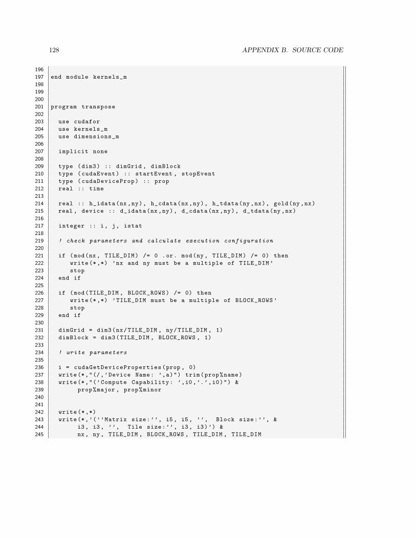
128 APPENDIX B. SOURCE CODE
196
197 end module kernels_m
198
199
200
201 program transpose
202
203 use cudafor
204 use kernels_m
205 use dimensions_m
206
207 implicit none
208
209 type (dim3) :: dimGrid , dimBlock
210 type (cudaEvent) :: startEvent , stopEvent
211 type (cudaDeviceProp) :: prop
212 real :: time
213
214 real :: h_idata(nx,ny), h_cdata(nx,ny), h_tdata(ny,nx), gold(ny,nx)
215 real , device :: d_idata(nx,ny), d_cdata(nx,ny), d_tdata(ny,nx)
216
217 integer :: i, j, istat
218
219 ! check parameters and calculate execution configuration
220
221 if (mod(nx, TILE_DIM) /= 0 .or. mod(ny, TILE_DIM) /= 0) then
222 write (*,*) ’nx and ny must be a multiple of TILE_DIM ’
223 stop
224 end if
225
226 if (mod(TILE_DIM , BLOCK_ROWS) /= 0) then
227 write (*,*) ’TILE_DIM must be a multiple of BLOCK_ROWS ’
228 stop
229 end if
230
231 dimGrid = dim3(nx/TILE_DIM , ny/TILE_DIM , 1)
232 dimBlock = dim3(TILE_DIM , BLOCK_ROWS , 1)
233
234 ! write parameters
235
236 i = cudaGetDeviceProperties(prop , 0)
237 write(*,"(/,’Device Name: ’,a)") trim(prop%name)
238 write(*,"(’Compute Capability: ’,i0 ,’.’,i0)") &
239 prop%major , prop%minor
240
241
242 write (*,*)
243 write(*,’(’’Matrix size:’’, i5 , i5 , ’’, Block size:’’, &
244 i3 , i3 , ’’, Tile size:’’, i3 , i3)’) &
245 nx , ny , TILE_DIM , BLOCK_ROWS , TILE_DIM , TILE_DIM
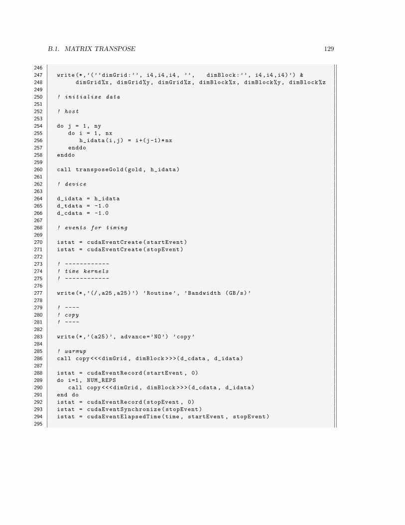
B.1. MATRIX TRANSPOSE 129
246
247 write(*,’(’’dimGrid:’’, i4 ,i4 ,i4 , ’’, dimBlock:’’, i4 ,i4 ,i4)’) &
248 dimGrid%x, dimGrid%y, dimGrid%z, dimBlock%x, dimBlock%y, dimBlock%z
249
250 ! initialize data
251
252 ! host
253
254 do j = 1, ny
255 do i = 1, nx
256 h_idata(i,j) = i+(j-1)*nx
257 enddo
258 enddo
259
260 call transposeGold(gold , h_idata)
261
262 ! device
263
264 d_idata = h_idata
265 d_tdata = -1.0
266 d_cdata = -1.0
267
268 ! events for timing
269
270 istat = cudaEventCreate(startEvent)
271 istat = cudaEventCreate(stopEvent)
272
273 ! ------------
274 ! time kernels
275 ! ------------
276
277 write(*,’(/,a25 ,a25)’) ’Routine ’, ’Bandwidth (GB/s)’
278
279 ! ----
280 ! copy
281 ! ----
282
283 write(*,’(a25)’, advance=’NO’) ’copy’
284
285 ! warmup
286 call copy <<<dimGrid , dimBlock >>>(d_cdata , d_idata)
287
288 istat = cudaEventRecord(startEvent , 0)
289 do i=1, NUM_REPS
290 call copy <<<dimGrid , dimBlock >>>(d_cdata , d_idata)
291 end do
292 istat = cudaEventRecord(stopEvent , 0)
293 istat = cudaEventSynchronize(stopEvent)
294 istat = cudaEventElapsedTime(time , startEvent , stopEvent)
295
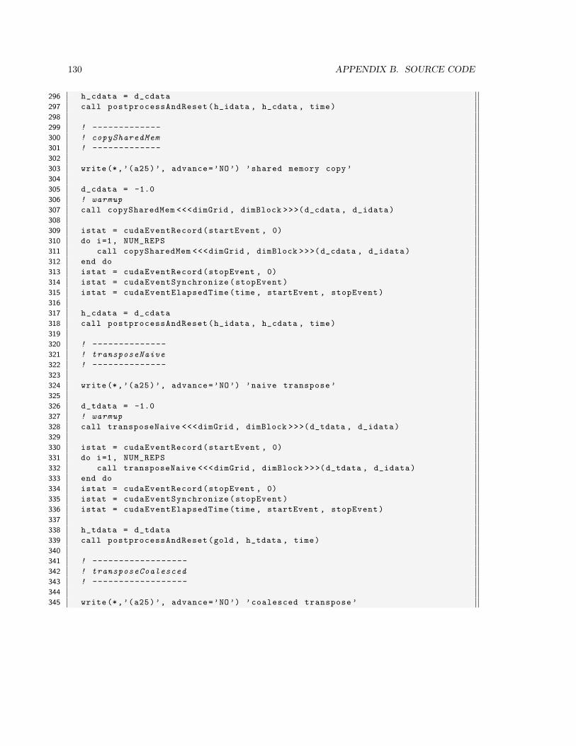
130 APPENDIX B. SOURCE CODE
296 h_cdata = d_cdata
297 call postprocessAndReset(h_idata , h_cdata , time)
298
299 ! -------------
300 ! copySharedMem
301 ! -------------
302
303 write(*,’(a25)’, advance=’NO’) ’shared memory copy’
304
305 d_cdata = -1.0
306 ! warmup
307 call copySharedMem <<<dimGrid , dimBlock >>>(d_cdata , d_idata)
308
309 istat = cudaEventRecord(startEvent , 0)
310 do i=1, NUM_REPS
311 call copySharedMem <<<dimGrid , dimBlock >>>(d_cdata , d_idata)
312 end do
313 istat = cudaEventRecord(stopEvent , 0)
314 istat = cudaEventSynchronize(stopEvent)
315 istat = cudaEventElapsedTime(time , startEvent , stopEvent)
316
317 h_cdata = d_cdata
318 call postprocessAndReset(h_idata , h_cdata , time)
319
320 ! --------------
321 ! transposeNaive
322 ! --------------
323
324 write(*,’(a25)’, advance=’NO’) ’naive transpose ’
325
326 d_tdata = -1.0
327 ! warmup
328 call transposeNaive <<<dimGrid , dimBlock >>>(d_tdata , d_idata)
329
330 istat = cudaEventRecord(startEvent , 0)
331 do i=1, NUM_REPS
332 call transposeNaive <<<dimGrid , dimBlock >>>(d_tdata , d_idata)
333 end do
334 istat = cudaEventRecord(stopEvent , 0)
335 istat = cudaEventSynchronize(stopEvent)
336 istat = cudaEventElapsedTime(time , startEvent , stopEvent)
337
338 h_tdata = d_tdata
339 call postprocessAndReset(gold , h_tdata , time)
340
341 ! ------------------
342 ! transposeCoalesced
343 ! ------------------
344
345 write(*,’(a25)’, advance=’NO’) ’coalesced transpose ’
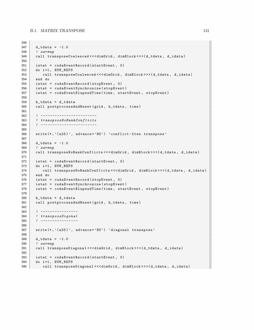
B.1. MATRIX TRANSPOSE 131
346
347 d_tdata = -1.0
348 ! warmup
349 call transposeCoalesced <<<dimGrid , dimBlock >>>(d_tdata , d_idata)
350
351 istat = cudaEventRecord(startEvent , 0)
352 do i=1, NUM_REPS
353 call transposeCoalesced <<<dimGrid , dimBlock >>>(d_tdata , d_idata)
354 end do
355 istat = cudaEventRecord(stopEvent , 0)
356 istat = cudaEventSynchronize(stopEvent)
357 istat = cudaEventElapsedTime(time , startEvent , stopEvent)
358
359 h_tdata = d_tdata
360 call postprocessAndReset(gold , h_tdata , time)
361
362 ! ------------------------
363 ! transposeNoBankConflicts
364 ! ------------------------
365
366 write(*,’(a25)’, advance=’NO’) ’conflict -free transpose ’
367
368 d_tdata = -1.0
369 ! warmup
370 call transposeNoBankConflicts <<<dimGrid , dimBlock >>>(d_tdata , d_idata)
371
372 istat = cudaEventRecord(startEvent , 0)
373 do i=1, NUM_REPS
374 call transposeNoBankConflicts <<<dimGrid , dimBlock >>>(d_tdata , d_idata)
375 end do
376 istat = cudaEventRecord(stopEvent , 0)
377 istat = cudaEventSynchronize(stopEvent)
378 istat = cudaEventElapsedTime(time , startEvent , stopEvent)
379
380 h_tdata = d_tdata
381 call postprocessAndReset(gold , h_tdata , time)
382
383 ! ----------------
384 ! transposeDigonal
385 ! ----------------
386
387 write(*,’(a25)’, advance=’NO’) ’diagonal transpose ’
388
389 d_tdata = -1.0
390 ! warmup
391 call transposeDiagonal <<<dimGrid , dimBlock >>>(d_tdata , d_idata)
392
393 istat = cudaEventRecord(startEvent , 0)
394 do i=1, NUM_REPS
395 call transposeDiagonal <<<dimGrid , dimBlock >>>(d_tdata , d_idata)
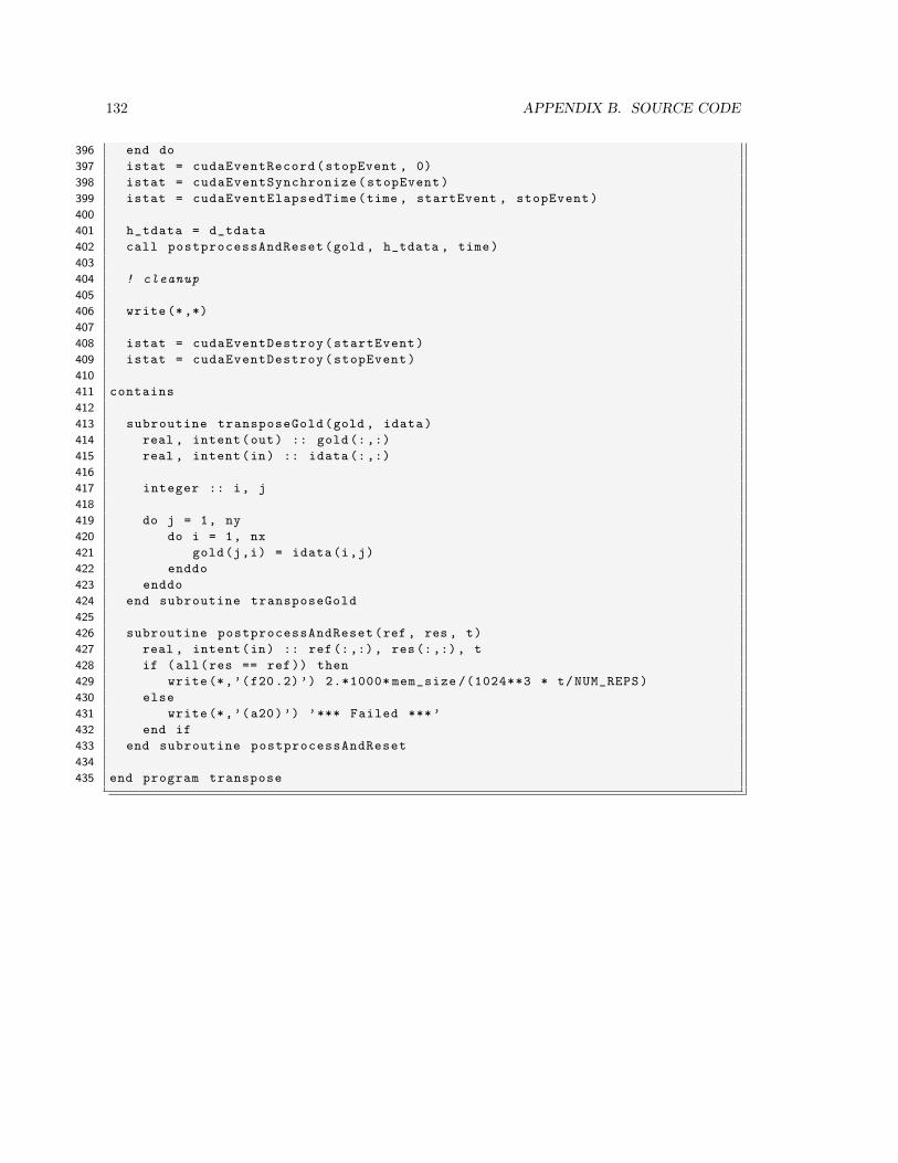
132 APPENDIX B. SOURCE CODE
396 end do
397 istat = cudaEventRecord(stopEvent , 0)
398 istat = cudaEventSynchronize(stopEvent)
399 istat = cudaEventElapsedTime(time , startEvent , stopEvent)
400
401 h_tdata = d_tdata
402 call postprocessAndReset(gold , h_tdata , time)
403
404 ! cleanup
405
406 write (*,*)
407
408 istat = cudaEventDestroy(startEvent)
409 istat = cudaEventDestroy(stopEvent)
410
411 contains
412
413 subroutine transposeGold(gold , idata)
414 real , intent(out) :: gold (:,:)
415 real , intent(in) :: idata (:,:)
416
417 integer :: i, j
418
419 do j = 1, ny
420 do i = 1, nx
421 gold(j,i) = idata(i,j)
422 enddo
423 enddo
424 end subroutine transposeGold
425
426 subroutine postprocessAndReset(ref , res , t)
427 real , intent(in) :: ref(:,:), res(:,:), t
428 if (all(res == ref)) then
429 write(*,’(f20.2)’) 2.*1000* mem_size /(1024**3 * t/NUM_REPS)
430 else
431 write(*,’(a20)’) ’*** Failed ***’
432 end if
433 end subroutine postprocessAndReset
434
435 end program transpose
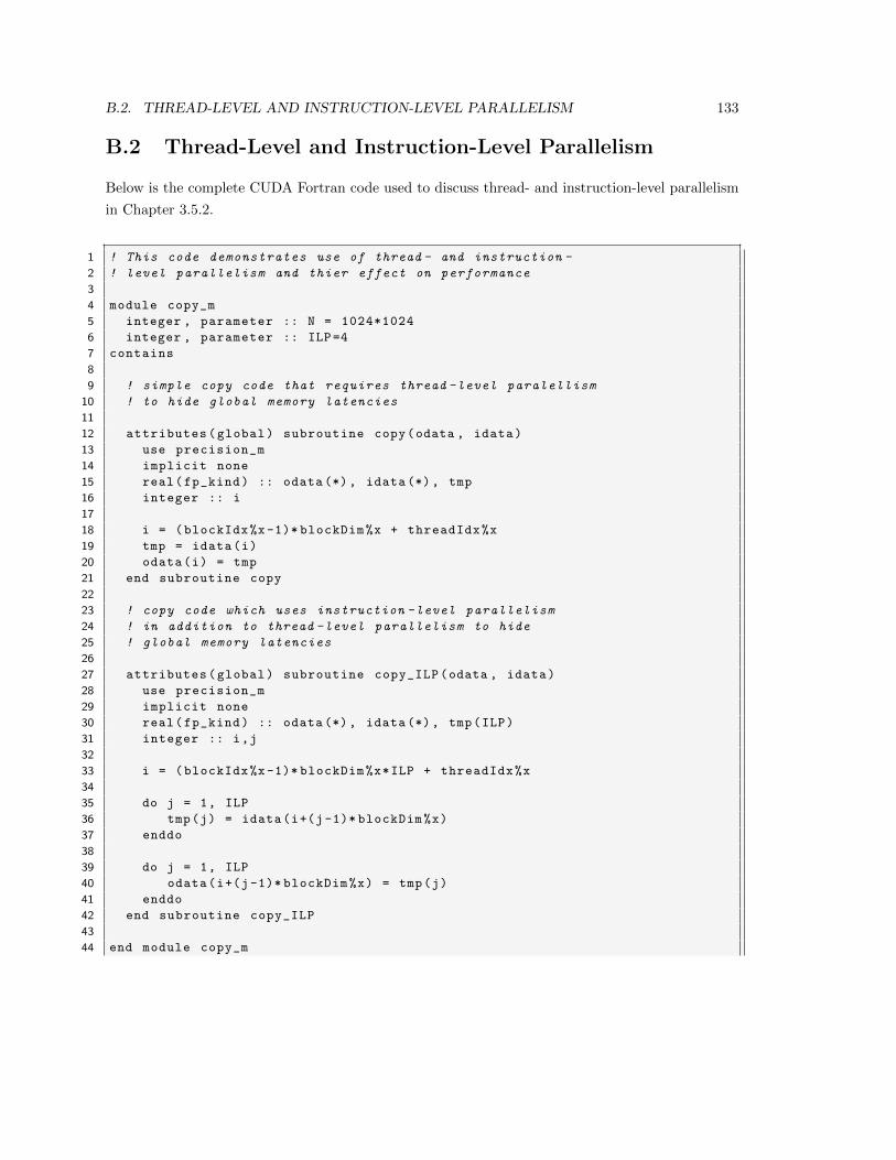
B.2. THREAD-LEVEL AND INSTRUCTION-LEVEL PARALLELISM 133
B.2 Thread-Level and Instruction-Level Parallelism
Below is the complete CUDA Fortran code used to discuss thread- and instruction-level parallelism
in Chapter 3.5.2.
1 ! This code demonstrates use of thread - and instruction -
2 ! level parallelism and thier effect on performance
3
4 module copy_m
5 integer , parameter :: N = 1024*1024
6 integer , parameter :: ILP=4
7 contains
8
9 ! simple copy code that requires thread -level paralellism
10 ! to hide global memory latencies
11
12 attributes(global) subroutine copy(odata , idata)
13 use precision_m
14 implicit none
15 real(fp_kind) :: odata (*), idata (*), tmp
16 integer :: i
17
18 i = (blockIdx%x-1)* blockDim%x + threadIdx%x
19 tmp = idata(i)
20 odata(i) = tmp
21 end subroutine copy
22
23 ! copy code which uses instruction -level parallelism
24 ! in addition to thread -level parallelism to hide
25 ! global memory latencies
26
27 attributes(global) subroutine copy_ILP(odata , idata)
28 use precision_m
29 implicit none
30 real(fp_kind) :: odata (*), idata (*), tmp(ILP)
31 integer :: i,j
32
33 i = (blockIdx%x-1)* blockDim%x*ILP + threadIdx%x
34
35 do j = 1, ILP
36 tmp(j) = idata(i+(j-1)* blockDim%x)
37 enddo
38
39 do j = 1, ILP
40 odata(i+(j-1)* blockDim%x) = tmp(j)
41 enddo
42 end subroutine copy_ILP
43
44 end module copy_m
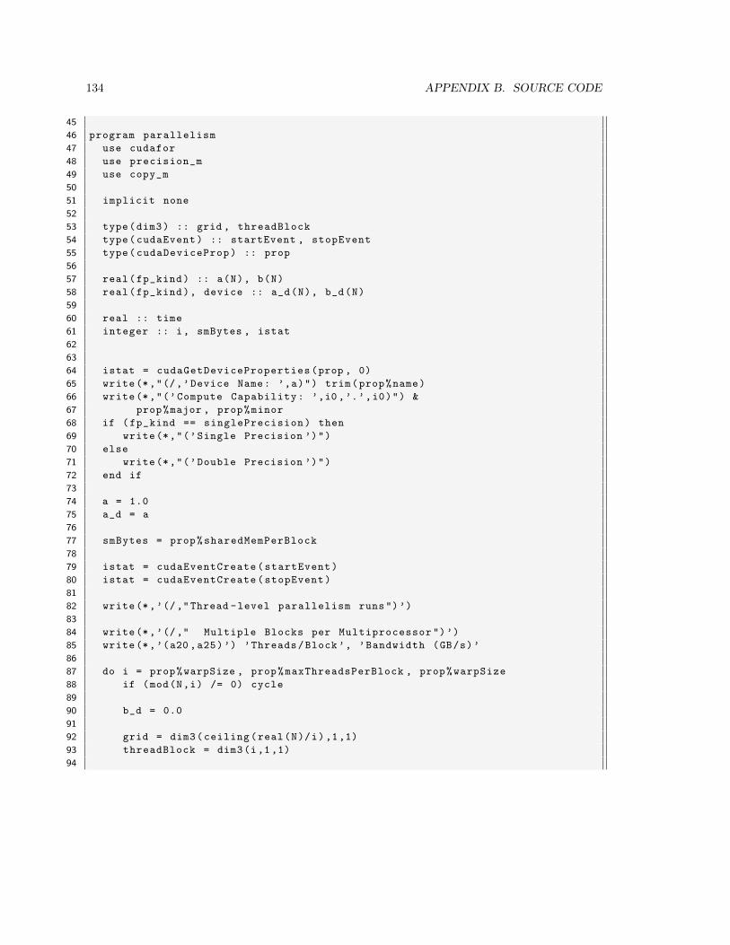
134 APPENDIX B. SOURCE CODE
45
46 program parallelism
47 use cudafor
48 use precision_m
49 use copy_m
50
51 implicit none
52
53 type(dim3) :: grid , threadBlock
54 type(cudaEvent) :: startEvent , stopEvent
55 type(cudaDeviceProp) :: prop
56
57 real(fp_kind) :: a(N), b(N)
58 real(fp_kind), device :: a_d(N), b_d(N)
59
60 real :: time
61 integer :: i, smBytes , istat
62
63
64 istat = cudaGetDeviceProperties(prop , 0)
65 write(*,"(/,’Device Name: ’,a)") trim(prop%name)
66 write(*,"(’Compute Capability: ’,i0 ,’.’,i0)") &
67 prop%major , prop%minor
68 if (fp_kind == singlePrecision) then
69 write(*,"(’Single Precision ’)")
70 else
71 write(*,"(’Double Precision ’)")
72 end if
73
74 a = 1.0
75 a_d = a
76
77 smBytes = prop%sharedMemPerBlock
78
79 istat = cudaEventCreate(startEvent)
80 istat = cudaEventCreate(stopEvent)
81
82 write(*,’(/,"Thread -level parallelism runs")’)
83
84 write(*,’(/," Multiple Blocks per Multiprocessor ")’)
85 write(*,’(a20 ,a25)’) ’Threads/Block’, ’Bandwidth (GB/s)’
86
87 do i = prop%warpSize , prop%maxThreadsPerBlock , prop%warpSize
88 if (mod(N,i) /= 0) cycle
89
90 b_d = 0.0
91
92 grid = dim3(ceiling(real(N)/i),1,1)
93 threadBlock = dim3(i,1,1)
94
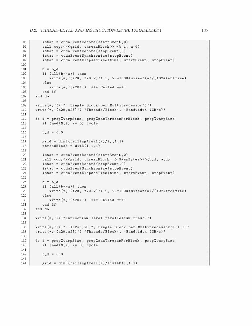
B.2. THREAD-LEVEL AND INSTRUCTION-LEVEL PARALLELISM 135
95 istat = cudaEventRecord(startEvent ,0)
96 call copy <<<grid , threadBlock >>>(b_d , a_d)
97 istat = cudaEventRecord(stopEvent ,0)
98 istat = cudaEventSynchronize(stopEvent)
99 istat = cudaEventElapsedTime(time , startEvent , stopEvent)
100
101 b = b_d
102 if (all(b==a)) then
103 write(*,’(i20 , f20.2)’) i, 2.*1000* sizeof(a)/(1024**3* time)
104 else
105 write(*,’(a20)’) ’*** Failed ***’
106 end if
107 end do
108
109 write(*,’(/," Single Block per Multiprocessor ")’)
110 write(*,’(a20 ,a25)’) ’Threads/Block’, ’Bandwidth (GB/s)’
111
112 do i = prop%warpSize , prop%maxThreadsPerBlock , prop%warpSize
113 if (mod(N,i) /= 0) cycle
114
115 b_d = 0.0
116
117 grid = dim3(ceiling(real(N)/i),1,1)
118 threadBlock = dim3(i,1,1)
119
120 istat = cudaEventRecord(startEvent ,0)
121 call copy <<<grid , threadBlock , 0.9* smBytes >>>(b_d , a_d)
122 istat = cudaEventRecord(stopEvent ,0)
123 istat = cudaEventSynchronize(stopEvent)
124 istat = cudaEventElapsedTime(time , startEvent , stopEvent)
125
126 b = b_d
127 if (all(b==a)) then
128 write(*,’(i20 , f20.2)’) i, 2.*1000* sizeof(a)/(1024**3* time)
129 else
130 write(*,’(a20)’) ’*** Failed ***’
131 end if
132 end do
133
134 write(*,’(/," Intruction -level parallelism runs")’)
135
136 write(*,’(/," ILP=",i0 ,", Single Block per Multiprocessor ")’) ILP
137 write(*,’(a20 ,a25)’) ’Threads/Block’, ’Bandwidth (GB/s)’
138
139 do i = prop%warpSize , prop%maxThreadsPerBlock , prop%warpSize
140 if (mod(N,i) /= 0) cycle
141
142 b_d = 0.0
143
144 grid = dim3(ceiling(real(N)/(i*ILP)),1,1)
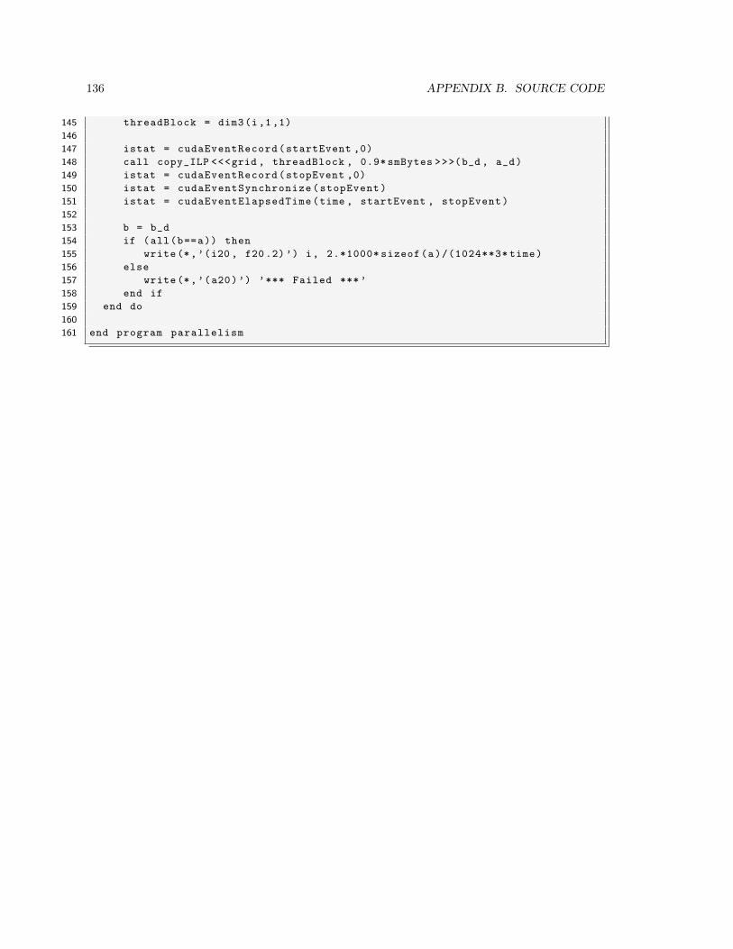
136 APPENDIX B. SOURCE CODE
145 threadBlock = dim3(i,1,1)
146
147 istat = cudaEventRecord(startEvent ,0)
148 call copy_ILP <<<grid , threadBlock , 0.9* smBytes >>>(b_d , a_d)
149 istat = cudaEventRecord(stopEvent ,0)
150 istat = cudaEventSynchronize(stopEvent)
151 istat = cudaEventElapsedTime(time , startEvent , stopEvent)
152
153 b = b_d
154 if (all(b==a)) then
155 write(*,’(i20 , f20.2)’) i, 2.*1000* sizeof(a)/(1024**3* time)
156 else
157 write(*,’(a20)’) ’*** Failed ***’
158 end if
159 end do
160
161 end program parallelism

B.3. FINITE DIFFERENCE CODE 137
B.3 Finite Difference Code
Below is the complete CUDA Fortran code used in the Finite Difference case study of Chapter 5.
The derivative module containing the kernels is:
1 ! This file contains the setup host code and kernels for
2 ! calculating derivatives using a 9-point finite difference
3 ! stencil
4
5 module derivative_m
6 use cudafor
7 use precision_m
8
9 integer , parameter :: mx = 64, my = 64, mz = 64
10 real(fp_kind) :: x(mx), y(my), z(mz)
11
12 ! shared memory tiles will be m*-by -* Pencils
13 ! sPencils is used when each thread calculates
14 ! the derivative at one point
15 ! lPencils is used for coalescing in y and z
16 ! where each thread has to calculate the
17 ! derivative at mutiple points
18
19 integer , parameter :: sPencils = 4 ! small # pencils
20 integer , parameter :: lPencils = 32 ! large # pencils
21
22 type(dim3) :: grid_sp (3), block_sp (3)
23 type(dim3) :: grid_lp (3), block_lp (3)
24
25 ! stencil coefficients
26
27 real(fp_kind), constant :: ax_c , bx_c , cx_c , dx_c
28 real(fp_kind), constant :: ay_c , by_c , cy_c , dy_c
29 real(fp_kind), constant :: az_c , bz_c , cz_c , dz_c
30
31 contains
32
33 ! host routine to set constant data
34
35 subroutine setDerivativeParameters ()
36
37 implicit none
38
39 real(fp_kind) :: dsinv
40 integer :: i, j, k
41
42 ! check to make sure dimensions are integral multiples of sPencils
43 if (mod(my ,sPencils) /= 0) then
44 write (*,*) ’"my" must be an integral multiple of sPencils ’
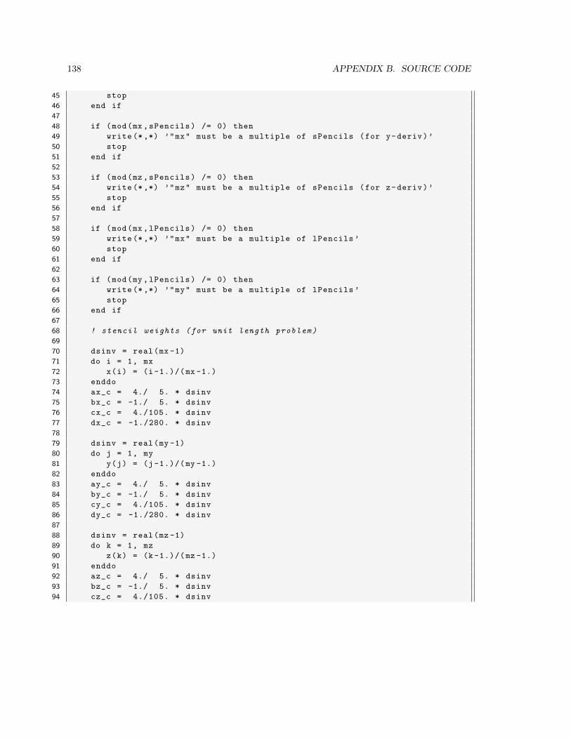
138 APPENDIX B. SOURCE CODE
45 stop
46 end if
47
48 if (mod(mx ,sPencils) /= 0) then
49 write (*,*) ’"mx" must be a multiple of sPencils (for y-deriv)’
50 stop
51 end if
52
53 if (mod(mz ,sPencils) /= 0) then
54 write (*,*) ’"mz" must be a multiple of sPencils (for z-deriv)’
55 stop
56 end if
57
58 if (mod(mx ,lPencils) /= 0) then
59 write (*,*) ’"mx" must be a multiple of lPencils ’
60 stop
61 end if
62
63 if (mod(my ,lPencils) /= 0) then
64 write (*,*) ’"my" must be a multiple of lPencils ’
65 stop
66 end if
67
68 ! stencil weights (for unit length problem)
69
70 dsinv = real(mx -1)
71 do i = 1, mx
72 x(i) = (i -1.)/(mx -1.)
73 enddo
74 ax_c = 4./ 5. * dsinv
75 bx_c = -1./ 5. * dsinv
76 cx_c = 4./105. * dsinv
77 dx_c = -1./280. * dsinv
78
79 dsinv = real(my -1)
80 do j = 1, my
81 y(j) = (j -1.)/(my -1.)
82 enddo
83 ay_c = 4./ 5. * dsinv
84 by_c = -1./ 5. * dsinv
85 cy_c = 4./105. * dsinv
86 dy_c = -1./280. * dsinv
87
88 dsinv = real(mz -1)
89 do k = 1, mz
90 z(k) = (k -1.)/(mz -1.)
91 enddo
92 az_c = 4./ 5. * dsinv
93 bz_c = -1./ 5. * dsinv
94 cz_c = 4./105. * dsinv
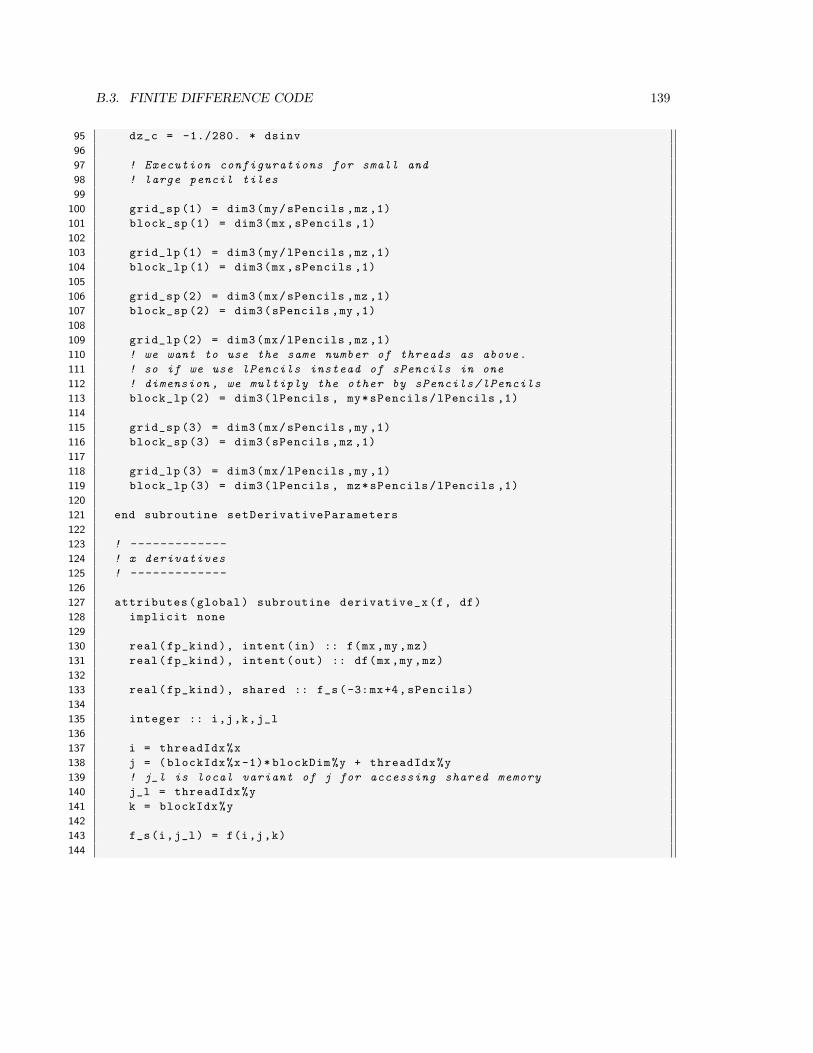
B.3. FINITE DIFFERENCE CODE 139
95 dz_c = -1./280. * dsinv
96
97 ! Execution configurations for small and
98 ! large pencil tiles
99
100 grid_sp (1) = dim3(my/sPencils ,mz ,1)
101 block_sp (1) = dim3(mx,sPencils ,1)
102
103 grid_lp (1) = dim3(my/lPencils ,mz ,1)
104 block_lp (1) = dim3(mx,sPencils ,1)
105
106 grid_sp (2) = dim3(mx/sPencils ,mz ,1)
107 block_sp (2) = dim3(sPencils ,my ,1)
108
109 grid_lp (2) = dim3(mx/lPencils ,mz ,1)
110 ! we want to use the same number of threads as above.
111 ! so if we use lPencils instead of sPencils in one
112 ! dimension , we multiply the other by sPencils/lPencils
113 block_lp (2) = dim3(lPencils , my*sPencils/lPencils ,1)
114
115 grid_sp (3) = dim3(mx/sPencils ,my ,1)
116 block_sp (3) = dim3(sPencils ,mz ,1)
117
118 grid_lp (3) = dim3(mx/lPencils ,my ,1)
119 block_lp (3) = dim3(lPencils , mz*sPencils/lPencils ,1)
120
121 end subroutine setDerivativeParameters
122
123 ! -------------
124 ! x derivatives
125 ! -------------
126
127 attributes(global) subroutine derivative_x(f, df)
128 implicit none
129
130 real(fp_kind), intent(in) :: f(mx,my,mz)
131 real(fp_kind), intent(out) :: df(mx,my,mz)
132
133 real(fp_kind), shared :: f_s(-3:mx+4,sPencils)
134
135 integer :: i,j,k,j_l
136
137 i = threadIdx%x
138 j = (blockIdx%x-1)* blockDim%y + threadIdx%y
139 ! j_l is local variant of j for accessing shared memory
140 j_l = threadIdx%y
141 k = blockIdx%y
142
143 f_s(i,j_l) = f(i,j,k)
144
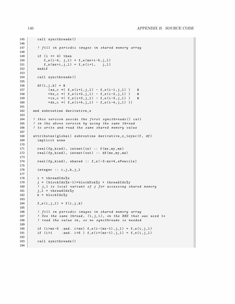
140 APPENDIX B. SOURCE CODE
145 call syncthreads ()
146
147 ! fill in periodic images in shared memory array
148
149 if (i <= 4) then
150 f_s(i-4, j_l) = f_s(mx+i-5,j_l)
151 f_s(mx+i,j_l) = f_s(i+1, j_l)
152 endif
153
154 call syncthreads ()
155
156 df(i,j,k) = &
157 (ax_c *( f_s(i+1,j_l) - f_s(i-1,j_l) ) &
158 +bx_c *( f_s(i+2,j_l) - f_s(i-2,j_l) ) &
159 +cx_c *( f_s(i+3,j_l) - f_s(i-3,j_l) ) &
160 +dx_c *( f_s(i+4,j_l) - f_s(i-4,j_l) ))
161
162 end subroutine derivative_x
163
164 ! this version avoids the first syncthreads () call
165 ! in the above version by using the same thread
166 ! to write and read the same shared memory value
167
168 attributes(global) subroutine derivative_x_1sync(f, df)
169 implicit none
170
171 real(fp_kind), intent(in) :: f(mx,my,mz)
172 real(fp_kind), intent(out) :: df(mx,my,mz)
173
174 real(fp_kind), shared :: f_s(-3:mx+4,sPencils)
175
176 integer :: i,j,k,j_l
177
178 i = threadIdx%x
179 j = (blockIdx%x-1)* blockDim%y + threadIdx%y
180 ! j_l is local variant of j for accessing shared memory
181 j_l = threadIdx%y
182 k = blockIdx%y
183
184 f_s(i,j_l) = f(i,j,k)
185
186 ! fill in periodic images in shared memory array
187 ! Use the same thread , (i,j_l), on the RHS that was used to
188 ! read the value in , so no syncthreads is needed
189
190 if (i>mx -5 .and. i<mx) f_s(i-(mx -1),j_l) = f_s(i,j_l)
191 if (i>1 .and. i<6 ) f_s(i+(mx -1),j_l) = f_s(i,j_l)
192
193 call syncthreads ()
194
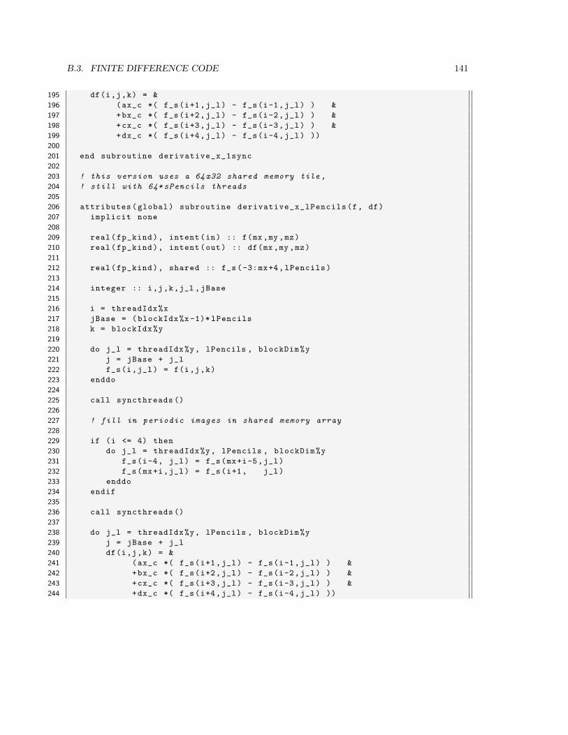
B.3. FINITE DIFFERENCE CODE 141
195 df(i,j,k) = &
196 (ax_c *( f_s(i+1,j_l) - f_s(i-1,j_l) ) &
197 +bx_c *( f_s(i+2,j_l) - f_s(i-2,j_l) ) &
198 +cx_c *( f_s(i+3,j_l) - f_s(i-3,j_l) ) &
199 +dx_c *( f_s(i+4,j_l) - f_s(i-4,j_l) ))
200
201 end subroutine derivative_x_1sync
202
203 ! this version uses a 64x32 shared memory tile ,
204 ! still with 64* sPencils threads
205
206 attributes(global) subroutine derivative_x_lPencils(f, df)
207 implicit none
208
209 real(fp_kind), intent(in) :: f(mx,my,mz)
210 real(fp_kind), intent(out) :: df(mx,my,mz)
211
212 real(fp_kind), shared :: f_s(-3:mx+4,lPencils)
213
214 integer :: i,j,k,j_l ,jBase
215
216 i = threadIdx%x
217 jBase = (blockIdx%x-1)* lPencils
218 k = blockIdx%y
219
220 do j_l = threadIdx%y, lPencils , blockDim%y
221 j = jBase + j_l
222 f_s(i,j_l) = f(i,j,k)
223 enddo
224
225 call syncthreads ()
226
227 ! fill in periodic images in shared memory array
228
229 if (i <= 4) then
230 do j_l = threadIdx%y, lPencils , blockDim%y
231 f_s(i-4, j_l) = f_s(mx+i-5,j_l)
232 f_s(mx+i,j_l) = f_s(i+1, j_l)
233 enddo
234 endif
235
236 call syncthreads ()
237
238 do j_l = threadIdx%y, lPencils , blockDim%y
239 j = jBase + j_l
240 df(i,j,k) = &
241 (ax_c *( f_s(i+1,j_l) - f_s(i-1,j_l) ) &
242 +bx_c *( f_s(i+2,j_l) - f_s(i-2,j_l) ) &
243 +cx_c *( f_s(i+3,j_l) - f_s(i-3,j_l) ) &
244 +dx_c *( f_s(i+4,j_l) - f_s(i-4,j_l) ))
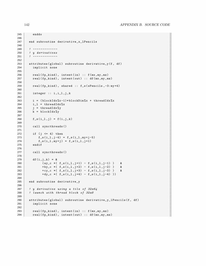
142 APPENDIX B. SOURCE CODE
245 enddo
246
247 end subroutine derivative_x_lPencils
248
249 ! -------------
250 ! y derivatives
251 ! -------------
252
253 attributes(global) subroutine derivative_y(f, df)
254 implicit none
255
256 real(fp_kind), intent(in) :: f(mx,my,mz)
257 real(fp_kind), intent(out) :: df(mx,my,mz)
258
259 real(fp_kind), shared :: f_s(sPencils ,-3:my+4)
260
261 integer :: i,i_l ,j,k
262
263 i = (blockIdx%x-1)* blockDim%x + threadIdx%x
264 i_l = threadIdx%x
265 j = threadIdx%y
266 k = blockIdx%y
267
268 f_s(i_l ,j) = f(i,j,k)
269
270 call syncthreads ()
271
272 if (j <= 4) then
273 f_s(i_l ,j-4) = f_s(i_l ,my+j-5)
274 f_s(i_l ,my+j) = f_s(i_l ,j+1)
275 endif
276
277 call syncthreads ()
278
279 df(i,j,k) = &
280 (ay_c *( f_s(i_l ,j+1) - f_s(i_l ,j-1) ) &
281 +by_c *( f_s(i_l ,j+2) - f_s(i_l ,j-2) ) &
282 +cy_c *( f_s(i_l ,j+3) - f_s(i_l ,j-3) ) &
283 +dy_c *( f_s(i_l ,j+4) - f_s(i_l ,j-4) ))
284
285 end subroutine derivative_y
286
287 ! y derivative using a tile of 32x64
288 ! launch with thread block of 32x8
289
290 attributes(global) subroutine derivative_y_lPencils(f, df)
291 implicit none
292
293 real(fp_kind), intent(in) :: f(mx,my,mz)
294 real(fp_kind), intent(out) :: df(mx,my,mz)
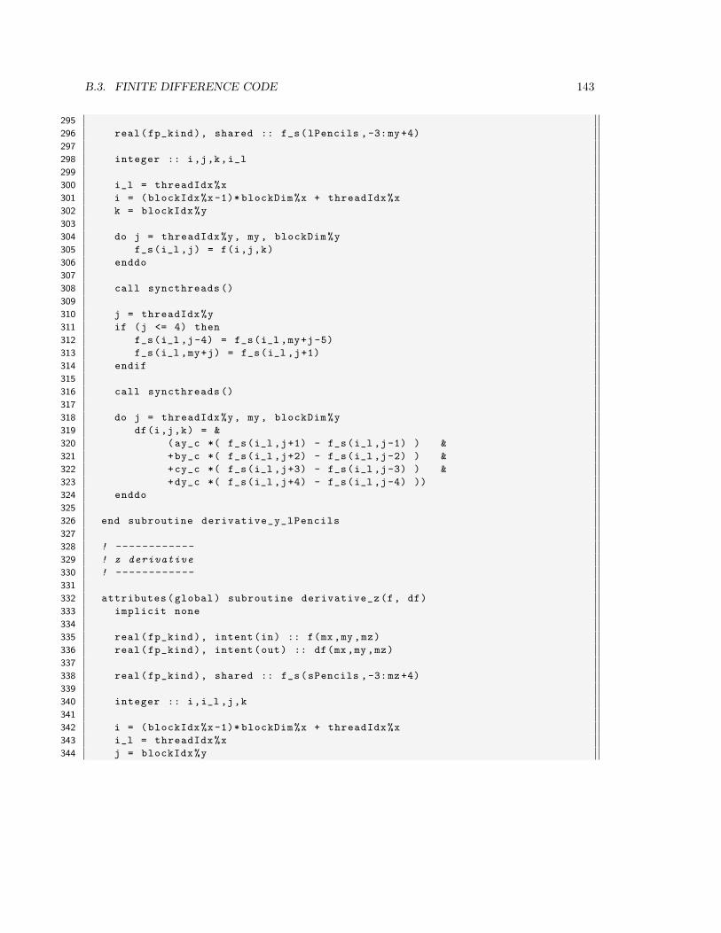
B.3. FINITE DIFFERENCE CODE 143
295
296 real(fp_kind), shared :: f_s(lPencils ,-3:my+4)
297
298 integer :: i,j,k,i_l
299
300 i_l = threadIdx%x
301 i = (blockIdx%x-1)* blockDim%x + threadIdx%x
302 k = blockIdx%y
303
304 do j = threadIdx%y, my, blockDim%y
305 f_s(i_l ,j) = f(i,j,k)
306 enddo
307
308 call syncthreads ()
309
310 j = threadIdx%y
311 if (j <= 4) then
312 f_s(i_l ,j-4) = f_s(i_l ,my+j-5)
313 f_s(i_l ,my+j) = f_s(i_l ,j+1)
314 endif
315
316 call syncthreads ()
317
318 do j = threadIdx%y, my, blockDim%y
319 df(i,j,k) = &
320 (ay_c *( f_s(i_l ,j+1) - f_s(i_l ,j-1) ) &
321 +by_c *( f_s(i_l ,j+2) - f_s(i_l ,j-2) ) &
322 +cy_c *( f_s(i_l ,j+3) - f_s(i_l ,j-3) ) &
323 +dy_c *( f_s(i_l ,j+4) - f_s(i_l ,j-4) ))
324 enddo
325
326 end subroutine derivative_y_lPencils
327
328 ! ------------
329 ! z derivative
330 ! ------------
331
332 attributes(global) subroutine derivative_z(f, df)
333 implicit none
334
335 real(fp_kind), intent(in) :: f(mx,my,mz)
336 real(fp_kind), intent(out) :: df(mx,my,mz)
337
338 real(fp_kind), shared :: f_s(sPencils ,-3:mz+4)
339
340 integer :: i,i_l ,j,k
341
342 i = (blockIdx%x-1)* blockDim%x + threadIdx%x
343 i_l = threadIdx%x
344 j = blockIdx%y

144 APPENDIX B. SOURCE CODE
345 k = threadIdx%y
346
347 f_s(i_l ,k) = f(i,j,k)
348
349 call syncthreads ()
350
351 if (k <= 4) then
352 f_s(i_l ,k-4) = f_s(i_l ,mz+k-5)
353 f_s(i_l ,mz+k) = f_s(i_l ,k+1)
354 endif
355
356 call syncthreads ()
357
358 df(i,j,k) = &
359 (az_c *( f_s(i_l ,k+1) - f_s(i_l ,k-1) ) &
360 +bz_c *( f_s(i_l ,k+2) - f_s(i_l ,k-2) ) &
361 +cz_c *( f_s(i_l ,k+3) - f_s(i_l ,k-3) ) &
362 +dz_c *( f_s(i_l ,k+4) - f_s(i_l ,k-4) ))
363
364 end subroutine derivative_z
365
366
367 attributes(global) subroutine derivative_z_lPencils(f, df)
368 implicit none
369
370 real(fp_kind), intent(in) :: f(mx,my,mz)
371 real(fp_kind), intent(out) :: df(mx,my,mz)
372
373 real(fp_kind), shared :: f_s(lPencils ,-3:mz+4)
374
375 integer :: i,i_l ,j,k
376
377 i = (blockIdx%x-1)* blockDim%x + threadIdx%x
378 i_l = threadIdx%x
379 j = blockIdx%y
380
381 do k = threadIdx%y, mz, blockDim%y
382 f_s(i_l ,k) = f(i,j,k)
383 enddo
384
385 call syncthreads ()
386
387 k = threadIdx%y
388 if (k <= 4) then
389 f_s(i_l ,k-4) = f_s(i_l ,mz+k-5)
390 f_s(i_l ,mz+k) = f_s(i_l ,k+1)
391 endif
392
393 call syncthreads ()
394
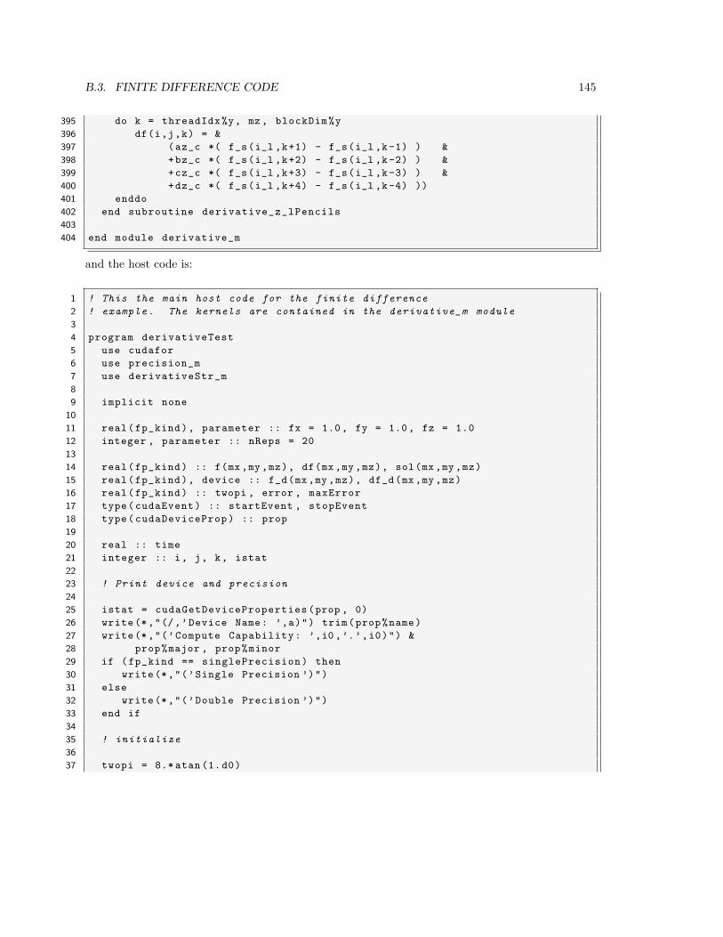
B.3. FINITE DIFFERENCE CODE 145
395 do k = threadIdx%y, mz, blockDim%y
396 df(i,j,k) = &
397 (az_c *( f_s(i_l ,k+1) - f_s(i_l ,k-1) ) &
398 +bz_c *( f_s(i_l ,k+2) - f_s(i_l ,k-2) ) &
399 +cz_c *( f_s(i_l ,k+3) - f_s(i_l ,k-3) ) &
400 +dz_c *( f_s(i_l ,k+4) - f_s(i_l ,k-4) ))
401 enddo
402 end subroutine derivative_z_lPencils
403
404 end module derivative_m
and the host code is:
1 ! This the main host code for the finite difference
2 ! example. The kernels are contained in the derivative_m module
3
4 program derivativeTest
5 use cudafor
6 use precision_m
7 use derivativeStr_m
8
9 implicit none
10
11 real(fp_kind), parameter :: fx = 1.0, fy = 1.0, fz = 1.0
12 integer , parameter :: nReps = 20
13
14 real(fp_kind) :: f(mx,my,mz), df(mx,my,mz), sol(mx,my,mz)
15 real(fp_kind), device :: f_d(mx,my,mz), df_d(mx,my,mz)
16 real(fp_kind) :: twopi , error , maxError
17 type(cudaEvent) :: startEvent , stopEvent
18 type(cudaDeviceProp) :: prop
19
20 real :: time
21 integer :: i, j, k, istat
22
23 ! Print device and precision
24
25 istat = cudaGetDeviceProperties(prop , 0)
26 write(*,"(/,’Device Name: ’,a)") trim(prop%name)
27 write(*,"(’Compute Capability: ’,i0 ,’.’,i0)") &
28 prop%major , prop%minor
29 if (fp_kind == singlePrecision) then
30 write(*,"(’Single Precision ’)")
31 else
32 write(*,"(’Double Precision ’)")
33 end if
34
35 ! initialize
36
37 twopi = 8.* atan (1.d0)
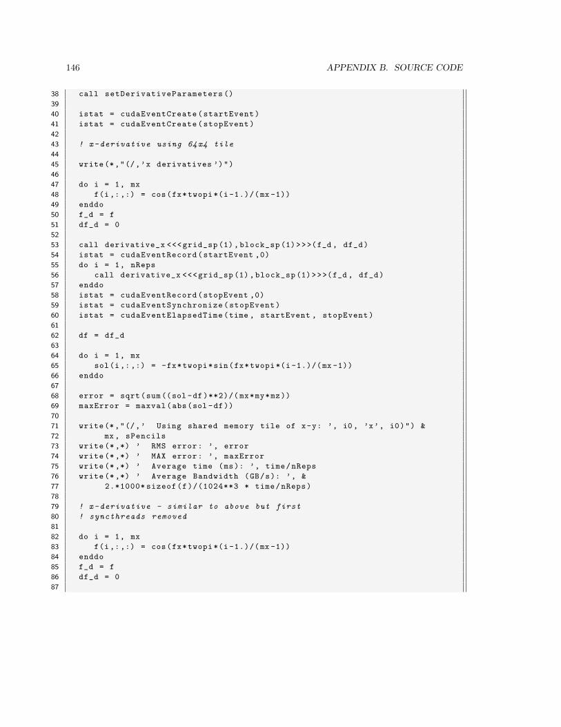
146 APPENDIX B. SOURCE CODE
38 call setDerivativeParameters ()
39
40 istat = cudaEventCreate(startEvent)
41 istat = cudaEventCreate(stopEvent)
42
43 ! x-derivative using 64x4 tile
44
45 write(*,"(/,’x derivatives ’)")
46
47 do i = 1, mx
48 f(i,:,:) = cos(fx*twopi*(i -1.)/(mx -1))
49 enddo
50 f_d = f
51 df_d = 0
52
53 call derivative_x <<<grid_sp (1), block_sp (1)>>>(f_d , df_d)
54 istat = cudaEventRecord(startEvent ,0)
55 do i = 1, nReps
56 call derivative_x <<<grid_sp (1), block_sp (1)>>>(f_d , df_d)
57 enddo
58 istat = cudaEventRecord(stopEvent ,0)
59 istat = cudaEventSynchronize(stopEvent)
60 istat = cudaEventElapsedTime(time , startEvent , stopEvent)
61
62 df = df_d
63
64 do i = 1, mx
65 sol(i,:,:) = -fx*twopi*sin(fx*twopi*(i -1.)/(mx -1))
66 enddo
67
68 error = sqrt(sum((sol -df )**2)/( mx*my*mz))
69 maxError = maxval(abs(sol -df))
70
71 write(*,"(/,’ Using shared memory tile of x-y: ’, i0 , ’x’, i0)") &
72 mx , sPencils
73 write (*,*) ’ RMS error: ’, error
74 write (*,*) ’ MAX error: ’, maxError
75 write (*,*) ’ Average time (ms): ’, time/nReps
76 write (*,*) ’ Average Bandwidth (GB/s): ’, &
77 2.*1000* sizeof(f)/(1024**3 * time/nReps)
78
79 ! x-derivative - similar to above but first
80 ! syncthreads removed
81
82 do i = 1, mx
83 f(i,:,:) = cos(fx*twopi*(i -1.)/(mx -1))
84 enddo
85 f_d = f
86 df_d = 0
87
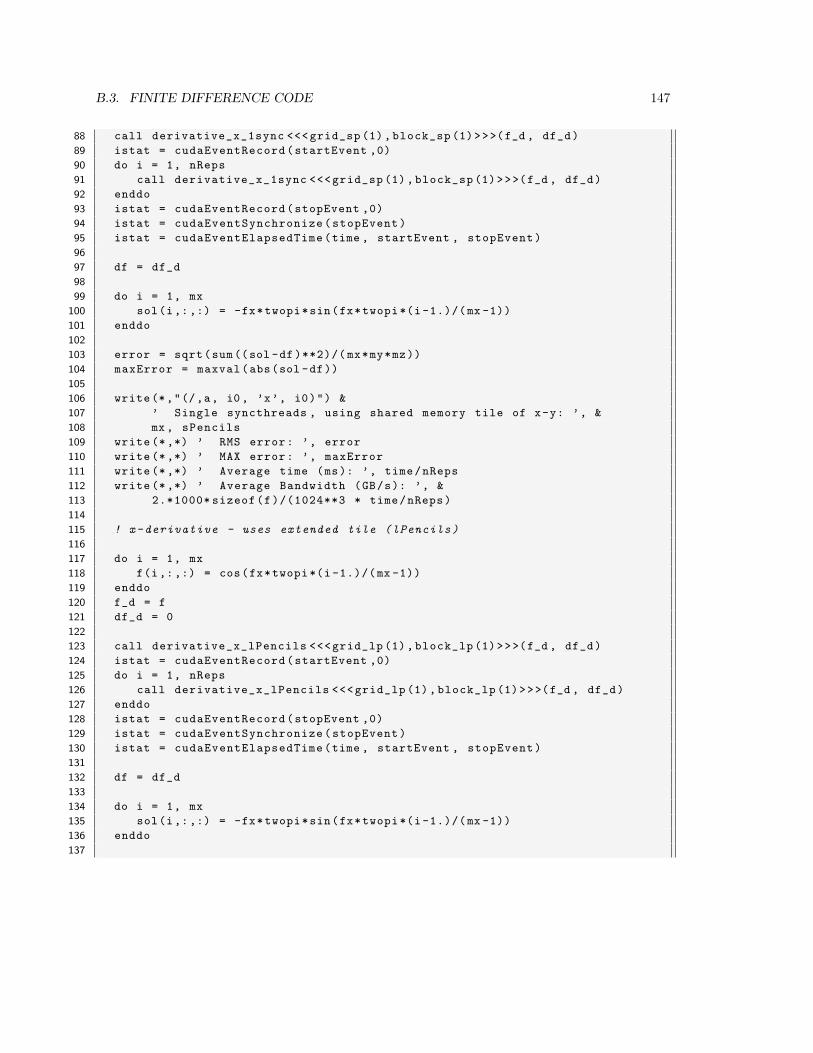
B.3. FINITE DIFFERENCE CODE 147
88 call derivative_x_1sync <<<grid_sp (1), block_sp (1)>>>(f_d , df_d)
89 istat = cudaEventRecord(startEvent ,0)
90 do i = 1, nReps
91 call derivative_x_1sync <<<grid_sp (1), block_sp (1)>>>(f_d , df_d)
92 enddo
93 istat = cudaEventRecord(stopEvent ,0)
94 istat = cudaEventSynchronize(stopEvent)
95 istat = cudaEventElapsedTime(time , startEvent , stopEvent)
96
97 df = df_d
98
99 do i = 1, mx
100 sol(i,:,:) = -fx*twopi*sin(fx*twopi*(i -1.)/(mx -1))
101 enddo
102
103 error = sqrt(sum((sol -df )**2)/( mx*my*mz))
104 maxError = maxval(abs(sol -df))
105
106 write(*,"(/,a, i0 , ’x’, i0)") &
107 ’ Single syncthreads , using shared memory tile of x-y: ’, &
108 mx , sPencils
109 write (*,*) ’ RMS error: ’, error
110 write (*,*) ’ MAX error: ’, maxError
111 write (*,*) ’ Average time (ms): ’, time/nReps
112 write (*,*) ’ Average Bandwidth (GB/s): ’, &
113 2.*1000* sizeof(f)/(1024**3 * time/nReps)
114
115 ! x-derivative - uses extended tile (lPencils)
116
117 do i = 1, mx
118 f(i,:,:) = cos(fx*twopi*(i -1.)/(mx -1))
119 enddo
120 f_d = f
121 df_d = 0
122
123 call derivative_x_lPencils <<<grid_lp (1), block_lp (1)>>>(f_d , df_d)
124 istat = cudaEventRecord(startEvent ,0)
125 do i = 1, nReps
126 call derivative_x_lPencils <<<grid_lp (1), block_lp (1)>>>(f_d , df_d)
127 enddo
128 istat = cudaEventRecord(stopEvent ,0)
129 istat = cudaEventSynchronize(stopEvent)
130 istat = cudaEventElapsedTime(time , startEvent , stopEvent)
131
132 df = df_d
133
134 do i = 1, mx
135 sol(i,:,:) = -fx*twopi*sin(fx*twopi*(i -1.)/(mx -1))
136 enddo
137
148 APPENDIX B. SOURCE CODE
138 error = sqrt(sum((sol -df )**2)/( mx*my*mz))
139 maxError = maxval(abs(sol -df))
140
141 write(*,"(/,’ Using shared memory tile of x-y: ’, i0 , ’x’, i0)") &
142 mx , lPencils
143 write (*,*) ’ RMS error: ’, error
144 write (*,*) ’ MAX error: ’, maxError
145 write (*,*) ’ Average time (ms): ’, time/nReps
146 write (*,*) ’ Average Bandwidth (GB/s): ’, &
147 2.*1000* sizeof(f)/(1024**3 * time/nReps)
148
149 ! y-derivative
150
151 write(*,"(/,’y derivatives ’)")
152
153 do j = 1, my
154 f(:,j,:) = cos(fy*twopi*(j -1.)/(my -1))
155 enddo
156 f_d = f
157 df_d = 0
158
159 call derivative_y <<<grid_sp (2), block_sp (2)>>>(f_d , df_d)
160 istat = cudaEventRecord(startEvent ,0)
161 do i = 1, nReps
162 call derivative_y <<<grid_sp (2), block_sp (2)>>>(f_d , df_d)
163 enddo
164 istat = cudaEventRecord(stopEvent ,0)
165 istat = cudaEventSynchronize(stopEvent)
166 istat = cudaEventElapsedTime(time , startEvent , stopEvent)
167
168 df = df_d
169
170 do j = 1, my
171 sol(:,j,:) = -fy*twopi*sin(fy*twopi*(j -1.)/(my -1))
172 enddo
173
174 error = sqrt(sum((sol -df )**2)/( mx*my*mz))
175 maxError = maxval(abs(sol -df))
176
177 write(*,"(/,’ Using shared memory tile of x-y: ’, i0 , ’x’, i0)") &
178 sPencils , my
179 write (*,*) ’ RMS error: ’, error
180 write (*,*) ’ MAX error: ’, maxError
181 write (*,*) ’ Average time (ms): ’, time/nReps
182 write (*,*) ’ Average Bandwidth (GB/s): ’, &
183 2.*1000* sizeof(f)/(1024**3 * time/nReps)
184
185 ! y-derivative lPencils
186
187 do j = 1, my

B.3. FINITE DIFFERENCE CODE 149
188 f(:,j,:) = cos(fy*twopi*(j -1.)/(my -1))
189 enddo
190 f_d = f
191 df_d = 0
192
193 call derivative_y_lPencils <<<grid_lp (2), block_lp (2)>>>(f_d , df_d)
194 istat = cudaEventRecord(startEvent ,0)
195 do i = 1, nReps
196 call derivative_y_lPencils <<<grid_lp (2), block_lp (2)>>>(f_d , df_d)
197 enddo
198 istat = cudaEventRecord(stopEvent ,0)
199 istat = cudaEventSynchronize(stopEvent)
200 istat = cudaEventElapsedTime(time , startEvent , stopEvent)
201
202 df = df_d
203
204 do j = 1, my
205 sol(:,j,:) = -fy*twopi*sin(fy*twopi*(j -1.)/(my -1))
206 enddo
207
208 error = sqrt(sum((sol -df )**2)/( mx*my*mz))
209 maxError = maxval(abs(sol -df))
210
211 write(*,"(/,’ Using shared memory tile of x-y: ’, i0 , ’x’, i0)") &
212 lPencils , my
213 write (*,*) ’ RMS error: ’, error
214 write (*,*) ’ MAX error: ’, maxError
215 write (*,*) ’ Average time (ms): ’, time/nReps
216 write (*,*) ’ Average Bandwidth (GB/s): ’, &
217 2.*1000* sizeof(f)/(1024**3 * time/nReps)
218
219 ! z-derivative
220
221 write(*,"(/,’z derivatives ’)")
222
223 do k = 1, mz
224 f(:,:,k) = cos(fz*twopi*(k -1.)/(mz -1))
225 enddo
226 f_d = f
227 df_d = 0
228
229 call derivative_z <<<grid_sp (3), block_sp (3)>>>(f_d , df_d)
230 istat = cudaEventRecord(startEvent ,0)
231 do i = 1, nReps
232 call derivative_z <<<grid_sp (3), block_sp (3)>>>(f_d , df_d)
233 enddo
234 istat = cudaEventRecord(stopEvent ,0)
235 istat = cudaEventSynchronize(stopEvent)
236 istat = cudaEventElapsedTime(time , startEvent , stopEvent)
237

150 APPENDIX B. SOURCE CODE
238 df = df_d
239
240 do k = 1, mz
241 sol(:,:,k) = -fz*twopi*sin(fz*twopi*(k -1.)/(mz -1))
242 enddo
243
244 error = sqrt(sum((sol -df )**2)/( mx*my*mz))
245 maxError = maxval(abs(sol -df))
246
247 write(*,"(/,’ Using shared memory tile of x-z: ’, i0 , ’x’, i0)") &
248 sPencils , mz
249 write (*,*) ’ RMS error: ’, error
250 write (*,*) ’ MAX error: ’, maxError
251 write (*,*) ’ Average time (ms): ’, time/nReps
252 write (*,*) ’ Average Bandwidth (GB/s): ’, &
253 2.*1000* sizeof(f)/(1024**3 * time/nReps)
254
255 ! z-derivative lPencils
256
257 do k = 1, mz
258 f(:,:,k) = cos(fz*twopi*(k -1.)/(mz -1))
259 enddo
260 f_d = f
261 df_d = 0
262
263 call derivative_z_lPencils <<<grid_lp (3), block_lp (3)>>>(f_d , df_d)
264 istat = cudaEventRecord(startEvent ,0)
265 do i = 1, nReps
266 call derivative_z_lPencils <<<grid_lp (3), block_lp (3)>>>(f_d , df_d)
267 enddo
268 istat = cudaEventRecord(stopEvent ,0)
269 istat = cudaEventSynchronize(stopEvent)
270 istat = cudaEventElapsedTime(time , startEvent , stopEvent)
271
272 df = df_d
273
274 do k = 1, mz
275 sol(:,:,k) = -fz*twopi*sin(fz*twopi*(k -1.)/(mz -1))
276 enddo
277
278 error = sqrt(sum((sol -df )**2)/( mx*my*mz))
279 maxError = maxval(abs(sol -df))
280
281 write(*,"(/,’ Using shared memory tile of x-z: ’, i0 , ’x’, i0)") &
282 lPencils , mz
283 write (*,*) ’ RMS error: ’, error
284 write (*,*) ’ MAX error: ’, maxError
285 write (*,*) ’ Average time (ms): ’, time/nReps
286 write (*,*) ’ Average Bandwidth (GB/s): ’, &
287 2.*1000* sizeof(f)/(1024**3 * time/nReps)

B.3. FINITE DIFFERENCE CODE 151
288 write (*,*)
289
290 end program derivativeTest

152 APPENDIX B. SOURCE CODE