Embed Size (px)
Citation preview

Currency Risk and International Diversification of Property Investments: A
Singaporean Investor’s Viewpoint
Kwame Addae-Dapaah
National University of Singapore
And
Yeo Hui Siang, Trecia Investment Executive, Far East Organization, Singapore
JEL Classification Code: C12, G11 Key Words: Currency risk, international diversification, property investment, return, risk, Singapore
Please send correspondence to:
Dr Kwame Addae-Dapaah, Department of Real Estate, SDE, National University of Singapore,
4 Architecture Drive, Singapore 117566
Tel: (65) 874 3417 Fax: (65) 775 5502
E-mail: [email protected]
Eighth European Real Estate Society Conference, Alicante June 26-29, 2001
Please do not quote without authors’ written approval
2
Abstract
International diversification of investments has been acclaimed to provide enhanced portfolio return
and reduced risk. However exchange rate volatility could negate the enhanced return. Therefore, this
paper is aimed at evaluating the impact of currency risk on the return/risk of international direct
property investments. The paper is based on the return data for fourteen countries from 1986 to 1997
inclusive. Because of the peculiar nature of real property investment, which precludes short selling
and riskless borrowing, Matlab Optimization toolbox (a computer software) the optimal portfolio
composition from which the efficient frontiers are plotted. Furthermore, the Singapore dollar is used
as the base currency to reflect the viewpoint of Singapore investors although analyses based on the
currency of any of the sampled countries should produce similar results. Analyses of the return data
reveal that currency risk had a devastating effect on the investment return for some individual
countries albeit hypothesis test indicating, on the whole, that there is no significant difference
between currency-unadjusted and adjusted returns. Similarly, it was found that the difference between
the unadjusted and adjusted optimal portfolio returns is insignificant from any practical business
perspective. This implies that hedging a well-diversified portfolio of international property
investments may not be cost effective.
Introduction
The growth, integration and deregulation of the world financial markets, as well as changes in
international politics and economic policies, have resulted in increased global investment
opportunities (Newell and Worzala, 1995). It is no wonder then, that international diversification of
portfolios (especially real estate portfolios) is gaining credence among Singaporeans, given the
impetus from the government to venture overseas.
According to Boydell and Clayton (1992), the main advantages derived from holding property as an
investor stem from its potential for growth to ensure security of capital, and its flexibility based on
different performances due to geographical spread. Furthermore, foreign property investment is
relatively a secure medium for wealth maximization, which yields attractive returns. However, Liow
(1995) points out that direct investment in property can be highly risky due to its indivisibility,
illiquidity and large capital outlay. In addition, Solnik (1991) suggests that difficulties in monitoring
performance, taxation and ownership complications make international real estate investment
impractical on a large scale. He does, however, note the growth of negotiable forms of investment
such as pooled funds or mortgage-backed bonds where the appropriate amount of property to hold in a
multi-asset portfolio has been a topic of much published research (see Frazer, 1988; Ross and Zisler,
1988; Webb, Curio and Rubens, 1988). In addition to concurring that the inclusion of real estate in a
pure financial asset portfolios provides improved mean-variance efficiency. Friedman (1970), Pellatt
3
(1972), Roulac (1976), Brueggeman, Chen and Thibodean (1984), Webb and Rubens (1987) and
Rubens, Bond and Webb (1989) conclude that the greatest gain is obtained from international mixed-
asset portfolio(s) that include both foreign financial assets and foreign real estate.
As Solnik (1974), Levy and Sarnat (1970), Lessard (1973, 1976), Panton, Lessig and Joy (1976),
Logue (1982), and others have shown, returns on equity markets in different countries are sufficiently
uncorrelated that portfolio risk can usually be reduced through international diversification even
though the portfolio is exposed to exchange rate risk. Lizieri and Finlay (1995) state that risk
reduction may result from the widening of the investment universe or from low correlations between
national markets attributable to differences in economic structure or through lack of synchronicity in
the world economic cycle (see Madura and Rose, 1989). Furthermore, Solnik (1996) finds that
international investments can open up a wider choice of investment opportunities, give improved risk-
adjusted returns, reduce volatility and protect investors against the ravages of currency volatility when
the investment is in real assets. In contrast, Taylor (1995) suggests that an international investor may
face higher risk exposure due to fluctuations in exchange rates, inflation rates, interest rates, market
prices, the political climate and tax laws; while Balogh and Sultan (1997) observe that fluctuating
exchange rates is the most common risk of overseas investment (see also Ziobrowski and Ziobrowski,
1995). Therefore, the objective of this article is to evaluate the impact of exchange rate volatility on
the performance of both individual overseas, and international portfolio of, commercial and industrial
property investment from the point of view of Singapore investors. Notwithstanding Singapore as the
base country, similar analyses should produce similar results, with returns being a function of the
particular country’s currency appreciation or depreciation.
Because of the difficulties in obtaining relevant and adequate data, this article is restricted to direct
investment in commercial and industrial properties in the following countries: Singapore, United
Kingdom, Australia, United States, France, Germany, Netherlands, Italy, Spain, Switzerland, Hong
Kong, Indonesia, Japan and Malaysia. The position adopted in this paper is that currency risk has a
significant impact on overseas commercial and industrial property investments. In view of this, the
impact of currency risk on investing in each country’s commercial and industrial markets will be
measured by the reduction (or increase) of returns, standard deviation, and correlation coefficients
after currency adjustment. The significance of the impact will be evaluated through statistical testing
of the above hypothesis. Furthermore, the impact of currency risk in the portfolio context will be
examined.

4
Methodology The study is based on “net” quarterly rental and capital value (both sales and appraised values) data
obtained from the following sources.
(a) Data for Singapore and Hong Kong (from 1986-1997 inclusive) were obtained from Knight
Frank Cheong Hock Chye and Baillieu Research (Singapore).
(b) Data for Malaysia, Indonesia and Japan were extracted from Colliers Jardine Asia Pacific
Property Trends. These cover a six-year period from 1992 to 1997 inclusive.
(c) Data for the US (from 1986-1996 inclusive) were extracted from the National Real Estate
Index from the New York University Library.
(d) Data for Australia (1986-1997 inclusive) were obtained from the Property Council of
Australia.
(e) Data for France, Germany, Italy, Netherlands, Spain and Switzerland (1986-1997 inclusive)
were extracted from the International and European Property Bulletin.
(f) Data for the UK (1986-1996 inclusive) were extracted from the Investment Property
Databank (IPD).
The data have been obtained from different sources because it was not possible to get them from one
source. This may militate against accurate interpretation of the data as reporting standards may vary
from country to country. Furthermore, some of the data sets are in quarterly figures, while others are
half-yearly and annual figures. Therefore all the half-yearly and annual figures have been converted
accordingly to quarterly figures to ensure consistency in analysis, interpretation and discussion of the
data.
Since the data sets cover different periods, the twelve-year period (i.e. 1986-1997 inclusive) has been
divided into ten sub-periods to facilitate further analysis. These sub-periods are presented in Exhibit
1.
Furthermore, the following assumptions are made to facilitate the testing of the hypothesis:

5
(a) Investments in each country will consist of an equal share of offices, retail and industrial
properties. Although this assumption is simplistic, it is necessary to ensure consistency in the
analysis of data, and interpretation and discussion of results as the dearth of data precludes
any objective weightage of investments for the three sub-markets.
(b) There is no limit to the amount of funds allocated to real estate investment.1
(c) Investors are Markowitz efficient diversifiers who delineate and seek to attain efficient
frontiers.
(d) All funds invested in foreign office properties will be repatriated back to Singapore at the end
of the holding period (i.e. each quarter). In view of this assumption, capital gains tax is
ignored in all the analyses, as accounting for it would distort the results. The reason for this is
that there are penal capital gains tax rules for the disposal of property within three and five
years in Singapore and Malaysia respectively. Furthermore, quarterly holding periods could
make investors liable for taxes in some countries (e.g. Hong Kong) where such taxes would
not be applicable under normal circumstances. Although quarterly holding period is assumed
for the analyses, it is reasonable to state that in reality, astute investors would play within the
tax laws to avoid paying “unnecessary” taxes. Thus, the reader must take note of the caveat
that the paper does not account for tax, except property tax. The rental and capital values for
Indonesia are given in US dollars (US). Therefore they are converted to the Indonesia rupiah
(IDR) for the calculation of foreign currency denominated return. This, together with
quarterly exchange rate return, is based on the end-of-period market exchange rates from
1986 to the fourth quarter of 1997 inclusive that were extracted from selected issues of the
International Monetary Fund’s International Financial statistics. As this source is deficient in
data on Hong Kong, the exchange rate data for Hong Kong were obtained from Bloomberg.
In order to ascertain the effect(s) of currency risk on the investments, a two-tailed test will be
performed at 5% level of significance to test the null hypothesis that there is no statistical difference
between the adjusted and unadjusted returns etc. Testing at 5% significance level (instead of 1%)
minimises the occurrence of Type II error, i.e. accepting the null hypothesis when it is false (see
Levin and Fox, 1991).
Markowitz’s mean-variance approach will be used to construct an optimal portfolio, the composition
and risk of which are calculated with the aid of the computer software MATLAB Optimisation
Toolbox.2

6
Currency-Unadjusted Property Return
The quarterly returns for the individual office, retail and industrial sectors are computed before an
arithmetic average total property return is calculated. The quarterly returns are derived from the
formula given below:
11
?
????
tVtCtVtV
tR (1)
Where Rt = Return on an Asset for Period t
Vt = Capital Value of the Asset at Time t
Vt-1 = Capital Value of the Asset at Time t-1
Ct = Rent Received during the Period t
The expected return3 on each property sector’s investment for each country over the specified
investment period are then computed as follows:
k
k
iitR
iR??? 1 (2)
Where Ri = Expected Rate of Return on Asset I
Rit = Return to Asset in Period t
K = Number of Periods
TOTAL RETURN FROM FOREIGN PROPERTY INVESTMENT
The returns from international property investments are a composite of the foreign currency-
denominated property returns and exchange rate returns. The exchange rate returns are computed as
follows:
101 ??
RR
xR (3)
Where Rx = Exchange Rate Return for Period t
7
R0 = Exchange Rate per Foreign-Denominated Currency at Period t-1
R1 = Exchange Rate per Foreign-Denominated-Currency at Period t
The exchange rate returns for each country over the specified investment period are then computed as
follows:
k
k
iitR
iR??? 1 (4)
Where Ri = Exchange Rate Return for Country i
Rit = Exchange Rate Return in Period t
K = Number of Periods
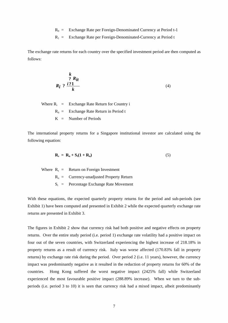
The international property returns for a Singapore institutional investor are calculated using the
following equation:
Rs = Ru + St(1 + Ru) (5)
Where Rs = Return on Foreign Investment
Ru = Currency-unadjusted Property Return
St = Percentage Exchange Rate Movement
With these equations, the expected quarterly property returns for the period and sub-periods (see
Exhibit 1) have been computed and presented in Exhibit 2 while the expected quarterly exchange rate
returns are presented in Exhibit 3.
The figures in Exhibit 2 show that currency risk had both positive and negative effects on property
returns. Over the entire study period (i.e. period 1) exchange rate volatility had a positive impact on
four out of the seven countries, with Switzerland experiencing the highest increase of 218.18% in
property returns as a result of currency risk. Italy was worse affected (170.83% fall in property
returns) by exchange rate risk during the period. Over period 2 (i.e. 11 years), however, the currency
impact was predominantly negative as it resulted in the reduction of property returns for 60% of the
countries. Hong Kong suffered the worst negative impact (2425% fall) while Switzerland
experienced the most favourable positive impact (288.89% increase). When we turn to the sub-
periods (i.e. period 3 to 10) it is seen that currency risk had a mixed impact, albeit predominantly
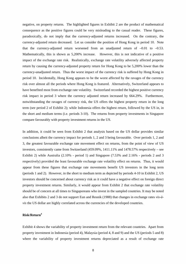
8
negative, on property returns. The highlighted figures in Exhibit 2 are the product of mathematical
consequence as the positive figures could be very misleading to the casual reader. These figures,
paradoxically, do not imply that the currency-adjusted returns increased. On the contrary, the
currency-adjusted return decreased. Let us consider the position of Hong Kong in period 10. Note
that the currency-adjusted return worsened from an unadjusted return of –0.01 to –0.53.
Mathematically, this is shown as 5,200% increase. However, this is not indicative of a positive
impact of the exchange rate risk. Realistically, exchange rate volatility adversely affected property
return by causing the currency-adjusted property return for Hong Kong to be 5,200% lower than the
currency-unadjusted return. Thus the worst impact of the currency risk is suffered by Hong Kong in
period 10. Incidentally, Hong Kong appears to be the worst affected by the ravages of the currency
risk over almost all the periods where Hong Kong is featured. Alternatively, Switzerland appears to
have benefited most from exchange rate volatility. Switzerland recorded the highest positive currency
risk impact in period 3 where the currency adjusted return increased by 664.29%. Furthermore,
notwithstanding the ravages of currency risk, the US offers the highest property return in the long
term (see period 2 of Exhibit 2); while Indonesia offers the highest return, followed by the US in, in
the short and medium terms (i.e. periods 3-10). The returns from property investments in Singapore
compare favourably with property investment returns in the US.
In addition, it could be seen from Exhibit 2 that analysis based on the US dollar provides similar
conclusions albeit the currency impact for periods 1, 2 and 3 being favourable. Over periods 1, 2 and
3, the greatest favourable exchange rate movement effect on returns, from the point of view of US
investors, consistently came from Switzerland (459.09%, 1411.11% and 1478.57% respectively – see
Exhibit 2) while Australia (2.10% - period 1) and Singapore (7.53% and 2.16% - periods 2 and 3
respectively) provided the least favourable exchange rate volatility effect on returns. Thus, it would
appear from these figures that exchange rate movements benefit US investors in the long term
(periods 1 and 2). However, in the short to medium term as depicted by periods 4-10 in Exhibit 2, US
investors should be concerned about currency risk as it could have a negative effect on foreign direct
property investment returns. Similarly, it would appear from Exhibit 2 that exchange rate volatility
should be of concern at all times to Singaporeans who invest in the sampled countries. It may be noted
also that Exhibits 2 and 3 do not support Eun and Resnik (1988) that changes in exchange rates vis-à-
vis the US dollar are highly correlated across the currencies of the developed countries.
Risk/Return4
Exhibit 4 shows the variability of property investment return from the relevant countries. Apart from
property investment in Indonesia (period 4), Malaysia (period 4, 8 and 9) and the US (periods 5 and 8)
where the variability of property investment returns depreciated as a result of exchange rate
9
movements to imply negative correlation of property and exchange rate returns (see Exhibit 4),
exchange rate volatility predominantly aggravated the risk for property investment in every country
and period. The variability of property returns attendant to exchange rate fluctuations increased by
113.43% (Australia) to 442.27% (Germany) for period 1, and by 32.34% (US) to 3,050% (Hong
Kong) for period 2. France, with 13,050% inflation in risk in period 6 (see also Addae-Dapaah and
Goh, 1998: 73), experienced the highest increase in the variability of property returns as a result of
currency volatility. Thus, the figures in Exhibit 4 imply a positive correlation of property foreign
currency returns and the corresponding foreign exchange returns. Furthermore, Exhibit 4 supports
Ziobrowski and Ziobrowski (1995) that assets with low domestic risk seem to be more susceptible to
international exchange rate correlation than assets with high domestic risk. This could, however, be a
function of the scale problem.
It may be noted that Indonesia and Malaysia have the highest risk (as measured by standard deviation)
in almost every period where they are included in the analysis (see Exhibit 4). This relatively high
risk could be a function of the recent South East Asia currency crisis, which severely affected the
economies of both countries. Notwithstanding the ravages of the currency crisis, Indonesia and
Malaysia have the lowest risk in terms of coefficient of variation (see Exhibit 5). It would appear
that, on the basis of coefficient of variation, the US generally is the safest (see Exhibit 5) for a
Singapore investor. Furthermore, similar conclusions are replicated when the analyses are based on
the US dollar (see Exhibit 4) – i.e. that exchange rate fluctuations generally exacerbate property return
variability. Exhibits 6a & b provide a brief comparison of the variability of property foreign currency
return as a function of the Singapore, and the US dollar. It may be safely concluded from Exhibits 4
and 6a & b that similar analyses for any country would produce similar variability relative to that
country’s exchange rate volatility.
Correlation Coefficients of Quarterly Property Returns5
The correlation coefficients (and the corresponding p-values) of the sampled data presented in
Appendix 1 (and summarised in Exhibit 7) show that the degree of association between the markets
ranges from –1 to +1. The perfect positive correlations (period 10) and the other relatively high
positive correlations (i.e. >0.80) exist among the EU countries while the perfect negative correlations
are between Switzerland and the EU countries. Notwithstanding these extremes of correlation
coefficients, it is evident from Exhibit 7 that the proportion of the correlation coefficients (unadjusted
and adjusted), which is statistically insignificant at 1%,6 is considerably higher than the proportion
that is statistically significant at 1% for all the periods except period one. Furthermore, 17.76% and
14.23% of the unadjusted and adjusted correlation coefficients respectively are negative (see Exhibit
7). All these imply that there is a great scope for diversification in the sampled markets. This is
10
reinforced by the fact that most of the correlation coefficients are below 0.5. For example, about 61%
and 71% of the correlation coefficients are lower than 0.5 in periods one and two respectively.
Another important feature to note from the figures in Appendix 1 and Exhibit 7 is the impact of
exchange rate movements on the correlation coefficients. Currency volatility had both positive and
negative effects on the correlations during all the periods. For instance, the correlation between
Singapore and Hong Kong (period 2), and Netherlands and Italy (period 10), changed from +0.1945
to –0.1128, and +1 to –0.9502 (positive impact) respectively after adjusting for currency risk.
Conversely, the correlations between Singapore and Switzerland (period 5), and Netherlands and
Switzerland (period 10) changed from –0.2482 to +0.0578, and –1 to 0.8931 respectively (negative
effect) as a result of exchange rate volatility. An examination of Exhibit 7 reveals that exchange rate
fluctuations increased, and reduced, the proportion of positive correlations that were found to be
significant at 1% for six and three periods respectively. Similarly currency risk reduced the
percentage of the negative correlations that were found to be significant at 1% for five periods and
increased that of four periods.
The net impact of these positive and negative effects, which are a function of the correlation between
exchange rate returns and the correlation between exchange rate returns and foreign currency
denominated property returns (see Exhibit 8), on the return and risk of a portfolio is yet to be
ascertained. A positive correlation between exchange rate, and unadjusted property, returns suggests
that hedging always reduces risk while a negative correlation implies the possibility that hedging
increases rather than reduces risk (Benari, 1991). This can be explained by the following formula:
*2** 2222 ??? ssfft WWV ?? ? fs s*f*sW*fW* ?? (6)
where Vt = total risk of foreign property investment
? f ? s = standard deviation of exchange rates and property returns respectively
WfWs = proportion of exchange rates and property returns
? = correlation between exchange rate and property returns
Thus total portfolio risk will decrease when the correlation between the two elements is negative.
Hedging, in such a situation, will restrict or forestall the risk reduction attendant to the negative
correlation. Alternatively, since a positive correlation between exchange rate and property returns
increases the portfolio risk, hedging in such instances, will reduce the risk of foreign property
investment. Exhibit 8 shows that apart from France (period 6), Switzerland (periods 9 & 10),
Indonesia (period 10) and Japan (period 8), all the positive correlations are relatively low (i.e. <0.5).
11
This implies that the cost of hedging, if undertaken, may erode the benefits of enhanced return and
reduced risk (see Dawson and Rodney, 1994). It may further be noted that Italy is the only market
with a positive correlation, albeit relatively low, for every period while Germany has a negative
correlation for nine out of ten periods (see Exhibit 8). The inter-country correlations, especially the
currency adjusted correlations (Appendix 1), do not provide evidence of convergence of the markets
of the developed countries (apart from the EU markets) due to greater economic synchronization as
suggested by Errunza (1977, 1983).
In addition, it could be seen from Appendix 2 that apart from period 5 (i.e. 92-94/95-6 in Appendix 2)
where the correlations are relatively unstable, the inter country correlation coefficients for the
remaining periods are relatively stable over time at a 5% level of significance.
Significance Testing of Effect(s) of Currency Risk
We aim, at this juncture, to ascertain the statistical significance of the impact of exchange rate
volatility demonstrated by Exhibits 2, 3 and 5. To do this, we have employed z-statistic,7 t-statistic,8
and a Fisher transformation9 (see Myers and Well [1991]) to test the null hypothesis that there is no
difference between the currency-adjusted and unadjusted mean returns, standard deviation (risk) and
correlation coefficients. The t-statistic is used for periods 6 to 10 of Appendix 3 where the sample
size is relatively small (i.e. N ? 12). The null hypothesis is rejected if the test-statistic for the t-
statistic two-tailed test at a 5% significance level falls into the critical region of >+2.064 or <-2.064.
Similarly, a two-tailed z-statistic at 5% significance level will reject the null hypothesis if the test
statistic falls into the critical region of >+1.96 or <-1.96. The results of the hypothesis testing are
presented in Appendices 3 and 4. Apart from Hong Kong (period 6 of Appendix 3) where the impact
of currency risk is significant, Appendix 3 implies that the effect of exchange rate movement on
return and risk is virtually statistically insignificant for all the sampled countries over all the periods.
Unfortunately, however, currency movements have a mixed impact on the correlation coefficients.
Figures in Appendix 4 reveal that there are statistically significant exchange rate volatility effects on
the correlations, especially for periods 6 to 8. This implies that anyone whose investment horizon is ?
3 years should be mindful of the effects of currency risk on the correlation of returns. However, it
may be argued that since international direct property investment generally is a medium to long-term
investment, most investors would not be affected by the short-term effect(s) of currency risk on the
correlation of returns.
12
Currency volatility generally has statistically insignificant impact on the correlation of returns for the
long and medium terms (i.e. periods 1 to 5). Only about 12% of the correlations for periods 1 to 5 are
statistically significantly affected by currency risk. It must be noted that 37% of the statistically
significant effect is positive – i.e. currency risk either changes a hitherto positive correlation to
negative, or considerably reduces the magnitude of a positive correlation. Such an effect will cause
the efficient frontier to move to the left, thus reducing portfolio risk and enhancing return. This
means that exchange rate fluctuations adversely affect only 7.6% of the correlation of returns for the
long and medium terms (i.e. periods 1 to 5). Thus the inclusion of any of the combinations of the
countries with adverse statistically significant currency risk effect in a portfolio will cause the
efficient frontier to move to the right to increase the risk of the portfolio and reduce return. The
inclusion of Germany-Netherlands (in particular) in a portfolio of direct property investment could be
potentially disastrous as the negative exchange rate volatility effect is statistically significant for the
correlations of all the periods except periods 8 and 9 (see Appendix 4).
Optimal Portfolio
The main goal is creating an efficient portfolio of direct property investment from the sampled
countries without allowing for short selling. The expected return on the portfolio is the weightage
average returns of direct property investment for each country.
Mathematically ??
?n
iiRiWpR
1 (7)
where ??
n
iiW
1 = 1
Rp = the expected return on portfolio p
Wi = the proportions of direct property investment of the country in the total
portfolio
Ri = the expected return on asset i
n = the number of assets in the portfolio
Similarly the portfolio risk is the weighted average of the variability and the correlation coefficient of
the returns from the sampled countries. In the mathematical notation,
13
??
?
??
??
??n
1ijWiW
)ji(
n
1i
n
1j22
i2iW2
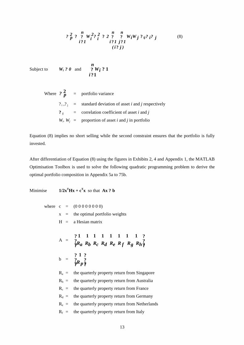
p ?? ? ij ji?? (8)
Subject to Wi ? 0 and ??
?n
iiW
11
Where 2p? = portfolio variance
? i ,? j = standard deviation of asset i and j respectively
? ij = correlation coefficient of asset i and j
Wi. Wj = proportion of asset i and j in portfolio
Equation (8) implies no short selling while the second constraint ensures that the portfolio is fully
invested.
After differentiation of Equation (8) using the figures in Exhibits 2, 4 and Appendix 1, the MATLAB
Optimisation Toolbox is used to solve the following quadratic programming problem to derive the
optimal portfolio composition in Appendix 5a to 75b.
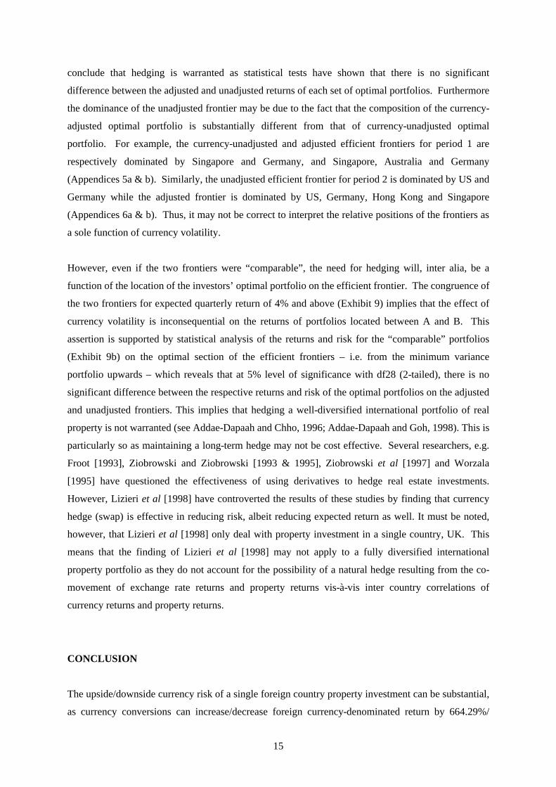
Minimise 1/2xTHx + cTx so that Ax ? b
where c = (0 0 0 0 0 0 0 0)
x = the optimal portfolio weights
H = a Hesian matrix
A = ???
?
???
?
hRgRfReRdRcRbRaR11111111
b = ???
?
???
?
pR1
Ra = the quarterly property return from Singapore
Rb = the quarterly property return from Australia
Rc = the quarterly property return from France
Rd = the quarterly property return from Germany
Re = the quarterly property return from Netherlands
Rf = the quarterly property return from Italy
14
Rg = the quarterly property return from Spain
Rh = the quarterly property return from Switzerland
Rp = the expected portfolio return
Each optimal portfolio minimises the portfolio’s risk without allowing for short selling and riskless
lending and borrowing (Elton and Gruber [1994]). The expected return figures in Appendix 5a to 7b
do not vary at constant intervals because of the above constraints.
It is worth noting that the composition of the currency-unadjusted optimal portfolio differs from that
of the currency-adjusted optimal portfolio for each of the periods (see Appendices 5a – 7b). For
example, Australia plays a very minor role in the currency-unadjusted optimal portfolio (see
Appendix 5a) but a dominant role in the currency-adjusted optimal portfolio (see Appendix 5b).
Similarly, the composition of the currency-unadjusted optimal portfolio for period 2 implies that there
should be no investment in Singapore whereas Singapore is fairly represented in the currency-adjusted
optimal portfolio for the period (see Appendices 6a & b). The US dominates the optimal portfolio
composition for period 2 (Appendices 6a & b). The surprisingly striking feature about the optimal
portfolio composition for period 4 (Appendices 7a & b) is the dominance of the Far Eastern countries,
especially, Indonesia.
Notwithstanding the different composition of the currency-unadjusted and adjusted optimal portfolios,
a “means test” at the 5% level of significance reveals that there is no significant difference between
the “means” of the respective return and standard deviation for each pair of optimal portfolios (i.e. for
periods 1, 2 and 4 respectively).
Efficient frontiers (Exhibits 9 to 11) are constructed from the expected return and portfolio risk
figures in Appendices 5a to 7b. Exhibit 9 (period 1) shows that, at a standard deviation of 9.70%, a
100% property investment in Singapore is as good as a fully diversified portfolio. However, a 100%
property investment in the US (with a standard deviation of 3.56%), and in Indonesia (with a standard
deviation of 20.50%) is as good as a fully diversified portfolio during periods 2 (i.e. Exhibit 10) and 4
(Exhibit 11) respectively. This discrepancy is a function of the difference in the optimal portfolio
composition for the periods.
Furthermore, an examination of Exhibits 9-11 reveals that the currency-adjusted and unadjusted
frontiers are either congruent or tangential, or that the currency-unadjusted frontier dominates the
currency-adjusted frontier. In some instances, e.g. Exhibit 9, the gap between the currency-adjusted
and unadjusted frontiers is as wide as three standard deviations. This may generally portend the need
to hedge returns against the ravages of currency movements. However, it may not be prudent to
15
conclude that hedging is warranted as statistical tests have shown that there is no significant
difference between the adjusted and unadjusted returns of each set of optimal portfolios. Furthermore
the dominance of the unadjusted frontier may be due to the fact that the composition of the currency-
adjusted optimal portfolio is substantially different from that of currency-unadjusted optimal
portfolio. For example, the currency-unadjusted and adjusted efficient frontiers for period 1 are
respectively dominated by Singapore and Germany, and Singapore, Australia and Germany
(Appendices 5a & b). Similarly, the unadjusted efficient frontier for period 2 is dominated by US and
Germany while the adjusted frontier is dominated by US, Germany, Hong Kong and Singapore
(Appendices 6a & b). Thus, it may not be correct to interpret the relative positions of the frontiers as
a sole function of currency volatility.
However, even if the two frontiers were “comparable”, the need for hedging will, inter alia, be a
function of the location of the investors’ optimal portfolio on the efficient frontier. The congruence of
the two frontiers for expected quarterly return of 4% and above (Exhibit 9) implies that the effect of
currency volatility is inconsequential on the returns of portfolios located between A and B. This
assertion is supported by statistical analysis of the returns and risk for the “comparable” portfolios
(Exhibit 9b) on the optimal section of the efficient frontiers – i.e. from the minimum variance
portfolio upwards – which reveals that at 5% level of significance with df28 (2-tailed), there is no
significant difference between the respective returns and risk of the optimal portfolios on the adjusted
and unadjusted frontiers. This implies that hedging a well-diversified international portfolio of real
property is not warranted (see Addae-Dapaah and Chho, 1996; Addae-Dapaah and Goh, 1998). This is
particularly so as maintaining a long-term hedge may not be cost effective. Several researchers, e.g.
Froot [1993], Ziobrowski and Ziobrowski [1993 & 1995], Ziobrowski et al [1997] and Worzala
[1995] have questioned the effectiveness of using derivatives to hedge real estate investments.
However, Lizieri et al [1998] have controverted the results of these studies by finding that currency
hedge (swap) is effective in reducing risk, albeit reducing expected return as well. It must be noted,
however, that Lizieri et al [1998] only deal with property investment in a single country, UK. This
means that the finding of Lizieri et al [1998] may not apply to a fully diversified international
property portfolio as they do not account for the possibility of a natural hedge resulting from the co-
movement of exchange rate returns and property returns vis-à-vis inter country correlations of
currency returns and property returns.
CONCLUSION
The upside/downside currency risk of a single foreign country property investment can be substantial,
as currency conversions can increase/decrease foreign currency-denominated return by 664.29%/
16
5,200% (see Exhibit 2, periods 3 & 10) and attenuate/amplify risk by 17.6%/13,050% (see Exhibit 4,
periods 8 & 6). This is consistent with the findings of Addae-Dapaah and Goh [1998], Worzala
[1995], Radcliffe [1994], and Ziobrowski and Curcio [1991]. However, hypotheses tests at 5% level
of significance reveal that apart from Hong Kong, the impact of the exchange rate volatility on return
and risk is virtually statistically insignificant.
Exhibits 9 to 11 depict the cumulative impact of exchange rates movement. The Exhibits show that
the currency-unadjusted and adjusted frontiers are either congruent or tangential, or that the
unadjusted frontiers dominate the adjusted frontiers. The difference between the two frontiers is not,
however, statistically significant at 5% level of significance. This is a function of the relatively low
correlations, and even negative correlations between exchange rate returns and unadjusted property
returns vis-à-vis the relatively low positive and negative inter-country correlations of exchange rate
returns and property returns, which enable movements between the currency returns and a fully
diversified international property portfolio return over time to provide a natural hedge against
currency movement. Therefore, the hypothesis that currency risk has a significant effect on the return
from a fully diversified international property portfolio is rejected.
Since the difference between the mean returns of the unadjusted and adjusted optimal portfolios is not
large enough to be significant from a practical business perspective, investors with fully diversified
international property portfolios should not be unduly apprehensive of the ravages of currency risk.
Furthermore, it must be noted that the composition of the currency-adjusted optimal portfolio differs
from that of the unadjusted optimal portfolio (see Appendix 5-7). However, the difference between
the unadjusted and the adjusted optimal portfolio returns has been found to be insignificant from any
practical business perspective to imply that hedging of a well-diversified portfolio of international real
estate investment is not a necessity.
NOTES
1 This assumption is necessary to ensure that subsequent analyses and conclusions are neither
complicated by, nor tainted with, capital rationing issues. 2 Matlab is computer software developed and patented by Mathworks, Inc. (1998), Latik,
Massachusetts, USA. The software has both a PC version and an Unix version. Matlab has several toolboxes including the Optimisation toolbox, which was employed for the computation of the optimal portfolio for this paper. By following the instructions and steps in the toolbox, entering the relevant data, and typing the command: X=qp(H,C,A,b,vlb,vub,xO,neqcstr) – see Matlab Toolbox Manual – the software will compute and give you the optimal portfolio weightages. By typing another command:
½ * ?’ * H * ? (see Matlab Toolbox Manual)

17
The portfolio variance for the specific expected return will be given. 3 Expected (rate of) return is used in this paper because the analyses and conclusions are based on
the arithmetic mean of historic quarterly return data. Since a mean has a measure of variability (i.e. risk), and the future is also uncertain, the term “expected” (rate of) return is used to reflect the element of uncertainty.
4 Following the notations in the paper, the risk for foreign currency denominated return is calculated
as follows:
k
k
tiRitR?
??
? 1
2)(
?
where ? = standard deviation of asset; while the total risk for currency adjusted return is calculated as follows:
xiixs ???? 222 ???
where 2x? and 2
i? are the variance of exchange rate return, and return on asset i
respectively. 5 The correlation coefficients re calculated as follows:
ji
jiCovij ??
?),(
?
subject to –1 ? ? ij ? 1
??
??n
jijRjRiRiR
njiCov
1,)*)(*(
1),(
where ? ij = correlation coefficient between asset i and j Cov(i,j) = covariance between asset i and j Ri, Rj = actual return on asset i and j respectively
?*jR,*
iR expected return on asset i and j respectively
? i , ? j = standard deviation of asset i and j respectively n = number of equally likely joint outcomes The adjusted correlation coefficients are based on the currency adjusted returns and standard
deviations.
18
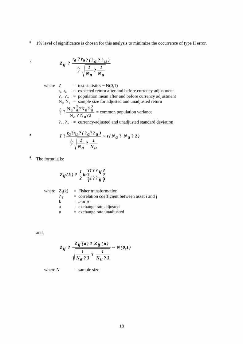
6 1% level of significance is chosen for this analysis to minimize the occurrence of type II error.
7
uN1
nN1^
)ua(urarijZ
?
????
?
??
where Z = test statistics ~ N(0,1) ra, ru = expected return after and before currency adjustment ? a, ? u = population mean after and before currency adjustment Na, Nu = sample size for adjusted and unadjusted return
2uNaN
2uuN2
aaN^?????
?? = common population variance
? a, ? u = currency-adjusted and unadjusted standard deviation
8 )2uNaN(t~
uN1
aN1^
)ua(urarT ??
?
????
?
??
9 The formula is:
???
?
???
?
?
??
ij1ij1
ln21
)k(ijZ?
?
where Zij(k) = Fisher transformation ? ij = correlation coefficient between asset i and j k = a or u a = exchange rate adjusted u = exchange rate unadjusted and,
)1,0(N~
3uN1
3aN1
)u(ijZ)a(ijZijZ
??
?
??
where N = sample size
19
Reference:
Addae-Dapaah, K. and B.K. Choo, International Diversification of Property Stock – A Singaporean Investor’s Viewpoint, Real Estate Finance, Fall 1996, 13:3, 54-66. Addae-Dapaah, K. and L.Y. Goh, Currency Risk and Office Investment in Asia Pacific, Real Estate Finance, Fall 1998, 15:3, 67-85. Balogh, C. and J. Sultan, Investing in Foreign Real Estate: A Primer, Real Estate Review, Spring 1997, 7:1, 73-80. Benari, Y., When is Hedging Foreign Assets Effective? Journal of Portfolio Management, Fall 1991, 18:1, 66-71. Boydell, S. and P. Clayton, Property as an Investment Medium: Its Role in the Institutional Portfolio. London: Financial Times Business Information, 1992. Brueggeman, W.B., A.H. Chen, and T.G. Thibodeau, Real Estate Investment Funds: Performance and Portfolio Considerations, Journal of American Real Estate and Urban Economics Association, 1984, 12, 333-354. Dawson, A. and W.H. Rodley, The Use of Exchange-Rate Hedging Techniques by UK Property Companies, Journal of Property Finance, 1994, 4:5, 56-67. Elton, E.J. and M.J. Gruber, Modern Portfolio Theory and Investment Analysis, New York: John Wiley & Sons, 4th Edition, 1994. Errunza, V.R., Gains from Portfolio Diversification into Less Developed Countries Securities, Journal of International Business Studies, Fall/Winter 1977, 8:2, 83-99. ___________ Emerging Markets: A New Opportunity for Improving Global Portfolio Performance, Financial Analyst Journal, September/October 1983, 39:5, 51-58. Eun, C.S. and B.G. Resnick, Exchange Rate Uncertainty, Forward Contracts, and International Portfolio Selection, Journal of Finance, March 1988, 43:1, 197-215. Firstenberg, P.M., S.A. Ross, and R.M. Zisler, Real Estate: The Whole Story, Journal of Portfolio Management, Spring 1988, 14:3,23-32. Fraser, W., The Risk of Property to the Institutional Investor, Journal of Valuation, 1985,4:1, 45-49. Friedman, H.S., Real Estate Investment and Portfolio Theory, Journal of Financial and Quantitative Analysis, 1970, 5, 861-874. Froot, K.A., Currency Hedging Over Long Horizons, Working Paper Series, National Bureau of Economic Research, 1993. Lessard, D.R., International Portfolio Diversification: A Multivariate Analysis for a Group of Latin-American Countries, Journal of Finance, June 1973, 28:3, 619 –633. Lessard, D.R., World, Country and Industry Relationships in Equity Returns, Financial Analysts Journal,January-February, 1976, 32:1, 32-38.
20
Levin, J. and A.D. Fox, Elementary Statistics in Social Research, New York: Harper Collins Publishers, 1991. Levy, H. and M. Sarnat, International Diversification of Investment Portfolios, American Economic Review, 1970, 60, 668-675. Liow, K.H., Property Policy, Property Asset Values and Share Prices for Property Intensive Companies, Unpublished Ph.D. thesis, University of Manchester (1994). Lizieri, C. and L. Findlay, International Property Portfolio Strategies: Problems and Opportunities, Journal of Property Valuation and Investment, 1995, 13: 1, 6-21. Lizieri, C, E. Worzala, and , R.Johnson , To Hedge or Not to Hedge? A study of international real estate investment under exchange rate uncertainty, London: The Royal Institution of Chartered Surveyors, 1998. Logue, D.E. An Experiment in International Diversification, Journal of Portfolio Management, Fall 1982, 8, 22-27. Newell, G. and E. Worzala, The Role of International Property in Investment Portfolio, Journal of Property Finance, 1995, 6:1, 55-63. Panton, D.B., V.P. Lessig, and O.M. Joy, Co-Movement of International Equity Markets: A Taxanomic Approach, Journal of Financial and Quantitative Analysis, September, 1976, 11:3, 415-432. Pellat, P.G.K., The Analysis of Real Estate Investments Under Uncertainty, Journal of Finance, 1972, 27, 459-471. Radcliffe, R.C. Investment: Concepts, Analysis, Strategy. New York: Harper Collins College Publishers, 4th Edition, 1994. Roulac, S.E., Can Real Estate Returns Outperform Common Stocks? Journal of Portfolio Management, 1976, 2, 26-43. Rubens, H.J., T.M. Bond, and R.J. Webb, The Inflation Hedging Effectiveness of Real Estate, Journal of Real Estate Research, Summer 1989, 4:2, 45-54. Solnik, B.H. Why Not Diversify Internationally Rather Than Domestically? Financial Analysts Journal, July-August, 1974, 30:4, 48-54. Solnik, B.H., International Investments, Boston: Addison-Wesley, 3rd Edition, 1996. Taylor, J.H., Global Investing for the 21st Century, Singapore: Toppan, 1995. Webb, J.R. and J.A Rubens, How Much in Real Estate? A Surprising Answer, Journal of Portfolio Management, Spring 1987, 13:3, 10-14. Webb, J.R., R.J. Curcio, and J.H.Rubens, Diversification Gains from Including Real Estate in Mixed-Asset Portfolios, Decision Sciences, 1985, 19, 434-452.
21
Worzala, E., Currency Risk and International Property Investments. Journal of Property Valuation and Investment, 1995,13:5, 23-28. Ziobrowski, A.J. and R.J. Curcio, Diversification Benefits of US Real Estate to Foreign Investors, Journal of Real Estate Research, 1991, 6:2, 119-142. Ziobrowski, A.J. and B.J. Ziobrowski, Hedging Foreign Investments in US Real Estate with Currency Options, Journal of Real Estate Research, 1993, 8:1, 27-54. Ziobrowski, A.J. and B.J. Ziobrowski, Using Forward Contracts to Hedge Foreign Investment in US Real Estate, Journal of Property Valuation and Investment, 1995, 13:1, 22-43. Ziobrowski, A.J., B.J. Ziobrowski and S. Rosenberg, Currency Swaps and International Real Estate Investment, Real Estate Economics, 1997, 25:2, 223-251.