Current Management in a Hybrid Fuel Cell PowerSystem: A Model Predictive Control Approach∗

Ardalan Vahidi † Anna Stefanopoulou Huei PengDepartment of Mechanical Engineering, University of Michigan

Abstract

The problem of oxygen starvation in fuel cells coupled with air compressor sat-uration limits is addressed in this paper. We propose using a hybrid configuration,in which a bank of ultracapacitors supplements the polymer electrolyte membranefuel cell during fast current transients. Our objective is to avoid fuel cell oxygenstarvation, prevent air compressor surge and choke, and simultaneously match anarbitrary level of current demand. We formulate the distribution of current demandbetween the fuel cell and the bank of ultracapacitors in a model predictive controlframework which can handle multiple constraints of the hybrid system. Simulationresults show that reactant deficit during sudden increase in stack current is reducedfrom 50% in stand-alone architecture to less than 1% in the hybrid configuration.In addition the explicit constraint handling capability of the current managementscheme prevents compressor surge and choke and maintains the state-of-charge ofthe ultracapacitor within feasible bounds.

1 IntroductionFuel cells are electrochemical devices that convert the chemical energy of a hydrogen fuelinto electricity through a chemical reaction with oxygen. The byproducts of this chemicalreaction are water and heat. When compressed pure hydrogen is available, the subsystemthat supplies oxygen to the cathode is one of the key controlled components of a fuel cellstack and is the subject of this paper. It is known in the fuel cell community that lowpartial oxygen pressure in the cathode reduces the fuel cell voltage and the generatedpower, and it can reduce the life of the stack. Song et. al. [1] show rapid drop involtage when hydrogen or oxygen starvation occurs in phosphoric acid fuel cells. In apatent filed by Ballard [2] data shows that the fuel cell voltage is reversed during oxygen

∗This work is funded by NSF 0201332 and the Automotive Research Center (ARC) under U.S. Armycontract DAAE07-98-3-0022.

†Corresponding Author, currently at Department of Mechanical Engineering, Clemson University,Clemson, SC 29634, avahidi@clemson.edu

1

starvation. Moreover the temperature within the fuel cell may rapidly increase whenoxygen concentration is too low. Therefore the oxygen should be replenished quicklyas it is depleted in the cathode. In high-pressure fuel cells a compressor is used toprovide the required air into the cathode. The control challenge is that oxygen is depletedinstantaneously when current is drawn from the stack, while the air supply rate is limitedby the supply manifold dynamics and compressor operational constraints [3].

Air compressors can consume up to 30% of the fuel cell power during rapid increasein the air flow. Centrifugal compressors of the type used with high-pressure fuel cells, aresusceptible to surge and choke that limit the efficiency and performance of the compressor[4]. Choke occurs at high mass flows, during step-up in compressor motor commandand surge occurs at low mass flows, normally during a sudden step-down in compressormotor command. Surge is specially critical as it causes undesirable flow oscillations andinstability and it can even result in backflow through the compressor and the installationdownstream of the compressor [5]. Therefore extra measures need to be taken duringstep-down in demand to prevent compressor surge and during step-up to prevent choke.It is shown in [6] that control efforts targeting the compressor have a great potential forimproving system performance.

In [3], it is shown that a combination of feedback and feedforward control of thecompressor input, can improve the transient oxygen response. However the drop in oxygenlevel could not be eliminated by merely relying on compressor control unless the intentionto change the load levels is known in advance. To protect against reactant starvation, Sunand Kolmanovsky [7] propose using a “load governor” which controls the current drawnfrom the fuel cell. The load governor ensures that constraints on oxygen level are fulfilledat the cost of slower fuel cell response to current demand. Air compressor constraintshave not been explicitly addressed in the existing literature on fuel cell power systems.

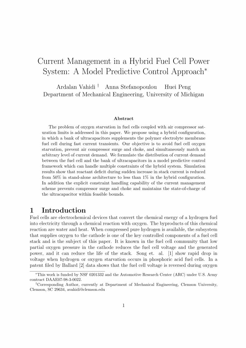
One way to avoid a) fuel cell oxygen starvation b) compressor saturation, and c) simul-taneously match an arbitrary level of current demand, is to add a rechargeable auxiliarycurrent source which can respond quickly to a change in current demand. Splitting thecurrent demand with a battery or an ultracapacitor for example offers additional flexibilityin managing the electric loads. The battery or ultracapacitor can be connected with a fuelcell through a DC/DC converter as shown in Fig. 1. Other configurations of the electricconnection between a fuel cell and an auxiliary energy supply are discussed in [8]. In allcases the auxiliary power source buffers the peaks in demand and can be recharged by thefuel cell itself, when the demand is lower. In this work we use a bank of ultracapacitorsas the auxiliary power source to the fuel cell. We design a current splitting scheme whichminimizes oxygen starvation and ultracapacitor usage while it enforces bounds on ultra-capacitor’s state of charge and prevents compressor surge and choke. The capability toexplicitly handle constraints of the system is the motivation for using a model predictivecontrol (MPC) approach in this problem.

The requirements for the supervisory controller formulated here are therefore differentfrom those of existing power management schemes for hybrid vehicles. Most supervisorypower split methods aim to minimize fuel consumption and enforce constraints of state

2

Load

UltraCapacitor

Model Predictive Control Module

Ifc

vcm

S

HydrogenTank

Compressor

Motor

Icap

DC/DCConverter

Power Bus

Ifc

Delivered

Ides

Figure 1: Schematic of the hybrid fuel cell control system. The fuel cell stack consists of 350 cells withpeak power of 75 kW. The high pressure air supply is powered by a 12 kW compressor. A small auxiliarypower source provides additional power when needed.

of charge of the auxiliary power source. Due to their emphasis in fuel consumption overa typical loading cycle the prior work can be categorized as: (i) “Rule-based” in whichpower splitting is based on instant demand [9, 10]. The advantage of these methods istheir relative simplicity. However these methods cannot take into account simultaneousconstraints in the interacting subsystems (ii) “Optimization-based” methods on the otherhand, optimize the overall system performance over a decision horizon and can accountfor subsystem constraints. Dynamic programming (DP) is one of the optimization-basedapproaches that has been used for power management of hybrid electric vehicles. Inmost scenarios dynamic programming is used offline for a given load cycle and thereforeis cycle specific [11, 12]. While most of these schemes are designed for hybrids withinternal combustion engines, they can be applied to hybrids of fuel-cell with batteries orultra-capacitors for vehicle [13, 14] or other applications [15]. Guezennec et al. [16] usea heuristic approach called “equivalent consumption minimization strategy” for powermanagement of a fuel cell hybrid, which minimizes hydrogen consumption and regulatesstate of charge of the auxiliary power source. Rodatz et al. have used an optimal controldesign to minimize the hydrogen consumption in a hybrid fuel cell system [17]. Theirdesign ensures that the auxiliary power source is charged at the end of each cycle.

The MPC controller that we formulate in this paper satisfies upper and lower boundson the state of charge of the auxiliary power source and compressor constraints at allinstances. Figure 1 shows the schematic of a fuel cell stack, the air compressor, a DC/DCconvertor and the model predictive controller, which acts as the supervisory controller.The MPC unit determines the current drawn from the fuel cell (Ifc) and the compressormotor input (vcm) to meet the control design specifications. In our model and problemformulation we assume that a lower level controller in the DC/DC convertor ensures thatIfc is drawn from the fuel cell [8], while the BUS voltage is regulated by the ultracapaci-

3

tor. This work is unique to our knowledge in that it takes into account compressor flowconstraints in the supervisory control design stage. Inclusion of a more realistic ultraca-pacitor model and the compressor surge constraint in this paper are the major additionsto our preliminary results presented in [18]. The

contributions

of this paper

with

reference to

our earlier

ACC paper are

briefly

highlighted

here now.

The next section describes the dynamic model of the fuel cell system followed by adescription of the hybrid system architecture. Model predictive control formulation isbriefly discussed in Sec. 4. In Sec. 5 we explain choice of prediction horizon and penaltyweights, followed by nonlinear simulation results. Conclusions are given in Sec. 6.

2 Model of the Fuel Cell SystemA nonlinear spatially-averaged model of a 75kW fuel cell stack together with its auxiliariesis developed in [19] based on electrochemical, thermodynamic and fluid flow principles.The fuel cell has 350 cells and can provide up to 300 A of current. The model, representingmembrane hydration, anode and cathode flow and stack voltage, is augmented with themodels of ancillary subsystems including the compressor, cooling system and the humidi-fier to obtain a nonlinear model of the overall fuel cell system. We assume that humidity Based on a

comment by

reviewer 3, a

statement is

added here to

highlight the

assumption

that we have

made in the

fuel cell

model.

and temperature are regulated to their desired levels and do not consider the effect oftemperature or humidity fluctuations. This assumption should not limit the validity ofour results since the temperature and humidity dynamics are considerably slower than thefuel cell power dynamics which we study in this paper. We have also assumed that a fastPI controller regulates the hydrogen flow to the anode to match the oxygen flow. Sincethe hydrogen is supplied from a compressed tank, a steady and timely hydrogen supply isassumed. The fuel cell model used in this work is identical to the one in [19, 20] and usedin [3]. Note here that we do not use model simplifications used in [7, 21, 22]. Since thefocus of this paper is on control of air flow, we present the governing equations, essentialto understanding the dynamics between the compressor and the air flow into the cath-ode. The compressor flow, pressure, temperature and power characteristics are modelledusing manufacturer maps [19, 20] and shown also in this section. For completeness, allthe governing equations of this model are listed in the Appendix and consequently someequations appear twice; once in the main paper body and once in the Appendix.

To model the concentration of oxygen in the cathode, we first define a parameter calledoxygen excess ratio λO2 :

λO2 =WO2,in

WO2,rct

, (1)

where WO2,in is the flow of oxygen into the cathode and WO2,rct is the mass of oxygenreacted in the cathode. Low values of λO2 indicate low oxygen concentration in thecathode or oxygen starvation. The rate of oxygen reacted WO2,rct, depends on the currentdrawn from the stack Ifc:

WO2,rct = MO2

nIfc

4F, (2)

where n is the number of cells in the stack, F is the Faraday number, and MO2 is the

4

oxygen molar mass. Therefore if the rate of air supply to the cathode is kept constant,λO2 decreases as more current is drawn from the stack. To maintain the level of oxygenexcess ratio, more air should be supplied to the fuel cell. The flow rate of the oxygen intothe stack WO2,in, is a function of the air flow out of the supply manifold Wsm:

WO2,in = yO2

1

1 + Ωatm

Wsm, (3)

where yO2 = 0.21MO2

Matma

is the mass ratio of oxygen in the dry atmospheric air and Ωatm isthe humidity ratio of the atmospheric air. The mass flow rate out of the supply manifoldWsm, depends on the downstream (cathode) pressure and upstream (supply manifold)pressure psm, through the orifice equation (A16). The total cathode pressure (A11) de-pends on the partial pressure of the (i) oxygen which is supplied WO2,in (A18), oxygenwhich is reacted WO2,rct (A26), and the oxygen removed WO2,out (A23), (ii) nitrogen whichis supplied (A19) and removed (A24) and (iii) the water which is supplied (A20), gener-ated (A28), transported through the membrane (A29) and removed (A25). The additionalcathode states of oxygen mass mO2 (A1), nitrogen mass mN2 (A2), water vapor mass mw,ca

(A3), total return manifold pressure prm (A7), and anode states of hydrogen mass mH2

(A8), and water vapor mw,an (A9), are needed to capture the temporal dynamics of thetotal cathode pressure during a step change in current. The derivation and physical in-terpretation of these equations are omitted here but can be found in [19]. However, toallow the reader understand how the control input affects the supply manifold flow Wsm

and consequently the oxygen flow WO2,in, we add the following relations. Specifically thesupply manifold pressure psm, and mass msm, are related to the compressor’s air flow Wcp,and temperature Tcp, through the following dynamics:

dpsm

dt= Ksm(WcpTcp −WsmTsm), (4)

dmsm

dt= Wcp −Wsm, (5)

where Ksm is a coefficient determined by air specific heat coefficients and the supplymanifold volume. The supply manifold temperature Tsm is defined by the ideal gas law(A14).

The compressor air flow Wcp and its temperature Tcp are determined using a nonlinearmodel for the compressor which has been developed in [19] for an Allied Signals centrifugalcompressor that has been used in a fuel cell vehicle [23].

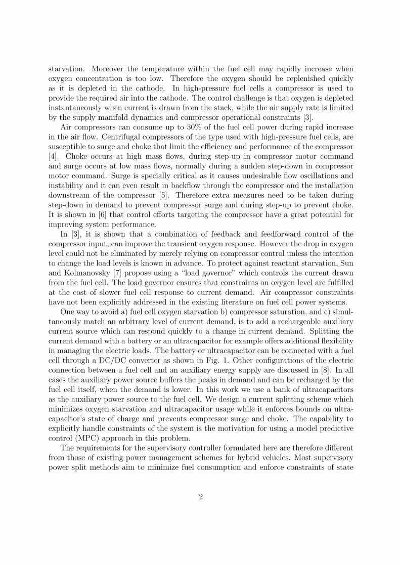
The compressor air mass flow rate Wcp is determined as a function of pressure ratioacross the compressor and blade speed, using a compressor map shown in Figure 2. In thismap, the dashed lines represent boundaries beyond which compressor surge and choke canoccur. The equations used here to represent compressor dynamics are valid within thesebounds. Later in this paper we enforce point-wise-in-time constraints to ensure operationof the compressor inside the bounded region and away from the surge and choke regions.

5

0 0.01 0.02 0.03 0.04 0.05 0.06 0.07 0.08 0.09 0.10.5

1

1.5

2

2.5

3

3.5

4

Corrected Compressor Flow (kg/sec)

Pres

sure

Rat

io (

p sm/p

atm

)

Surge Boundary

Choke Boundary

psm

/patm

≥ 50 Wcp

−0.1

psm

/patm

≤ 15.27 Wcp

+0.6 10 krpm

30 krpm

50 krpm

70 krpm

90 krpm

Corrected Compressor Speed=105 krpm

Figure 2: The compressor map

In our simulations this map is modelled using a nonlinear curve-fitting technique, whichcalculates compressor air flow as a function of inlet pressure patm, outlet pressures psm

and compressor rotational speed ωcp:

Wcp = f(psm

patm

, ωcp) (6)

The details of compressor flow calculation are shown in equation (A34)-(A43) in theAppendix. The compressor outlet temperature and the torque required to drive the com-pressor are calculated using standard thermodynamic equations [24, 25]. The temperatureof the air leaving the compressor is calculated as follows:

Tcp = Tatm +Tatm

ηcp

[(psm

patm

) γ−1γ

− 1

](7)

where γ = 1.4 is the ratio of the specific heats of air, ηcp is the compressor efficiency andTatm is the atmospheric temperature. The compressor driving torque τcp is:

τcp =Cp

ωcp

Tatm

ηcp

[(psm

patm

) γ−1γ

− 1

]Wcp (8)

where Cp is the specific heat capacity of air. The compressor rotational speed ωcp isdetermined as a function of compressor motor torque τcm and the torque required to drivethe compressor τcp:

Jcpdωcp

dt= τcm − τcp (9)

6

0 5 10 15 20 25 30

100

150

200

250

300

Cur

rent

(A

mps

)

0 5 10 15 20 25 30

100

150

200

250

Com

pres

sor

Com

man

d (v

olts

)

0 5 10 15 20 25 300.02

0.04

0.06

0.08

0.1

Com

pres

sor

Flow

(K

g/Se

c)

0 5 10 15 20 25 301.4

1.6

1.8

2

2.2

Oxy

gen

Exc

ess

Rat

io

Time (seconds)

0 5 10 15 20 25 301

2

3

4

Man

ifol

d Pr

essu

re

(bar

)

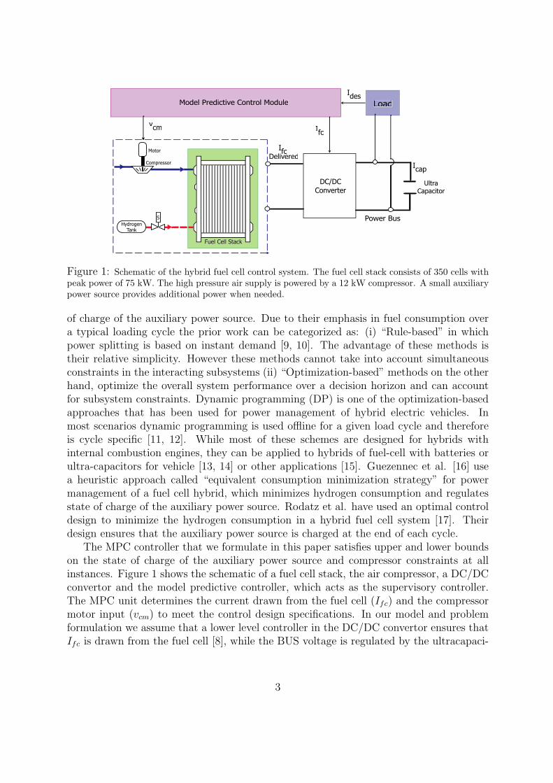
Figure 3: The fuel cell response to step changes in current demand.

where Jcp is the compressor inertia. The compressor motor torque τcm is calculated as afunction of motor voltage vcm using a DC motor model:

τcm = ηcmkt

Rcm

(vcm − kvωcm) (10)

where kt, Rcm and kv are motor constant and ηcm is the motor mechanical efficiency.In summary, the compressor voltage vcm, controls the speed of the compressor through

the first-order dynamics shown in (9) and (10). The speed of the compressor determinesthe compressor flow rate Wcp, which then according to equation (4), affects the supplymanifold pressure psm. The latter, together with the cathode pressure, determines thesupply manifold flow Wsm, and the flow rate of the oxygen into the cathode WO2,in whichfinally affects the excess ratio λO2 given in equation (1).

7

0 0.01 0.02 0.03 0.04 0.05 0.06 0.07 0.08 0.09 0.10.5

1

1.5

2

2.5

3

3.5

4

Flow (kg/sec)

Pres

sure

Rat

io

0 5 10 15 20 25 30100

200

300

Cur

rent

Time (sec)

t=3

t=6

t=9

t=12

t=15

t=18

t=21

t=24

t=27

t=30 seconds

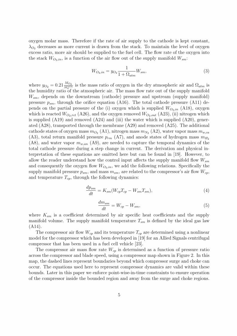
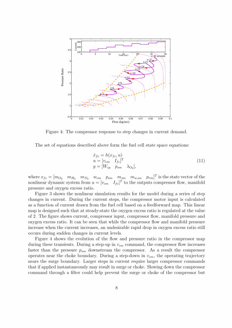
Figure 4: The compressor response to step changes in current demand.

The set of equations described above form the fuel cell state space equations:

xfc = h(xfc, u)u = [vcm Ifc]

T

y = [Wcp psm λO2 ],(11)

where xfc = [mO2 mH2 mN2 wcm psm msm mw,an prm]T is the state vector of thenonlinear dynamic system from u = [vcm Ifc]

T to the outputs compressor flow, manifoldpressure and oxygen excess ratio.

Figure 3 shows the nonlinear simulation results for the model during a series of stepchanges in current. During the current steps, the compressor motor input is calculatedas a function of current drawn from the fuel cell based on a feedforward map. This linearmap is designed such that at steady-state the oxygen excess ratio is regulated at the valueof 2. The figure shows current, compressor input, compressor flow, manifold pressure andoxygen excess ratio. It can be seen that while the compressor flow and manifold pressureincrease when the current increases, an undesirable rapid drop in oxygen excess ratio stilloccurs during sudden changes in current levels.

Figure 4 shows the evolution of the flow and pressure ratio in the compressor mapduring these transients. During a step-up in vcm command, the compressor flow increasesfaster than the pressure psm downstream the compressor. As a result the compressoroperates near the choke boundary. During a step-down in vcm, the operating trajectorynears the surge boundary. Larger steps in current require larger compressor commandsthat if applied instantaneously may result in surge or choke. Slowing down the compressorcommand through a filter could help prevent the surge or choke of the compressor but

8

will deteriorate regulation of oxygen in the cathode. An auxiliary power source addedto the fuel cell provides more flexibility when dealing with these constraints. The nextsection explains the addition of the auxiliary power source to the fuel cell model.

3 The Hybrid Fuel Cell and Ultracapacitor Configu-

rationIn absence of an auxiliary power source, the current drawn from the fuel cell acts as anexternal disturbance and its sudden increase results in oxygen starvation or compressorsurge. By adding a fast power source, part of the power demand can be drawn from theauxiliary source, giving the fuel cell and the compressor time to adjust to the new powerlevels. To respond to rapid increase in demand, the auxiliary power source delivers powerfor short periods of time. This power requirement is best achieved by ultracapacitors whichtypically have a power density ten times higher than batteries [13]. Unlike batteries,ultracapacitors store energy in the form of electrical charge. The stored charge in anultracapacitor is characterized by a normalized measure called the state of charge, SOC ∈[0, 1]. We associate the state of charge of 0 and 1 to the minimum and maximum allowablecharge respectively. The ultracapacitor operating voltage can be maintained within a bandby appropriate sizing of the ultracapacitor and enforcing upper and lower bounds on stateof charge.

The rate of change in ultracapacitor state of charge is proportional to the chargingcurrent, Icap [26]:

d

dtSOC =

1

Cvmax

Icap (12)

where C is the capacitance of the ultracapacitor in Farads and vmax is its voltage at fullcharge. In our design we fix the maximum BUS and therefore ultracapacitor voltage to350 volts. We choose the capacitance to be 0.65 Farads which is a sufficiently large powerbuffer during fuel cell load transients. One possible configuration that realizes this valueof capacitance, is a bank of 120 ultracapacitors, each with capacitance of 80 Farads anda rated voltage of 3 volts, connected in series. Together the package of ultracapacitorscan provide a maximum voltage of 360 volts and a storage capacity of 11 Watt-hours.This size of ultracapacitors can shield the fuel cell from starvation or prevent compressorsurge. Note here that larger capacitances will be potentially needed for start-up or otherpower requirements.1

In the hybrid fuel cell-ultracapacitor system, we assume that the response time ofthe ultracapacitor is considerably faster than the response time of the fuel cell. Thisis a valid assumption, since the time constant of the small ultracapacitors used in thisapplication is very small. If the current demand is feasible, that is, if the current demand

1In [13], Rodatz et al. have used ultracapacitors in a hybrid fuel cell vehicle to assist the fuel cellduring hard accelerations and for storing the energy from regenerative braking. A much larger buffer sizeis required for their purpose. They have provided this buffer by 282 pair-wise connected capacitors, eachwith capacitance of 1600 F. The storage capacity is 360 Watt-hours.

9

does not exceed the capacity of the hybrid system, it can always be met by the fuel cellor combination of fuel cell and the ultracapacitor. The current delivered by the DC/DCconvertor from the fuel cell is:

Idc =ηdcIfcvfc

vcap

(13)

where ηdc is the convertor efficiency which we fix at 0.95, Ifc and vfc are the fuel cell stackcurrent and voltage respectively. The stack voltage vfc is a nonlinear function of partialpressure of oxygen in the cathode and hydrogen in the anode, stack temperature and fuelcell current. The detailed fuel cell voltage model can be found in [19]. The ultracapacitorvoltage vcap, is a linear function of its state of charge:

vcap(t) = SOC(t)vmax. (14)

As shown in Fig. (1),the requested current Ides can be met by the fuel cell and convertoras follows:

Ides = Idc + Icap (15)

The current Icap = Ides − Idc is provided by the ultracapacitor when positive. NegativeIcap means that the fuel cell is charging the ultracapacitor. The charging current wouldthen be Idc − Ides. Therefore Eq. (12) can be rewritten as follows:

d

dtSOC =

1

Cvmax

(ηdcIfcvfc

SOCvmax

− Ides

)(16)

This nonlinear equation is coupled with the nonlinear fuel cell equation (11) through theIfc term.

For the control design purpose, the nonlinear model of the hybrid system consistingof (11) and (16) is linearized around a selected operating point. We define nominal stackcurrent of I0

fc = 190 Amps. The nominal desired current is also selected at I0des = 190.

The nominal value for oxygen excess ratio is selected at λ0O2

= 2.0, which corresponds tomaximum fuel cell net power for the nominal current [20]. The compressor motor voltageneeded, to supply the optimum air flow that corresponds to I0

fc = 190 and λ0O2

= 2.0, isv0

cm = 164 volts. The state of charge of the ultracapacitor at this nominal operating pointis SOC0 = 0.61.

Equations (11) and (16) are linearized around the above operating points and thendiscretized to obtain the equations for the hybrid system:

xhb(k + 1) = Axhb(k) + Buu(k) + Bww(k) (17)

yhb(k) = Cxhb(k) + Duu(k) (18)

where xhb = [δxfc δSOC]T and the operator δ indicates deviation from the operatingpoint. The control command is u = [δvcm δIfc]

T and the disturbance is the change incurrent demand w = δIdes, which is treated as a measured disturbance. The outputs arecompressor flow, manifold pressure, oxygen excess ratio and state of charge, therefore:

yhb(k) = [δWcp δpsm δλO2(k) δSOC(k)]T .

10

The control objective is to find the control u that regulates oxygen excess ratio andstate of charge of the ultracapacitor to desired setpoints. To avoid large variations in theBUS voltage, it is also required that state of charge of the ultracapacitor always remainwithin nominal bounds:

−0.05 ≤ δSOC ≤ 0.05 (19)

As a result the BUS voltage is bounded between 200 and 230 volts. Moreover the controllershould ensure that the compressor always operates away from surge and choke boundaries.As shown in Fig. (2) the boundaries that define the surge and choke regions can beapproximated by a linear combination of compressor flow and compressor pressure ratio.The surge and choke constraints can then be represented by two linear inequalities:

−0.0506δWcp + δpsm ≤ 0.4,0.0155δWcp − δpsm ≤ 0.73.

(20)

Both compressor flow and pressure ratio are functions of states of the system and arerelatively easy to measure. Note here that by confining the compressor between the surgeand choke boundaries, the region for which the nonlinear fuel cell and compressor modelscan be approximated by a linear model is increased. So the compressor constraints addressboth functional and procedural requirements. To better handle these constraints a modelpredictive control methodology is applied using the linearized fuel cell, electric compressorand ultracapacitor models.

4 Control Design

The constrained control problem described above can be solved using a model predictivecontroller [27]. In this paper we use a simple version of MPC called Dynamic MatrixControl (DMC). For a survey of other formulations applied in industry the reader canrefer to [28]. A good review of conditions for stability and optimally of MPC is presentedin [29]

Here we use the linear model of the hybrid system presented in equations (17) and(18) for prediction and control design and then apply the control to the nonlinear fuelcell-ultracapacitor model (11) and (16). First to remove the direct injection of controlinput u to the hybrid output equation (18), we filter the two inputs through linear firstorder filters with unity gain and very fast time constants. When the system equations(17) and (18) are augmented with the two filter states, the new augmented system is:

xa(k + 1) = Aaxa(k) + Ba,uu(k) + Ba,ww(k)y(k) = Caxa(k)

(21)

in whichxa = [xhb xu]

T , u = [δvcm, δIfc]T , w = δIdes

and xu are the two filter states.

11

To account for the difference between the nonlinear and the linear models, a sim-ple step disturbance observer is used. In nonlinear simulations the actual plant outputyp = [Wcp psm λO2(k) SOC(k)]T is obtained using the nonlinear fuel cell model (11)coupled with the ultracapacitor charge dynamics (16). At each instant k the disturbanced(k|k), is estimated as the difference between the plant and the linear model outputs:

d(k|k) = yp(k)− Caxa(k|k − 1)− y0 (22)

where xa(k|k− 1) is the state of the linear model for instant k predicted at instant k− 1,yp is the plant output and y0 represents the outputs at the operating point. It is assumed

that future values of measured disturbance, w(k + j|k), and estimator error, d(k + j|k),remain constant during the next prediction horizon:

w(k + j|k) = w(k)

d(k + j|k) = d(k|k).(23)

Now the linear model can be used to estimate the states and the outputs using thefollowing observer with observer gains Lx and Ly [27]:

xa(k + j + 1|k) = Aaxa(k + j|k) + Ba,uu(k + j) + Ba,ww(k + j|k) + Lxd(k + j|k)

y(k + j|k) = Caxa(k + j|k) + Lyd(k + j|k)(24)

where xa(k + j|k) and y(k + j|k) are the estimate of the state and output at instant k + jbased on information available at instant k. We choose Ly to be a unit vector, whichimplies that after each measurement the model outputs are replaced by the actual plantoutputs. This ensures that the output predictions are updated by actual outputs of theplant at each step. The gain Lx is chosen to place the state estimator poles inside the unitcircle. Interested reader can find more details about other possible disturbance models in[30, 31].

The control inputs u(k + j) are the unknowns that are calculated at each step. If thecontrol horizon is N and prediction horizon is P , a control sequence

uN = [u(k) u(k + 1) ... u(k + N − 1)]T

is sought at each instant k, which minimizes the following finite horizon performanceindex:

J =P∑

j=1

(‖(r(k + j)− y(k + j|k))‖2Q + ‖∆u(k + j − 1)‖2

S

)(25)

and satisfies the surge, choke and state-of-charge constraints for all k. The constraintsgiven by (19) and (20) can be described as a function of predicted outputs as follows:

−0.0506 1 0 00.0155 −1 0 0

0 0 0 10 0 0 −1

y(k + j|k) ≤

0.40.730.050.05

, j = 1, 2, . . . , p (26)

12

In the performance index, S and Q are input and output weighting matrices respectively.Specifically Q = diag(QWcp , Qpsm , QOER, QSC) and S = diag(Scp, SI), where QWcp , Qpsm ,QOER and QSC are penalties on compressor flow, manifold pressure, oxygen excess ratioand state of charge respectively. Scp and SI are penalties on compressor motor input andcurrent drawn from the fuel cell. We chose QWcp = 0, Qpsm = 0 so that the the first twooutputs are not penalized in the performance index and are only used for checking theconstraints. At each sampling instant k, the plant output yp(k), and the disturbance w(k),

are measured. The estimation error d(k|k) is calculated using equation (22). The referencer(k+j) is also fixed. Based on the assumption that future values of measured disturbancesremain constant during the next prediction horizon, y(k + j|k) can be calculated as afunction of the control sequence uN , only. The performance index (25) and the constraints(26) can be written as functions of uN , output and disturbance measurements, and thereference command in a quadratic form. Quadratic programming is used to solve thisconstrained optimization problem at each sampling time. In absence of constraints, theproblem reduces to a simple minimization problem and an explicit control law can becalculated. With constraints, on the other hand, a straightforward explicit control lawdoes not exist. Instead numerical optimization of the performance index is carried outonline to find the control input 2.

5 The Simulation Results and Discussion

We first tune the prediction horizon and the penalty weights using the linearized modelof the plant. The control design is then verified with the actual nonlinear model ofthe plant. The desired values for regulated outputs is fixed for all times at λdes

O2= 2 and

SOCdes = 0.61. We used a sampling frequency of 50 Hz. In this paper the control horizonis chosen equal to the prediction horizon. The length of prediction horizon is influential in Choice of the

length of

control

horizon is

now stated.

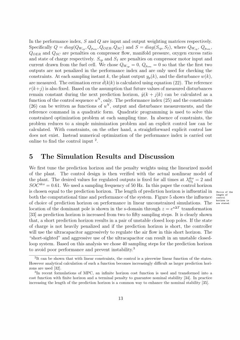
both the computational time and performance of the system. Figure 5 shows the influenceof choice of prediction horizon on performance in linear unconstrained simulations. Thelocation of the dominant pole is shown in the s-domain through z = es∆T transformation[33] as prediction horizon is increased from two to fifty sampling steps. It is clearly shownthat, a short prediction horizon results in a pair of unstable closed loop poles. If the stateof charge is not heavily penalized and if the prediction horizon is short, the controllerwill use the ultracapacitor aggressively to regulate the air flow in this short horizon. The“short-sighted” and aggressive use of the ultracapacitor can result in an unstable closed-loop system. Based on this analysis we chose 40 sampling steps for the prediction horizonto avoid poor performance and prevent instability.3

2It can be shown that with linear constraints, the control is a piecewise linear function of the states.However analytical calculation of such a function becomes increasingly difficult as larger prediction hori-zons are used [32].

3In recent formulations of MPC, an infinite horizon cost function is used and transformed into acost function with finite horizon and a terminal penalty to guarantee nominal stability [34]. In practiceincreasing the length of the prediction horizon is a common way to enhance the nominal stability [35].

13

−15 −10 −5 0 5

−10

−5

0

5

10

10

9

8

7

6

5

4

3

2

1

10

9

8

7

6

5

4

3

2

1

0.9

0.8

0.70.6

0.50.4 0.3 0.2 0.1

0.9

0.8

0.70.6

0.50.4 0.3 0.2 0.1

Real Axis

Imag

inar

y A

xis

S−Domain

unstable region

ω=

ζ=

Incr

easi

ng

Hor

izon

h=30

h=50

h=2

Figure 5: Loci of closed-loop poles in s-domain as prediction horizon increases from h=2 to h=50 steps.The performance index weights are Q = diag(0, 0, 100, 1), S = diag(0.1, 0.001)

10−1

100

101

102

1.9975

1.998

1.9985

1.999

1.9995

2

2.0005

2.001

Min

imum

λO

2

Penalty on State of Discharge (QSC

)

Scp

=0.001S

cp=0.01

Scp

=0.1

10−1

100

101

102

0.4

0.45

0.5

0.55

0.6

0.65

Min

imum

SO

C

Penalty on State of Discharge (QSC

)

10−1

100

101

102

200

300

400

500

600

700

800

Max

imum

Com

pres

sor

Inpu

t (V

olt)

Penalty on State of Discharge (QSC

)

10−1

100

101

102

300

320

340

360

380

400

420

440

Max

imum

FC

Cur

rent

(A

mp)

Penalty on State of Discharge (QSC

)

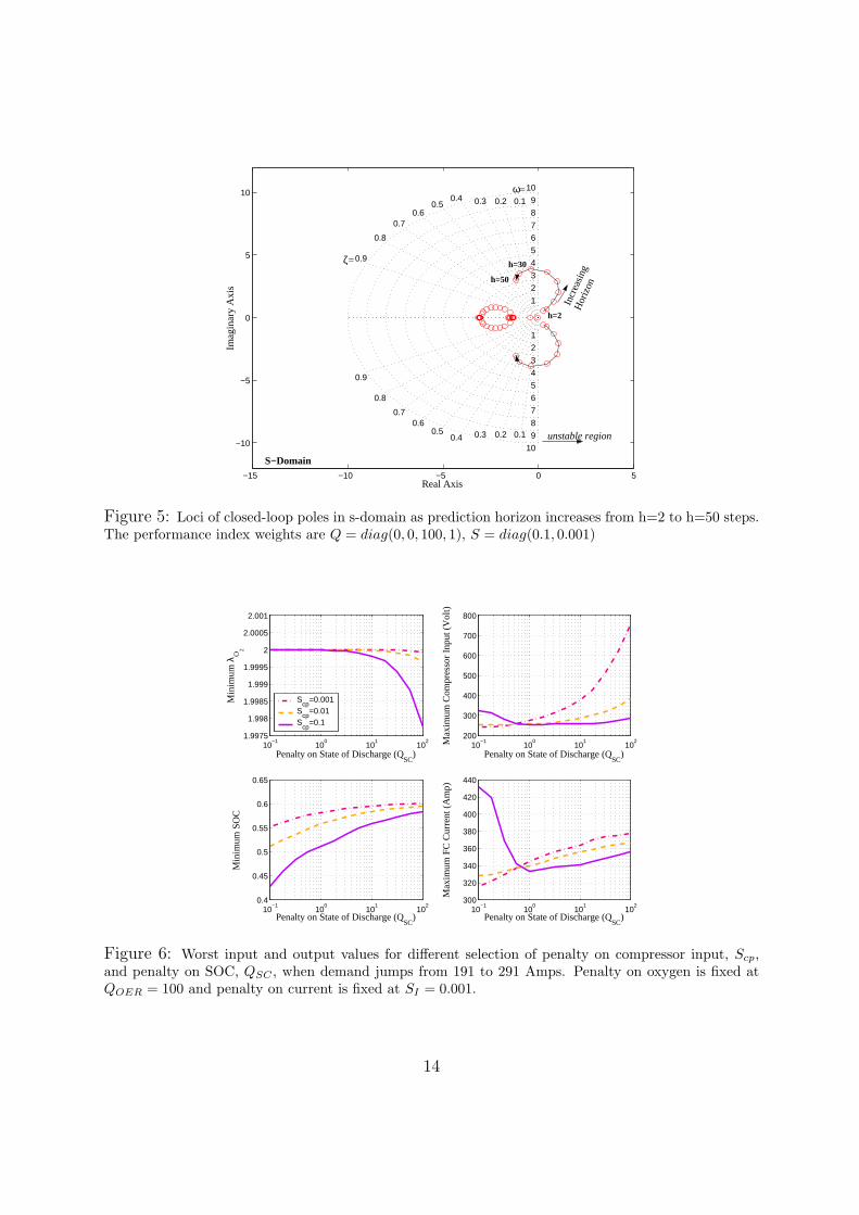
Figure 6: Worst input and output values for different selection of penalty on compressor input, Scp,and penalty on SOC, QSC , when demand jumps from 191 to 291 Amps. Penalty on oxygen is fixed atQOER = 100 and penalty on current is fixed at SI = 0.001.

14

0 0.01 0.02 0.03 0.04 0.05 0.06 0.07 0.08 0.09 0.10.5

1

1.5

2

2.5

3

3.5

4

Compressor Flow (kg/sec)

Pres

sure

Rat

io

Surge Line

Choke Line

ConstrainedUnconstrained

Figure 7: Compressor flow trajectory with and without surge constraint. The performance index weightsare Q = diag(0, 0, 100, 1), S = diag(0.1, 0.001).

The effect of penalty weights on the controller performance is studied next. ConsiderQ = diag(0, 0, QOER, QSC) and S = diag(Scp, SI) in the performance index (25). Theweight on the state of charge, QSC determines the extent to which the ultracapacitor isused. Figure 6 shows the influence of the weights on maximum deviation from nominalvalues of inputs and outputs as the current demand increases from 191 to 291 Amps4. Ineach plot, the x-axis shows the penalty on the state of charge and each curve correspondsto a different penalty on compressor voltage. Penalty on OER is fixed at 100 and penaltyon current is fixed at SI = 0.001. Based on Fig. 6, we chose the penalty on state of chargeto be 1 and the penalty on compressor input at 0.1. These values result in good oxygenregulation with minimum compressor use and maximum utilization of the ultracapacitor(minimum SOC almost equal to 0.5) for 100 Amps increase in current. Therefore for therest of simulations, the penalty matrices Q = diag(0, 0, 100, 1) and S = diag(0.1, 0.001)are fixed.

After a suitable prediction horizon and penalty weights have been chosen, uncon-strained and constrained case are compared through nonlinear simulations. In the con-strained case all the constraints given in equation (26) are active. We simulated thesystem during a sequence of steps in current demand. Figure 7 compares the trajectoryof the compressor flow for the unconstrained and constrained case. Figure 8 shows thecorresponding time history of the response. In both unconstrained and constrained simu-lations, during step changes in the demand, the ultracapacitor is used as a buffer. Duringstep-up in demand, the current that is drawn from the fuel cell and passed through the

4A simple kinetic energy calculation shows that accelerating a 1000 kg vehicle from 20m/s to 21.5m/s(45 mph to 48 mph) in 1 second requires an almost 100 Amps increase in current on a 350 volt BUS.

15

0 2 4 6 8 10 12 14 16 18 201.8

1.9

2

2.1

2.2

λ O2

UnconstrainedConstrained

0 2 4 6 8 10 12 14 16 18 200.5

0.55

0.6

0.65

0.7SO

C

0 2 4 6 8 10 12 14 16 18 20100

150

200

250

Com

pres

sor

Inpu

t(v

olts

)

0 2 4 6 8 10 12 14 16 18 20100

150

200

250

300

Cur

rent

(Am

ps)

Time (seconds)

Idc

UnconstrainedIdc

ConstrainedIdes

SOCmax

=0.66

SOCmin

=0.56

Figure 8: Influence on time response when surge constraint is enforced. The performance index weightsare Q = diag(0, 0, 100, 1), S = diag(0.1, 0.001).

DC/DC convertor, Idc, is initially less than the demand current, Ides, but rises smoothlyto catch up with the demand. As a result oxygen deficit reduces to negligible levels asshown in both simulations. When the fuel cell current tops the demand, the ultracapaci-tor starts to recharge. Enforcing the constraints ensures that the state of charge remainsbetween the specified bounds as shown in Fig. 8. At t = 4 a sudden 40 Amp dip incurrent results in compressor surge in the unconstrained system. In the constrained simu-lation, the current transient and consequently the compressor input transients are sloweddown and as a result surge is prevented. At the same time the excess current charges theultracapacitor as much as the ultracapacitor constraint allows. Once surge is inactive, theenergy stored in the ultracapacitor is released and the state of charge is brought back tothe desired level. A similar response can be seen at t = 12. Note that choke constraint isnot activated even during the large step-up at t = 8.

Simulation also shows that beyond the surge line the compressor behavior is substan-tially different from prediction of the linearized model. This model mismatch causes theoverall closed-loop response of the unconstrained system to degrade as can be seen att = 12. Confining the compressor operation between the surge and choke lines, avoidsregions with large model mismatch and results in improved closed-loop performance. Con-trol of the hybrid fuel cell as explained above reduces the compressor overload that occursduring rapid load transients and might allow use of smaller compressors.

The simulations were performed on a 2 GHz Intel5 Pentium processor on a Windows This

paragraph is

a new

addition

which

discusses the

computation

time required

for solving

the

constrained

versus the

unconstrained

problem.

16

XP 6 operating system. The unconstrained simulation did not require online optimization.Calculating the control gain and running the linear internal model required less than 0.3seconds7 for the 20 second unconstrained simulation shown in Fig. 8. This time doesnot include the runtime for the nonlinear plant since in reality the plant outputs areavailable through measurement and do not require simulation. The constrained simulationrequired solving a quadratic program online. For the 20-second simulation shown inFig. 8, the total CPU time spent on optimization and running the linear internal model(and not including the simulation of the plant) was 20.1 seconds. The CPU time of20.1 seconds for a 20-second constrained simulation is promising, even though we knowthat the state-of-the-art 2.0 GHz processor is considerably faster than the automotivemicrocontroller used in practice. It is also expected that the simulations can be executedmore efficiently in a real-time environment. The feasibility of real-time implementationof a similar optimization-based control method for the same fuel cell system is shown in[36].

6 ConclusionsAn ultracapacitor was utilized to prevent fuel cell oxygen starvation and air compressorsurge during rapid load demands. A model predictive controller was designed for optimaldistribution of current demand between the two power sources. Choice of model predictivecontrol over conventional control methodologies was motivated by the need for smoothcurrent split between the power sources and existence of hard constraints in the auxiliarypower source and the air compressor. The controller performance was verified on a detailednonlinear model of the fuel cell system. The controller performs well in splitting thedemand between the fuel cell and the ultracapacitor. As a result, during a 100 Ampstep-up in current in the hybrid architecture, the oxygen excess ratio always stays above1.98, whereas in the stand alone fuel cell, oxygen excess ratio reaches the critical value of1 as shown in [18]. Model predictive control enforces ultracapacitor constraints on stateof charge and also prevents compressor surge.

7 Appendix

This Appendix provides a summary of fuel cell model governing equations and parameters.Table 1 lists the parameters and variables of the model. The model is explained inmore detail in [19]. Tables 2 and 3 summarize the fuel cell and compressor equations,respectively.

5Intel is a registered trademark of Intel Corporation, Santa Clara, CA.6Windows is a registered trademark of Microsoft Corporation, Seattle, WA.7The cputime command in Matlab was used to get an estimate of the computation time.

17

Table 1: Model Variables and ParametersAfc active area of the fuel cellCD nozzle discharge coefficientDw diffusion coefficientF Farady numberI currentJ compressor inertiaM molar massP powerR universal gas constantT temperatureV volumeW mass flow ratedc compressor diameteri fuel cell current density (I/Afc)m massn number of cellsnd electro-osmotic coefficientp pressuretm membrane thicknessv voltageΩ humidity ratioγ ratio of gas heat capacityφ relative humidityω rotational speedρa air density

Sub/SuperscriptsH2 HydrogenN2 NitrogenO2 Oxygenv vaporw waterin incomingout outgoingrct reactedmbr exchanged through membranepurge purgedan anodeca cathodecm compressor motorcp compressorfc fuel cellrm return manifoldsm supply manifoldst stack

18

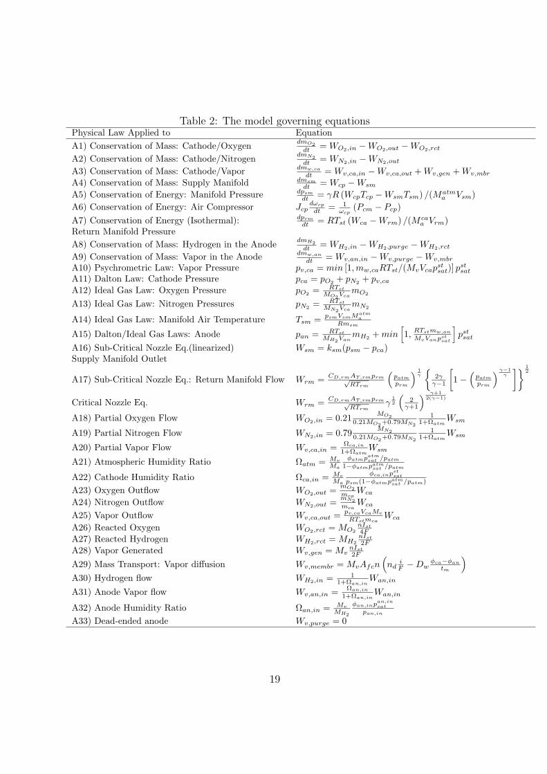
Table 2: The model governing equationsPhysical Law Applied to EquationA1) Conservation of Mass: Cathode/Oxygen dmO2

dt = WO2,in −WO2,out −WO2,rct

A2) Conservation of Mass: Cathode/Nitrogen dmN2dt = WN2,in −WN2,out

A3) Conservation of Mass: Cathode/Vapor dmw,ca

dt = Wv,ca,in −Wv,ca,out + Wv,gen + Wv,mbr

A4) Conservation of Mass: Supply Manifold dmsm

dt = Wcp −Wsm

A5) Conservation of Energy: Manifold Pressure dpsm

dt = γR (WcpTcp −WsmTsm) /(Matma Vsm)

A6) Conservation of Energy: Air Compressor Jcpdωcp

dt = 1ωcp

(Pcm − Pcp)A7) Conservation of Energy (Isothermal): dprm

dt = RTst (Wca −Wrm) /(M caa Vrm)

Return Manifold PressureA8) Conservation of Mass: Hydrogen in the Anode dmH2

dt = WH2,in −WH2,purge −WH2,rct

A9) Conservation of Mass: Vapor in the Anode dmw,an

dt = Wv,an,in −Wv,purge −Wv,mbr

A10) Psychrometric Law: Vapor Pressure pv,ca = min [1,mw,caRTst/(MvVcapstsat)] pst

sat

A11) Dalton Law: Cathode Pressure pca = pO2 + pN2 + pv,ca

A12) Ideal Gas Law: Oxygen Pressure pO2 = RTst

MO2VcamO2

A13) Ideal Gas Law: Nitrogen Pressures pN2 = RTst

MN2VcamN2

A14) Ideal Gas Law: Manifold Air Temperature Tsm = psmVsmMatma

Rmsm

A15) Dalton/Ideal Gas Laws: Anode pan = RTst

MH2VanmH2 + min

[1,

RTstmw,an

MvVanpstsat

]pst

sat

A16) Sub-Critical Nozzle Eq.(linearized) Wsm = ksm(psm − pca)Supply Manifold Outlet

A17) Sub-Critical Nozzle Eq.: Return Manifold Flow Wrm = CD,rmAT,rmprm√RTrm

(patm

prm

) 1γ

2γ

γ−1

[1−

(patm

prm

) γ−1γ

] 12

Critical Nozzle Eq. Wrm = CD,rmAT,rmprm√RTrm

γ12

(2

γ+1

) γ+12(γ−1)

A18) Partial Oxygen Flow WO2,in = 0.21 MO20.21MO2+0.79MN2

11+Ωatm

Wsm

A19) Partial Nitrogen Flow WN2,in = 0.79 MN20.21MO2+0.79MN2

11+Ωatm

Wsm

A20) Partial Vapor Flow Wv,ca,in = Ωca,in

1+ΩatmWsm

A21) Atmospheric Humidity Ratio Ωatm = Mv

Ma

φatmpatmsat /patm

1−φatmpatmsat /patm

A22) Cathode Humidity Ratio Ωca,in = Mv

Ma

φca,inpstsat

psm(1−φatmpatmsat /patm)

A23) Oxygen Outflow WO2,out = mO2mca

Wca

A24) Nitrogen Outflow WN2,out = mN2mca

Wca

A25) Vapor Outflow Wv,ca,out = pv,caVcaMv

RTstmcaWca

A26) Reacted Oxygen WO2,rct = MO2nIst

4F

A27) Reacted Hydrogen WH2,rct = MH2nIst

2F

A28) Vapor Generated Wv,gen = MvnIst

2F

A29) Mass Transport: Vapor diffusion Wv,membr = MvAfcn(nd

iF −Dw

φca−φan

tm

)

A30) Hydrogen flow WH2,in = 11+Ωan,in

Wan,in

A31) Anode Vapor flow Wv,an,in = Ωan,in

1+Ωan,inWan,in

A32) Anode Humidity Ratio Ωan,in = Mv

MH2

φan,inpan,insat

pan,in

A33) Dead-ended anode Wv,purge = 0

19

Table 3: Calculation of Compressor FlowDescription EquationA34)Temperature Correction Factor θ = Tcp,in/(288K)A35)Pressure Correction Factor δ = pcp,in/(1atm)A36)Compressor Speed Correction(rpm) Ncr = Ncp/

√θ

A37)Air Mass Flow Wcp = Wcrδ/√

θA38)Corrected Air mass flow Wcr = Φρa

π4 d2

cUc

A39)Compressor Blade Speed (m/s) Uc = π60dcNcr

A40)Normalized flow rate Φ = Φmax

[1− exp

(β( Ψ

Ψmax− 1)

)]

A41)Dimensionless head parameter Ψ =CpTcp,in

"“pcp,outpcp,in

” γ−1γ −1

#

12 U2

c

A42)Polynomial functions Φmax = a4M4 + a3M

3 + a2M2 + a1M + a0

β = b2M2 + b1M + b0

Ψmax = c5M5 + c4M4 + c3M

3 + c2M2 + c1M + c0

A43)Inlet Mach Number M = Uc√γRaTcp,in

20

8 AcknowledgementsThe authors thank Dr. Ilya Kolmanovsky of Ford Motor Company for his helpful adviceand feedback.

References

[1] R.-H. Song, C.-S. Kim, and D.R. Shin, “Effects of flow rate and starvation of reactant gases on theperformance of phosphoric acid fuel cells,” Journal of Power Sources, vol. 86, pp. 289–293, 2000.

[2] G. Boehm, D. Wilkinson, S. Khight, R. Schamm, and N. Fletcher, “Method and apparatus foroperating a fuel cell,” United States Patents 6,461,741, 2002.

[3] J. Pukrushpan, A. Stefanopoulou, and H. Peng, “Control of fuel cell breathing,” IEEE ControlSystems Magazine, vol. 24, no. 2, pp. 30–46, April 2004.

[4] B. de Jager, “Rotating stall and surge control: a survey,” Proceedings of the 34th Conference onDecision and Control, pp. 1857–1862, December 1995.

[5] P. Moraal and I. Kolmanovsky, “Turbocharger modeling for automotive control applications,” SAEPaper 1999-01-0908, 1999.

[6] D. Boettner, G. Paganelli, Y. Guezennec, G. Rizzoni, and M. Moran, “Proton exchange membranefuel cell system model for automotive vehicle simulation and control,” ASME Journal of EnergyResources Technology, vol. 124, pp. 20–27, 2002.

[7] J. Sun and I. Kolmanovsky, “A robust load governor for fuel cell oxygen starvation protection,”Proceedings of the American Control Conference, pp. 828–833, 2004.

[8] K. Rajashekara, “Propulsion system strategies for fuel cell vehicles,” SAE Paper 2000-01-0369,2000.

[9] N. Jalil, N.A. Kheir, and M. Salman, “A rule-based energy management strategy for a series hybridvehicle,” Proceedings of American Control Conference, pp. 689–693, 1997.

[10] Z. Fillipi, L. Louca, A. Stefanopoulou, J. Pukrushpan, B. Kittirungsi, and H. Peng, “Fuel cell APUfor silent watch and mild electrification of a medium tactical truck,” SAE Paper No 2004-01-1477,2004.

[11] C.-C. Lin, H. Peng, J.-M. Kang, and J. Grizzle, “Power management strategy for a parallel hybridelectric truck,” IEEE Transactions on Control Systems Technology, vol. 11, no. 6, pp. 839–849, 2003.

[12] A. Brahma, Y. Guezennec, and G. Rizzoni, “Optimal energy management in series hybrid electricvehicles,” Proceedings of the American Control Conference, pp. 60–64, 2000.

[13] P. Rodatz, O. Garcia, L. Guzzella, F. Buchi, M. Bartschi, A. Tsukada, P. Dietrich, R. Kotz,G. Scherer, and A. Wokaun, “Performance and operational characteristics of a hybrid vehicle pow-ered by fuel cells and supercapacitors,” SAE Paper 2003-01- 0418, 2003.

[14] T. Matsumoto, N. Watanabe, H. Sugiura, and T. Ishikawa, “Development of fuel-cell hybrid vehicle,”SAE Paper No. 2002-01-0096, 2002.

[15] L.P. Jarvis, P.J. Cygan, and M.P. Roberts, “Hybrid power source for manportable applications,”IEEE AESS Systems Magazine, pp. 13–16, 2003.

[16] Y. Guezennec, T.-Y. Choi, G. Paganelli, and G. Rizzoni, “Supervisory control of fuel cell vehiclesand its link to overall system efficiency and low-level control requirements,” Proceedings of theAmerican Control Conference, pp. 2055–2061, 2003.

21

[17] P. Rodatz, G. Paganelli, A. Sciarretta, and L. Guzzella, “Optimal power management of an experi-mental fuel cell supercapacitor-powered hybrid vehicle,” Control Engineering Practice, vol. 13, pp.41–53, 2005.

[18] A. Vahidi, A. Stefanopoulou, and H. Peng, “Model predictive control for starvation prevention in ahybrid fuel cell system,” Proceedings of American Control Conference, pp. 834–839, 2004.

[19] J. Pukrushpan, A. Stefanopoulou, and H. Peng, Control of Fuel Cell Power Systems: Principles,Modeling, Analysis, and Feedback Design, Springer-Verlag, London, UK, 2004.

[20] J. Pukrushpan, H. Peng, and A. Stefanopoulou, “Control-oriented modeling and analysis for auto-motive fuel cell systems,” ASME Journal of Dynamic Systems, Measurement and Control, vol. 126,pp. 14–25, 2004.

[21] P. Rodatz, G. Paganelli, and L. Guzzella, “Optimizing air supply control of a PEMFC fuel cellsystem,” Proceedings of the American Control Conference, pp. 2043–2048, 2003.

[22] C.-C. Lin, H. Peng, J. Grizzle, and M.J. Kim, “Integrated dynamic simulation model with supervi-sory control strategy for a PEM fuel cell hybrid vehicle,” Proceedings of IMECE 2004 Proceedingsof the ASME Dynamic Systems and Control Division, vol. 73, pp. 275–286, 2004.

[23] J.M. Cunningham, M.A. Hoffman, R.M. Moore, and D.J. Friedman, “Requirements for flexible andrealistic air supply model for incorporation into a fuel cell vehicle (FCV) system simulation,” SAEPaper 1999-01-2912, 1999.

[24] M. Boyce, Gas Turbine Engineering Handbook, Gulf Publishing, Houston, Texas, 1982.

[25] J. Gravdahl and O. Egeland, Compressor Surge and Rotating Stall, Springer, London, UK, 1999.

[26] S. Piller, M. Perrin, and A. Jossen, “Methods for state-of-charge determination and their applica-tions,” Journal of Power Sources, vol. 96, pp. 113–120, 2001.

[27] J.M. Maciejowski, Predictive Control with Constraints, Prentice Hall, Essex, England, 2002.

[28] S. Qin and T. Badgwell, “A survey of industrial model predictive control technology,” ControlEngineering Practice, vol. 11, no. 7, pp. 733–764, July 2003.

[29] D. Mayne, J. Rawlings, C. Rao, and P. Scokaert, “Constrained model predictive control: Stabilityand optimality,” Automatica, vol. 36, pp. 789–814, 2000.

[30] G. Pannocchia and J. Rawlings, “Disturbance models for offset-free model-predictive control,”AIChE Journal, vol. 49, no. 2, pp. 426–437, 2003.

[31] K. Muske and T. Badgwell, “Disturbance modeling for offset-free linear model predictive control,”Journal of Process Control, vol. 12, pp. 617–632, 2002.

[32] P. Tondel, T. Johansen, and A. Bemporad, “An algorithm for multi-parametric quadratic program-ming and explicit MPC solutions,” Automatica, vol. 39, no. 3, pp. 489–497, March 2003.

[33] G. Franklin, D. Powell, and M. Workman, Digital Control of Dynamic Systems, Addison-Wesley,third edition, 1998.

[34] K.R. Muske and J.B. Rawlings, “Model predictive control with linear models,” AIChE Journal, vol.39, no. 2, pp. 262–287, 1993.

[35] D.W. Clarke, Advances in Model-Based Predictive Control, Oxford University Press, 1994.

[36] A. Vahidi, I.V. Kolmanovsky, and A. Stefanopoulou, “Constraint management in fuel cells: A fastreference governor approach,” Proceedings of American Control Conference, pp. 834–839, 2005.

22