JMLR: Workshop and Conference Proceedings 45:269–284, 2015 ACML 2015

Curriculum Learning of Bayesian Network Structures

Yanpeng Zhao1 zhaoyp1@shanghaitech.edu.cn

Yetian Chen2 yetianc@iastate.edu

Kewei Tu1 tukw@shanghaitech.edu.cn

Jin Tian2 jtian@iastate.edu1School of Information Science and Technology, ShanghaiTech University, Shanghai, China2Department of Computer Science, Iowa State University, Ames, IA, USA

Editor: Geoffrey Holmes and Tie-Yan Liu

Abstract

Bayesian networks (BNs) are directed graphical models that have been widely used invarious tasks for probabilistic reasoning and causal modeling. One major challenge inthese tasks is to learn the BN structures from data. In this paper, we propose a novelheuristic algorithm for BN structure learning that takes advantage of the idea of curriculumlearning. Our algorithm learns the BN structure by stages. At each stage a subnet islearned over a selected subset of the random variables conditioned on fixed values of therest of the variables. The selected subset grows with stages and eventually includes all thevariables. We prove theoretical advantages of our algorithm and also empirically show thatit outperformed the state-of-the-art heuristic approach in learning BN structures.

Keywords: Bayesian networks, structure learning, curriculum learning.

1. Introduction

A Bayesian network (BN) is a directed acyclic graph (DAG) where nodes are randomvariables and directed edges represent probability dependencies among variables. Eachnode and its parents are associated with a conditional probability distribution (CPD), whichquantifies the effect of the parents on the node. A BN provides a compact representation of ajoint probability distribution over the set of random variables. These models are also calledbelief networks, or causal networks, because the directed edges are sometimes interpretedas causal relations. BNs have been widely used in various tasks for probabilistic inferenceand causal modeling (Pearl, 2000; Spirtes et al., 2001). A major challenge in these tasks isto learn the structure and the associated CPDs from data.

Learning a BN is usually conducted in two phases. In the first phase, one manages toconstruct the topology (structure) of the network. In the second phase, one then estimatesthe parameters of the CPDs given the fixed structure. Parameter estimation in the secondphase is considered a well-studied problem. The learning of the topology, or in other words,structure learning, is more challenging.

1.1. Previous Work on Bayesian Network Structure Learning

There has been an enormous amount of work on learning BNs from data. Methods for thislearning problem fall into two categories: constraint-based and score-based.

c© 2015 Y. Zhao, Y. Chen, K. Tu & J. Tian.

Zhao Chen Tu Tian

Constraint-based algorithms look for conditional independencies (CIs) in the data andbuild the DAG consistent to these CIs. Well-known examples are the Peter-Clark (PC)algorithm (Spirtes et al., 2001) and the Inductive-Causation (IC) algorithm (Pearl, 2000).Other later work includes the Grow-Shrink (GS) and Total-Conditioning (TC) algorithms(Margaritis and Thrun, 2000; Pellet and Elisseeff, 2008). PC or IC algorithms are guar-anteed to return a DAG that exactly represents the CI relationships implied by the targetdistribution if all CI tests are perfect. Such assumption certainly does not hold in realitysince any kind of statistical test will have some probability of making errors given limiteddata samples. Even worse, an error of a statistical test can result in propagated errors inthe subsequent learning process.

Score-based approaches convert the problem to an optimization problem, where a de-composable score is used to measure the fitness of a DAG to the observed data, then asearch strategy is employed to maximize (or minimize) the score over the space of pos-sible DAGs (Cooper and Herskovits, 1992; Heckerman et al., 1995). However, finding anoptimal BN structure is NP-hard (Chickering, 1996). Algorithms in this category includeexact algorithms that are able to find an optimal solution or heuristic algorithms that of-ten return sub-optimal models. The research on exact algorithms started with a familyof algorithms using dynamic programming (DP) (Koivisto and Sood, 2004; Silander andMyllymaki, 2006). These DP algorithms require exponential time and space, thus are onlyapplicable to problems with up to 30 variables. Latest work in this area used A* or othertechniques to prune the search space so that both time and space complexities were greatlyreduced (Yuan et al., 2011; Malone et al., 2011; Yuan and Malone, 2012). Recently, a set ofalgorithms using Integer Linear Programming (ILP) are showed being competitive with theA* algorithm (Jaakkola et al., 2010; Bartlett and Cussens, 2013). In particular, GOBNILP(Globally Optimal BN learning using ILP) was demonstrated to be able to handle problemswith up to a few hundred variables (Bartlett and Cussens, 2013). However, it assumes theindegree of each node is upper-bounded by a small constant.

Heuristic search method encompasses a broad class of algorithms, varying in the scoringfunctions being used, the search strategies being employed, and assumptions being made.The general search strategy is, given a starting point, i.e., any DAG, by adding, deleting orreversing one or a few edges, the algorithm manages to traverse the DAG space to find ahigh-scoring model. However, there are super-exponential number of possible DAGs. Thus,local search strategies such as greedy or more sophisticated search algorithms are oftenused. The searches will often stuck in local maxima.

Finally, ideas combining both constraint-based and score-based approaches have alsobeen explored. A well-known algorithm is Max-Min Hill-Climbing (MMHC) algorithm(Tsamardinos et al., 2006). MMHC first estimates the parents and children (PC ) set ofeach variable using a local discovery algorithm called MMPC (Tsamardinos et al., 2003).It then performs a Bayesian-scoring greedy hill-climbing search with the constraint that theneighbors of each variable must be in the variable’s PC set. Extensive empirical evaluationshowed that MMHC outperformed on average other heuristic algorithms thus it was claimedto be the current state-of-the-art. MMHC is a two-stage algorithm. In the first stage, theidentification of the PC sets involves a large number of CI tests, which are very sensitiveto noises in data. Thus, the problem of constraint-based method may also trap MMHC.

270

Curriculum Learning of Bayesian Network Structures

An empirical evaluation of the impact of learning strategies on the quality of BNs canbe found in (Malone et al., 2015).

1.2. Curriculum Learning

Humans and animals learn much better when the examples are not randomly presented butorganized in a meaningful order which starts from relatively simple concepts and graduallyintroduces more complex ones. This idea has been formalized in the context of machinelearning as curriculum learning (Bengio et al., 2009). A curriculum is a sequence of weight-ing schemes of the training data, denoted by (W1,W2, ...,Wm). The first scheme W1 assignsmore weight to “easier” training samples, and each next scheme assigns slightly more weightto “harder” examples, until the last scheme Wm that assigns uniform weight to all exam-ples. Ideally, the information entropy of the weighting scheme shall increase monotonically,i.e., ∀i < j, H(Wi) < H(Wj). How to measure the “easiness” or complexity of trainingsamples may vary depending on the learning problems, and no general measurement hasbeen proposed. Learning is done iteratively, each time from the training data weightedby the current weighting scheme and initialized with the learning result from the previousiteration.

Curriculum learning has been successfully applied to many problems, such as learninglanguage models and grammars (Elman, 1993; Spitkovsky et al., 2010; Tu and Honavar,2011) and object recognition and localization (Kumar et al., 2010). There have also beenattempts to explain the advantages of curriculum learning. Bengio et al. (2009) proposedthat a well chosen curriculum strategy can act as a continuation method (Allgower andGeorg, 1990), which first optimizes a highly smoothed objective and then gradually considersless smoothing. Tu and Honavar (2011) contended that in learning structures such asgrammars, an ideal curriculum decomposes the structure into multiple components andguides the learner to incrementally construct the target structure. More recently, a fewextensions of the original idea of curriculum learning have been proposed (Kumar et al.,2010; Jiang et al., 2015).

In BN structure learning, one needs to discover the conditional independence/dependencebetween variables. Most of the current approaches try to learn these relations between allthe variables by looking at all the training samples at once. In contrast, human rarelylook at all the variables and samples at once during learning; instead, they learn in a moreorganized way, starting with more common data samples that involve dependency relationsbetween only a small subset of variables (typically with the other variables fixed at certainvalues), and only turning to less common data samples involving dependency relations withadditional variables when some knowledge (i.e., a partial model) is obtained. In this way,learning could be made more accurate and even more efficient. This learning strategy canbe seen as a type of curriculum learning, related to the idea of incremental construction (Tuand Honavar, 2011) mentioned above. In this paper, we design a novel heuristic algorithmfor BN structure learning that takes advantage of this idea. Our algorithm learns the BNstructure by stages. At each stage a subnet is learned over a selected subset of the randomvariables conditioned on fixed values of the rest of the variables. The selected subset growswith stages until it includes all the variables at the final stage. Figure 1 shows an illustra-tive example of our algorithm. We prove theoretical advantages of our algorithm and also

271

Zhao Chen Tu TianAS TLB E XDvariable sequence �

0 1 2 3 4 5 6 7

A S

T L B

E

X D

A S

T L B

E

X D

A S

T L B

E

X D

A S

T L B

E

X D

G1 G2 G3

Figure 1: An illustrative example of curriculum learning of a BN structure. Given a curriculum({S,B,D}, {S,B,D,L,E,X}, {S,B,D,L,E,X,A, T}) and step size t = 3, we learn theBN structure in three stages: (1) learn a subnet G1 over {S,B,D} from scratch; (2) learna larger subnet G2 over {S,B,D,L,E,X} with G1 as the start point of search; (3) learna full network with G2 as the start point. Each subnet (in red) is conditioned on the restof the variables (in green).

empirically show that it outperformed the state-of-the-art heuristic approach in learningBN structures.

2. Preliminaries

Formally, a Bayesian network is a pair B = (G,P ), where G is a DAG that encodes ajoint probability distribution P over a vector of random variables X = (X1, ..., Xn) witheach node of the graph representing a variable in X. For convenience we typically work onthe index set V = {1, ..., n} and represent a variable Xi by its index i. The DAG can berepresented as a vector G = (Pa1, ..., Pan) where each Pai is a subset of the index set Vand specifies the parents of i in the graph.

Definition 1 (I-equivalence) (Verma and Pearl, 1990) Two DAG G1 and G2 over thesame set of variables X are I-equivalent if they represent the same set of conditional inde-pendence relations.

Two I-equivalent DAGs are statistically indistinguishable. That is, given observational data,it is impossible to identify a unique data-generating DAG unless there is only one DAG inthe corresponding equivalence class (EC). All BNs in an EC have the same skeleton andthe same v-structures1 (Verma and Pearl, 1990). Thus, we can represent an EC using acomplete partially DAG (CPDAG) which consist of a directed edge for every irreversibleedge and an undirected edge for every reversible edge.2

In the problem of learning BNs from data, we assume that a complete data D aregenerated i.i.d from an underlying distribution P ∗(X) which is induced by some BN B∗ =(G∗, P ∗). Due to the so called I-equivalence, the best we can hope is to recover G∗’sequivalence class. That is, we target any G that is I-equivalent to G∗.

In this paper, we focus on score-based search. The first component of the score-and-search method is a scoring criterion measuring the fitness of a DAG G to the data D.Several commonly used scoring functions are MDL, AIC, BIC and Bayesian score. In this

1. A v-structure in a DAG G is an ordered triple of nodes (u, v, w) such that G contains the directed edgesu → v and w → v and u and w are not adjacent in G.

2. A CPDAG is also called a pattern. Each equivalence class has a unique CPDAG.

272

Curriculum Learning of Bayesian Network Structures

work, we use Bayesian score, defined as follows.

score(G : D) = logP (D|G) + logP (G), (1)

where P (D|G) is the likelihood of the data given the DAG G and P (G) is the prior over theDAG structures. In this work, we assume discrete random variables which follow a Dirichlet-Multinomial distribution. That is, each variable Xi follows a multinomial distribution withparameter vector Θi conditioning on its parents, and the parameter vector Θi follows aDirichlet distribution with parameter vector αi as the prior. Assuming global and localparameter independence, parameter modularity, and uniform structure prior P (G), thescore is decomposable (Heckerman et al., 1995):

score(G : D) =n∑

i=1

scorei(Pai : D), (2)

where scorei(Pai : D) is called the local score or family score measuring how well a set ofvariables Pai serves as parents of Xi. scorei(Pai : D) can be computed efficiently from thesufficient statistics of the data D. Further we can show for any two I-equivalent DAGs G1

and G2, score(G1 : D) = score(G2 : D). This is called score equivalence. The commonlyused scoring functions such as MDL, AIC, BIC and BDe all satisfy score decomposabilityand equivalence.

3. Curriculum Learning of Bayesian Network Structures

The basic idea to apply curriculum learning and incremental construction in BN structurelearning is that we can define a sequence of intermediate learning targets (G1, ..., Gm), whereeach Gi is a subnet of the target BN over a subset of variables X(i) conditioned on certainfixed values x′(i) of the rest of the variables X′(i), where X(i) ⊆ X, X′(i) = X \ X(i) andX(i) ⊂ X(i+1); at stage i of curriculum learning, we try to learn Gi from a subset of datasamples with X′(i) = x′(i). In terms of the sample weighting scheme (W1,W2, ...,Wm), each

Wi assigns 1 to those samples with X′(i) = x′(i) and 0 to the other samples.However, training samples are often very limited in practice and thus the subset of sam-

ples with X′(i) = x′(i) would typically be very small. Learning from such small-sized training

sample is deemed unreliable. A key observation is that when we fix X′(i) to different values,our learning target is actually the same DAG structure Gi but with different parameters(CPDs). Thus, we can make use of all the training samples in learning Gi at each stageby revising the scoring function to take into account multiple versions of parameters. Thisstrategy extends the original curriculum learning framework.

Note that in the ideal case, the subnet learned in each stage would have only one type ofdiscrepancy from the truth BN: it would contain extra edges between variables in X(i) dueto conditioning on X′(i). More specifically, such variables in X(i) must share a child node

that is in, or has a descendant in, X′(i) such that they are not d -separated when conditioning

on X′(i).

273

Zhao Chen Tu Tian

3.1. Scoring Function

In this paper, we use Bayesian score to design a scoring function that uses all trainingsamples. Assume the domain for X′(i) is {x′(i),1, ...,x

′(i),q}. Then we can have a set of data

segments Di = {Di,1, ..., Di,q} by grouping samples based on the values of X′(i) and thenprojecting on X(i). Assuming Di,1, ..., Di,q are generated by the same DAG Gi but with“independent” CPDs, we can derive

P (Gi, Di) = P (Gi)

q∏j=1

P (Di,j |Gi) = P (Gi)1−q

q∏j=1

P (Gi, Di,j). (3)

If we take logarithm for both sides, we obtain

logP (Gi, Di) = (1− q) logP (Gi) +

q∑j=1

logP (Gi, Di,j). (4)

If we set uniform prior for Gi, i.e., P (Gi) ∝ 1, we then have

logP (Gi, Di) = C +

q∑j=1

logP (Gi, Di,j), (5)

where C is a constant. We use BDe score (Heckerman et al., 1995) for discrete variables,i.e., logP (Gi, Di,j) = scoreBDe(Gi, Di,j), so we have the following scoring function

score(Gi, Di) =

q∑j=1

scoreBDe(Gi, Di,j), (6)

i.e., the sum of BDe scores which are individually evaluated on each of the data segmentsDi,1, ..., Di,q.

One common problem with curriculum learning is that the learner may overfit theintermediate learning targets, especially when the number of variables is large and thus wehave to divide learning into many stages. Overfitting also occurs when the sample size issmall. Therefore, we introduce a penalty function that penalizes the size of the networkespecially when the number of variables is large or the sample size is small:

Penalty(Gi : Di) =

(a

SS+V (Gi)

b

)E(Gi), (7)

where SS is the sample size, V (Gi) and E(Gi) denote the number of variables and numberof edges in Gi respectively, and a and b are positive constants. Combined with the penaltyfunction, the scoring function becomes

score(Gi : Di) =

q∑j=1

scoreBDe(Gi, Di,j)−(a

SS+V (Gi)

b

)E(Gi). (8)

274

Curriculum Learning of Bayesian Network Structures

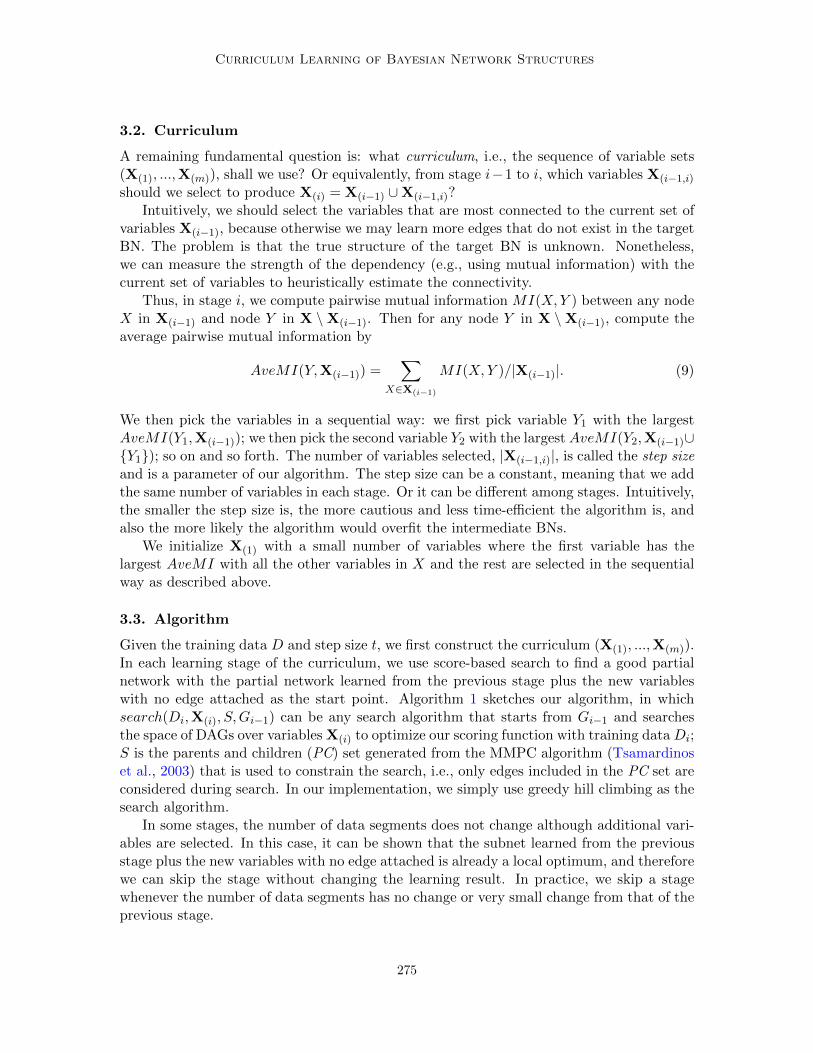
3.2. Curriculum

A remaining fundamental question is: what curriculum, i.e., the sequence of variable sets(X(1), ...,X(m)), shall we use? Or equivalently, from stage i−1 to i, which variables X(i−1,i)should we select to produce X(i) = X(i−1) ∪X(i−1,i)?

Intuitively, we should select the variables that are most connected to the current set ofvariables X(i−1), because otherwise we may learn more edges that do not exist in the targetBN. The problem is that the true structure of the target BN is unknown. Nonetheless,we can measure the strength of the dependency (e.g., using mutual information) with thecurrent set of variables to heuristically estimate the connectivity.

Thus, in stage i, we compute pairwise mutual information MI(X,Y ) between any nodeX in X(i−1) and node Y in X \X(i−1). Then for any node Y in X \X(i−1), compute theaverage pairwise mutual information by

AveMI(Y,X(i−1)) =∑

X∈X(i−1)

MI(X,Y )/|X(i−1)|. (9)

We then pick the variables in a sequential way: we first pick variable Y1 with the largestAveMI(Y1,X(i−1)); we then pick the second variable Y2 with the largest AveMI(Y2,X(i−1)∪{Y1}); so on and so forth. The number of variables selected, |X(i−1,i)|, is called the step sizeand is a parameter of our algorithm. The step size can be a constant, meaning that we addthe same number of variables in each stage. Or it can be different among stages. Intuitively,the smaller the step size is, the more cautious and less time-efficient the algorithm is, andalso the more likely the algorithm would overfit the intermediate BNs.

We initialize X(1) with a small number of variables where the first variable has thelargest AveMI with all the other variables in X and the rest are selected in the sequentialway as described above.

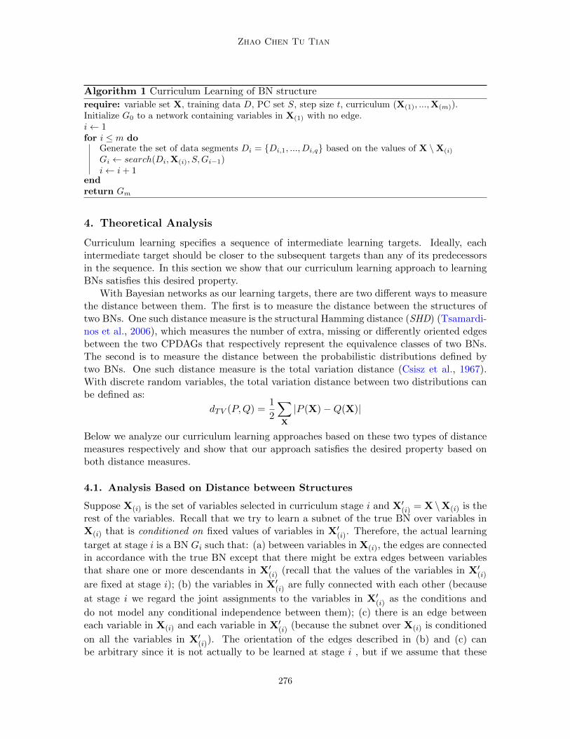
3.3. Algorithm

Given the training data D and step size t, we first construct the curriculum (X(1), ...,X(m)).In each learning stage of the curriculum, we use score-based search to find a good partialnetwork with the partial network learned from the previous stage plus the new variableswith no edge attached as the start point. Algorithm 1 sketches our algorithm, in whichsearch(Di,X(i), S,Gi−1) can be any search algorithm that starts from Gi−1 and searchesthe space of DAGs over variables X(i) to optimize our scoring function with training data Di;S is the parents and children (PC) set generated from the MMPC algorithm (Tsamardinoset al., 2003) that is used to constrain the search, i.e., only edges included in the PC set areconsidered during search. In our implementation, we simply use greedy hill climbing as thesearch algorithm.

In some stages, the number of data segments does not change although additional vari-ables are selected. In this case, it can be shown that the subnet learned from the previousstage plus the new variables with no edge attached is already a local optimum, and thereforewe can skip the stage without changing the learning result. In practice, we skip a stagewhenever the number of data segments has no change or very small change from that of theprevious stage.

275

Zhao Chen Tu Tian

Algorithm 1 Curriculum Learning of BN structure

require: variable set X, training data D, PC set S, step size t, curriculum (X(1), ...,X(m)).Initialize G0 to a network containing variables in X(1) with no edge.i← 1for i ≤ m do

Generate the set of data segments Di = {Di,1, ..., Di,q} based on the values of X \X(i)

Gi ← search(Di,X(i), S,Gi−1)i← i+ 1

endreturn Gm

4. Theoretical Analysis

Curriculum learning specifies a sequence of intermediate learning targets. Ideally, eachintermediate target should be closer to the subsequent targets than any of its predecessorsin the sequence. In this section we show that our curriculum learning approach to learningBNs satisfies this desired property.

With Bayesian networks as our learning targets, there are two different ways to measurethe distance between them. The first is to measure the distance between the structures oftwo BNs. One such distance measure is the structural Hamming distance (SHD) (Tsamardi-nos et al., 2006), which measures the number of extra, missing or differently oriented edgesbetween the two CPDAGs that respectively represent the equivalence classes of two BNs.The second is to measure the distance between the probabilistic distributions defined bytwo BNs. One such distance measure is the total variation distance (Csisz et al., 1967).With discrete random variables, the total variation distance between two distributions canbe defined as:

dTV (P,Q) =1

2

∑X

|P (X)−Q(X)|

Below we analyze our curriculum learning approaches based on these two types of distancemeasures respectively and show that our approach satisfies the desired property based onboth distance measures.

4.1. Analysis Based on Distance between Structures

Suppose X(i) is the set of variables selected in curriculum stage i and X′(i) = X \X(i) is therest of the variables. Recall that we try to learn a subnet of the true BN over variables inX(i) that is conditioned on fixed values of variables in X′(i). Therefore, the actual learning

target at stage i is a BN Gi such that: (a) between variables in X(i), the edges are connectedin accordance with the true BN except that there might be extra edges between variablesthat share one or more descendants in X′(i) (recall that the values of the variables in X′(i)are fixed at stage i); (b) the variables in X′(i) are fully connected with each other (because

at stage i we regard the joint assignments to the variables in X′(i) as the conditions and

do not model any conditional independence between them); (c) there is an edge betweeneach variable in X(i) and each variable in X′(i) (because the subnet over X(i) is conditioned

on all the variables in X′(i)). The orientation of the edges described in (b) and (c) canbe arbitrary since it is not actually to be learned at stage i , but if we assume that these

276

Curriculum Learning of Bayesian Network Structures

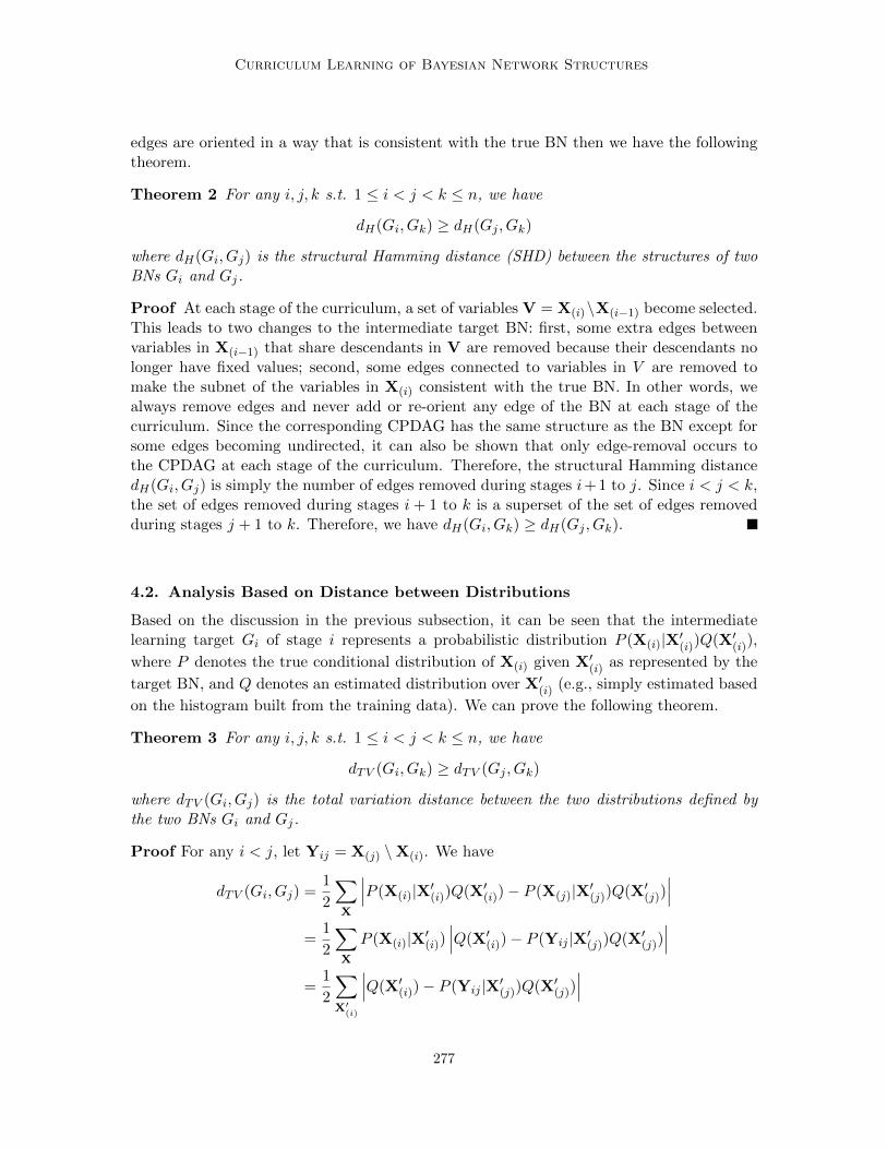
edges are oriented in a way that is consistent with the true BN then we have the followingtheorem.

Theorem 2 For any i, j, k s.t. 1 ≤ i < j < k ≤ n, we have

dH(Gi, Gk) ≥ dH(Gj , Gk)

where dH(Gi, Gj) is the structural Hamming distance (SHD) between the structures of twoBNs Gi and Gj.

Proof At each stage of the curriculum, a set of variables V = X(i)\X(i−1) become selected.This leads to two changes to the intermediate target BN: first, some extra edges betweenvariables in X(i−1) that share descendants in V are removed because their descendants nolonger have fixed values; second, some edges connected to variables in V are removed tomake the subnet of the variables in X(i) consistent with the true BN. In other words, wealways remove edges and never add or re-orient any edge of the BN at each stage of thecurriculum. Since the corresponding CPDAG has the same structure as the BN except forsome edges becoming undirected, it can also be shown that only edge-removal occurs tothe CPDAG at each stage of the curriculum. Therefore, the structural Hamming distancedH(Gi, Gj) is simply the number of edges removed during stages i+ 1 to j. Since i < j < k,the set of edges removed during stages i+ 1 to k is a superset of the set of edges removedduring stages j + 1 to k. Therefore, we have dH(Gi, Gk) ≥ dH(Gj , Gk).

4.2. Analysis Based on Distance between Distributions

Based on the discussion in the previous subsection, it can be seen that the intermediatelearning target Gi of stage i represents a probabilistic distribution P (X(i)|X′(i))Q(X′(i)),

where P denotes the true conditional distribution of X(i) given X′(i) as represented by the

target BN, and Q denotes an estimated distribution over X′(i) (e.g., simply estimated based

on the histogram built from the training data). We can prove the following theorem.

Theorem 3 For any i, j, k s.t. 1 ≤ i < j < k ≤ n, we have

dTV (Gi, Gk) ≥ dTV (Gj , Gk)

where dTV (Gi, Gj) is the total variation distance between the two distributions defined bythe two BNs Gi and Gj.

Proof For any i < j, let Yij = X(j) \X(i). We have

dTV (Gi, Gj) =1

2

∑X

∣∣∣P (X(i)|X′(i))Q(X′(i))− P (X(j)|X′(j))Q(X′(j))∣∣∣

=1

2

∑X

P (X(i)|X′(i))∣∣∣Q(X′(i))− P (Yij |X′(j))Q(X′(j))

∣∣∣=

1

2

∑X′

(i)

∣∣∣Q(X′(i))− P (Yij |X′(j))Q(X′(j))∣∣∣

277

Zhao Chen Tu Tian

Therefore, we have

dTV (Gi, Gk) =1

2

∑X′

(j)

∑Yij

∣∣∣Q(X′(i))− P (Yik|X′(k))Q(X′(k))∣∣∣

and

dTV (Gj , Gk) =1

2

∑X′

(j)

∣∣∣Q(X′(j))− P (Yjk|X′(k))Q(X′(k))∣∣∣

=1

2

∑X′

(j)

∣∣∣∣∣∣∑Yij

Q(X′(i))−∑Yij

P (Yik|X′(k))Q(X′(k))

∣∣∣∣∣∣Because the absolute value is subadditive, we have

∑Yij

∣∣∣Q(X′(i))− P (Yik|X′(k))Q(X′(k))∣∣∣ ≥

∣∣∣∣∣∣∑Yij

(Q(X′(i))− P (Yik|X′(k))Q(X′(k))

)∣∣∣∣∣∣Therefore,

dTV (Gi, Gk) ≥ dTV (Gj , Gk)

5. Experiments

In this section, we empirically evaluate our algorithm and compare it with MMHC (Tsamardi-nos et al., 2006), the current state-of-the-art heuristic algorithm in BN structure learning.For both algorithms, we used BDeu score (Heckerman et al., 1995) with the equivalent sam-ple size 10 as the scoring function and used the MMPC module included in Causal Explorer(Aliferis et al., 2003) with the default setting to generate the PC set. For MMHC, we usedthe settings mentioned by Tsamardinos et al. (2006).

We collected 10 benchmark BNs from the bnlearn repository3. The statistics of theseBNs are shown in Table 1. From each of these BNs, we generated datasets of varioussample sizes (SS = 100, 500, 1000, 5000, 10000, 50000). For each sample size, we randomlygenerated 5 datasets and reported the algorithm performance averaged over these 5 datasets.

When running our algorithm on each dataset, we set the step size (introduced in section3.2) to 1, 2 and 3 and learned three BNs; we also learned a BN by hill climbing with nocurriculum. We then picked the BN with the largest BDeu score as the final output. In ourexperiments, we find that only on a small fraction (50 out of 300) of the datasets did hillclimbing with no curriculum produce the final output. More detailed statistics regarding theeffect of step size on final output can be found in Table S1 of the supplemental material. Wetuned the parameter a and b of the penalty function (Equation 7) on a separate validationset and fixed them to 1000 and 100 respectively.

3. http://www.bnlearn.com/bnrepository/

278

Curriculum Learning of Bayesian Network Structures

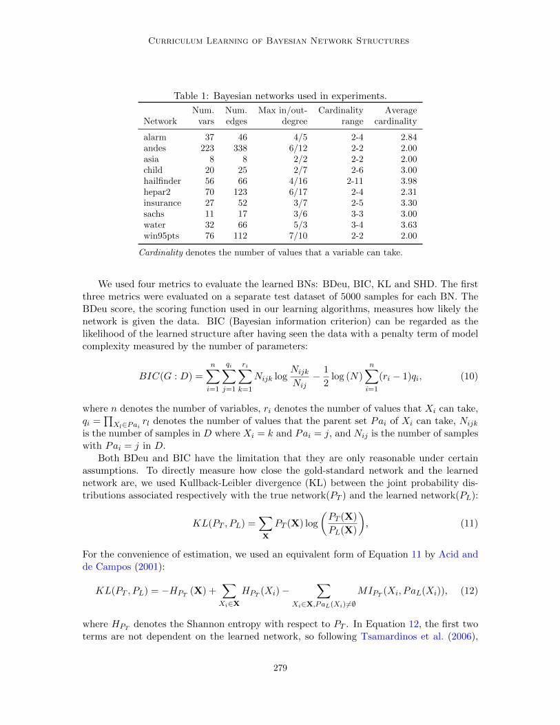
Table 1: Bayesian networks used in experiments.

Num. Num. Max in/out- Cardinality AverageNetwork vars edges degree range cardinality

alarm 37 46 4/5 2-4 2.84andes 223 338 6/12 2-2 2.00asia 8 8 2/2 2-2 2.00child 20 25 2/7 2-6 3.00hailfinder 56 66 4/16 2-11 3.98hepar2 70 123 6/17 2-4 2.31insurance 27 52 3/7 2-5 3.30sachs 11 17 3/6 3-3 3.00water 32 66 5/3 3-4 3.63win95pts 76 112 7/10 2-2 2.00

Cardinality denotes the number of values that a variable can take.

We used four metrics to evaluate the learned BNs: BDeu, BIC, KL and SHD. The firstthree metrics were evaluated on a separate test dataset of 5000 samples for each BN. TheBDeu score, the scoring function used in our learning algorithms, measures how likely thenetwork is given the data. BIC (Bayesian information criterion) can be regarded as thelikelihood of the learned structure after having seen the data with a penalty term of modelcomplexity measured by the number of parameters:

BIC(G : D) =n∑

i=1

qi∑j=1

ri∑k=1

Nijk logNijk

Nij− 1

2log (N)

n∑i=1

(ri − 1)qi, (10)

where n denotes the number of variables, ri denotes the number of values that Xi can take,qi =

∏Xl∈Pai

rl denotes the number of values that the parent set Pai of Xi can take, Nijk

is the number of samples in D where Xi = k and Pai = j, and Nij is the number of sampleswith Pai = j in D.

Both BDeu and BIC have the limitation that they are only reasonable under certainassumptions. To directly measure how close the gold-standard network and the learnednetwork are, we used Kullback-Leibler divergence (KL) between the joint probability dis-tributions associated respectively with the true network(PT ) and the learned network(PL):

KL(PT , PL) =∑X

PT (X) log

(PT (X)

PL(X)

), (11)

For the convenience of estimation, we used an equivalent form of Equation 11 by Acid andde Campos (2001):

KL(PT , PL) = −HPT(X) +

∑Xi∈X

HPT(Xi)−

∑Xi∈X,PaL(Xi)6=∅

MIPT(Xi, PaL(Xi)), (12)

where HPTdenotes the Shannon entropy with respect to PT . In Equation 12, the first two

terms are not dependent on the learned network, so following Tsamardinos et al. (2006),

279

Zhao Chen Tu Tian

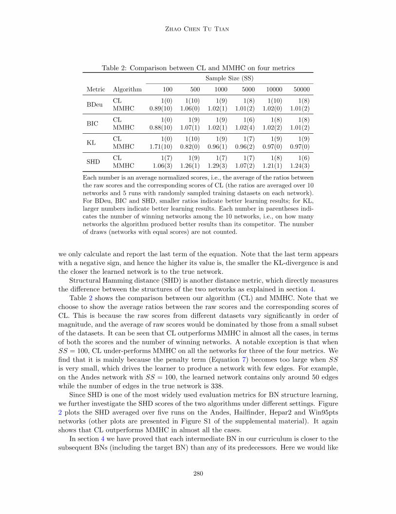
Table 2: Comparison between CL and MMHC on four metrics

Sample Size (SS)

Metric Algorithm 100 500 1000 5000 10000 50000

BDeuCL 1(0) 1(10) 1(9) 1(8) 1(10) 1(8)MMHC 0.89(10) 1.06(0) 1.02(1) 1.01(2) 1.02(0) 1.01(2)

BICCL 1(0) 1(9) 1(9) 1(6) 1(8) 1(8)MMHC 0.88(10) 1.07(1) 1.02(1) 1.02(4) 1.02(2) 1.01(2)

KLCL 1(0) 1(10) 1(9) 1(7) 1(9) 1(9)MMHC 1.71(10) 0.82(0) 0.96(1) 0.96(2) 0.97(0) 0.97(0)

SHDCL 1(7) 1(9) 1(7) 1(7) 1(8) 1(6)MMHC 1.06(3) 1.26(1) 1.29(3) 1.07(2) 1.21(1) 1.24(3)

Each number is an average normalized scores, i.e., the average of the ratios betweenthe raw scores and the corresponding scores of CL (the ratios are averaged over 10networks and 5 runs with randomly sampled training datasets on each network).For BDeu, BIC and SHD, smaller ratios indicate better learning results; for KL,larger numbers indicate better learning results. Each number in parentheses indi-cates the number of winning networks among the 10 networks, i.e., on how manynetworks the algorithm produced better results than its competitor. The numberof draws (networks with equal scores) are not counted.

we only calculate and report the last term of the equation. Note that the last term appearswith a negative sign, and hence the higher its value is, the smaller the KL-divergence is andthe closer the learned network is to the true network.

Structural Hamming distance (SHD) is another distance metric, which directly measuresthe difference between the structures of the two networks as explained in section 4.

Table 2 shows the comparison between our algorithm (CL) and MMHC. Note that wechoose to show the average ratios between the raw scores and the corresponding scores ofCL. This is because the raw scores from different datasets vary significantly in order ofmagnitude, and the average of raw scores would be dominated by those from a small subsetof the datasets. It can be seen that CL outperforms MMHC in almost all the cases, in termsof both the scores and the number of winning networks. A notable exception is that whenSS = 100, CL under-performs MMHC on all the networks for three of the four metrics. Wefind that it is mainly because the penalty term (Equation 7) becomes too large when SSis very small, which drives the learner to produce a network with few edges. For example,on the Andes network with SS = 100, the learned network contains only around 50 edgeswhile the number of edges in the true network is 338.

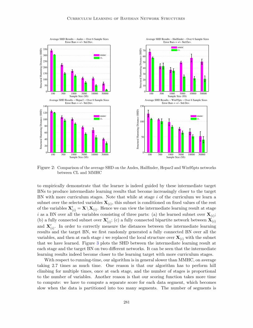
Since SHD is one of the most widely used evaluation metrics for BN structure learning,we further investigate the SHD scores of the two algorithms under different settings. Figure2 plots the SHD averaged over five runs on the Andes, Hailfinder, Hepar2 and Win95ptsnetworks (other plots are presented in Figure S1 of the supplemental material). It againshows that CL outperforms MMHC in almost all the cases.

In section 4 we have proved that each intermediate BN in our curriculum is closer to thesubsequent BNs (including the target BN) than any of its predecessors. Here we would like

280

Curriculum Learning of Bayesian Network Structures

100 500 1000 5000 10000 500000

50

100

150

200

250

300

350

Sample Size (SS)

Str

uct

ura

l H

amm

ing D

ista

nce

(S

HD

)Average SHD Results − Andes − Over 6 Sample Sizes

Error Bars = +/− Std.Dev.

MMHC

CL

100 500 1000 5000 10000 500000

10

20

30

40

50

60

70

Sample Size (SS)

Str

uct

ura

l H

amm

ing D

ista

nce

(S

HD

)

Average SHD Results − Hailfinder − Over 6 Sample SizesError Bars = +/− Std.Dev.

MMHC

CL

100 500 1000 5000 10000 500000

20

40

60

80

100

120

140

Sample Size (SS)

Str

uct

ura

l H

amm

ing D

ista

nce

(S

HD

)

Average SHD Results − Hepar2 − Over 6 Sample SizesError Bars = +/− Std.Dev.

MMHC

CL

100 500 1000 5000 10000 500000

50

100

150

Sample Size (SS)

Str

uct

ura

l H

amm

ing D

ista

nce

(S

HD

)

Average SHD Results − Win95pts − Over 6 Sample SizesError Bars = +/− Std.Dev.

MMHC

CL

Figure 2: Comparison of the average SHD on the Andes, Hailfinder, Hepar2 and Win95pts networksbetween CL and MMHC

to empirically demonstrate that the learner is indeed guided by these intermediate targetBNs to produce intermediate learning results that become increasingly closer to the targetBN with more curriculum stages. Note that while at stage i of the curriculum we learn asubnet over the selected variables X(i), this subnet is conditioned on fixed values of the restof the variables X′(i) = X\X(i). Hence we can view the intermediate learning result at stage

i as a BN over all the variables consisting of three parts: (a) the learned subnet over X(i);(b) a fully connected subnet over X′(i); (c) a fully connected bipartite network between X(i)

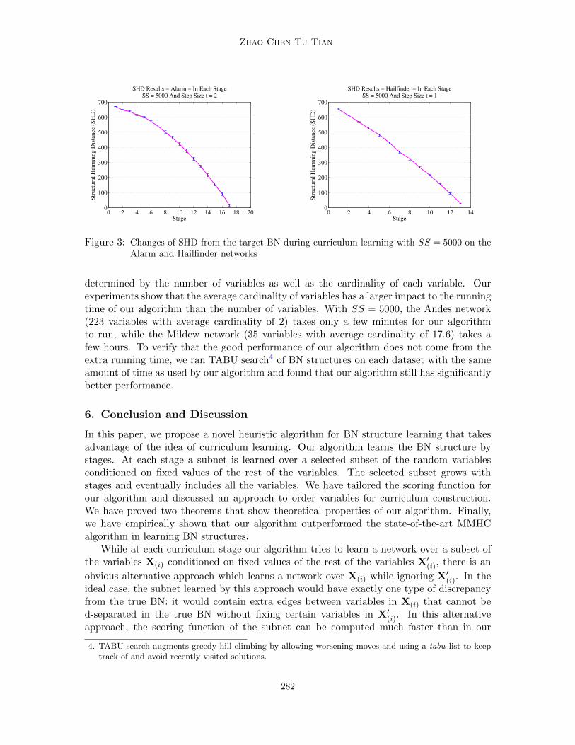
and X′(i). In order to correctly measure the distances between the intermediate learningresults and the target BN, we first randomly generated a fully connected BN over all thevariables, and then at each stage i we replaced the local structure over X(i) with the subnetthat we have learned. Figure 3 plots the SHD between the intermediate learning result ateach stage and the target BN on two different networks. It can be seen that the intermediatelearning results indeed become closer to the learning target with more curriculum stages.

With respect to running-time, our algorithm is in general slower than MMHC, on averagetaking 2.7 times as much time. One reason is that our algorithm has to perform hillclimbing for multiple times, once at each stage, and the number of stages is proportionalto the number of variables. Another reason is that our scoring function takes more timeto compute: we have to compute a separate score for each data segment, which becomesslow when the data is partitioned into too many segments. The number of segments is

281

Zhao Chen Tu Tian

0 2 4 6 8 10 12 14 16 18 200

100

200

300

400

500

600

700

Stage

Str

uct

ura

l H

amm

ing D

ista

nce

(S

HD

)SHD Results − Alarm − In Each Stage

SS = 5000 And Step Size t = 2

0 2 4 6 8 10 12 140

100

200

300

400

500

600

700

Stage

Str

uct

ura

l H

amm

ing D

ista

nce

(S

HD

)

SHD Results − Hailfinder − In Each StageSS = 5000 And Step Size t = 1

Figure 3: Changes of SHD from the target BN during curriculum learning with SS = 5000 on theAlarm and Hailfinder networks

determined by the number of variables as well as the cardinality of each variable. Ourexperiments show that the average cardinality of variables has a larger impact to the runningtime of our algorithm than the number of variables. With SS = 5000, the Andes network(223 variables with average cardinality of 2) takes only a few minutes for our algorithmto run, while the Mildew network (35 variables with average cardinality of 17.6) takes afew hours. To verify that the good performance of our algorithm does not come from theextra running time, we ran TABU search4 of BN structures on each dataset with the sameamount of time as used by our algorithm and found that our algorithm still has significantlybetter performance.

6. Conclusion and Discussion

In this paper, we propose a novel heuristic algorithm for BN structure learning that takesadvantage of the idea of curriculum learning. Our algorithm learns the BN structure bystages. At each stage a subnet is learned over a selected subset of the random variablesconditioned on fixed values of the rest of the variables. The selected subset grows withstages and eventually includes all the variables. We have tailored the scoring function forour algorithm and discussed an approach to order variables for curriculum construction.We have proved two theorems that show theoretical properties of our algorithm. Finally,we have empirically shown that our algorithm outperformed the state-of-the-art MMHCalgorithm in learning BN structures.

While at each curriculum stage our algorithm tries to learn a network over a subset ofthe variables X(i) conditioned on fixed values of the rest of the variables X′(i), there is an

obvious alternative approach which learns a network over X(i) while ignoring X′(i). In theideal case, the subnet learned by this approach would have exactly one type of discrepancyfrom the true BN: it would contain extra edges between variables in X(i) that cannot bed-separated in the true BN without fixing certain variables in X′(i). In this alternativeapproach, the scoring function of the subnet can be computed much faster than in our

4. TABU search augments greedy hill-climbing by allowing worsening moves and using a tabu list to keeptrack of and avoid recently visited solutions.

282

Curriculum Learning of Bayesian Network Structures

original algorithm because no data partition is involved and hence we only need to computea single score. However, the theoretical guarantees given in Theorem 2 and 3 are no longertrue because counter-examples exist. Our experiments also showed that this approach ingeneral resulted in worse learning accuracy than our original algorithm.

References

Silvia Acid and Luis M de Campos. A hybrid methodology for learning belief networks:Benedict. International Journal of Approximate Reasoning, 27(3):235–262, 2001.

Constantin F Aliferis, Ioannis Tsamardinos, Alexander R Statnikov, and Laura E Brown.Causal explorer: A causal probabilistic network learning toolkit for biomedical discovery.In METMBS, volume 3, pages 371–376, 2003.

Eugene L Allgower and Kurt Georg. Numerical continuation methods, volume 13. Springer-Verlag Berlin, 1990.

Mark Bartlett and James Cussens. Advances in Bayesian network learning using integerprogramming. In Proceedings of the 29th Conference on Uncertainty in Artificial Intelli-gence (UAI-13), pages 182–191, 2013.

Yoshua Bengio, Jerome Louradour, Ronan Collobert, and Jason Weston. Curriculum learn-ing. In Proceedings of the 26th annual international conference on machine learning,pages 41–48. ACM, 2009.

David Maxwell Chickering. Learning Bayesian networks is NP-complete. In Learning fromdata, pages 121–130. Springer, 1996.

Gregory F Cooper and Edward Herskovits. A Bayesian method for the induction of prob-abilistic networks from data. Machine learning, 9(4):309–347, 1992.

I Csisz et al. Information-type measures of difference of probability distributions and indirectobservations. Studia Sci. Math. Hungar., 2:299–318, 1967.

Jeffrey L. Elman. Learning and development in neural networks: The importance of startingsmall. Cognition, 48:71–99, 1993.

David Heckerman, Dan Geiger, and David M Chickering. Learning bayesian networks: Thecombination of knowledge and statistical data. Machine learning, 20(3):197–243, 1995.

Tommi Jaakkola, David Sontag, Amir Globerson, and Marina Meila. Learning Bayesian net-work structure using lp relaxations. In International Conference on Artificial Intelligenceand Statistics, pages 358–365, 2010.

Lu Jiang, Deyu Meng, Qian Zhao, Shiguang Shan, and Alexander G Hauptmann. Self-pacedcurriculum learning. In Twenty-Ninth AAAI Conference on Artificial Intelligence, 2015.

Mikko Koivisto and Kismat Sood. Exact Bayesian structure discovery in Bayesian networks.The Journal of Machine Learning Research, 5:549–573, 2004.

283

Zhao Chen Tu Tian

M. Pawan Kumar, Benjamin Packer, and Daphne Koller. Self-paced learning for latentvariable models. In Advances in Neural Information Processing Systems 23. 2010.

Brandon Malone, Matti Jarvisalo, and Petri Myllymaki. Impact of learning strategies onthe quality of Bayesian networks: An empirical evaluation. In Proceedings of the 31stConference on Uncertainty in Artificial Intelligence (UAI 2015), 2015.

Brandon M Malone, Changhe Yuan, and Eric A Hansen. Memory-efficient dynamic pro-gramming for learning optimal Bayesian networks. In AAAI, 2011.

D. Margaritis and S. Thrun. Bayesian network induction via local neighborhoods. InAdvances in Neural Information Processing Systems 12, pages 505–511. MIT Press, 2000.

Judea Pearl. Causality: models, reasoning and inference, volume 29. Cambridge Univ Press,2000.

Jean-Philippe Pellet and Andre Elisseeff. Using markov blankets for causal structure learn-ing. The Journal of Machine Learning Research, 9:1295–1342, 2008.

Tomi Silander and Petri Myllymaki. A simple approach for finding the globally optimalBayesian network structure. In Proceedings of the 22th Conference on Uncertainty inArtificial Intelligence, pages 445–452, 2006.

Peter Spirtes, Clark Glymour, and Richard Scheines. Causation, prediction, and search.MIT Press, 2001.

Valentin I. Spitkovsky, Hiyan Alshawi, and Daniel Jurafsky. From baby steps to leapfrog:How “less is more” in unsupervised dependency parsing. In NAACL, 2010.

Ioannis Tsamardinos, Constantin F Aliferis, and Alexander Statnikov. Time and sampleefficient discovery of markov blankets and direct causal relations. In Proceedings of theninth ACM SIGKDD international conference on Knowledge discovery and data mining,pages 673–678. ACM, 2003.

Ioannis Tsamardinos, Laura E Brown, and Constantin F Aliferis. The max-min hill-climbingBayesian network structure learning algorithm. Machine learning, 65(1):31–78, 2006.

Kewei Tu and Vasant Honavar. On the utility of curricula in unsupervised learning of prob-abilistic grammars. In IJCAI Proceedings-International Joint Conference on ArtificialIntelligence, volume 22, page 1523, 2011.

Thomas Verma and Judea Pearl. Equivalence and synthesis of causal models. In Proceedingsof the Sixth Annual Conference on Uncertainty in Artificial Intelligence, 1990.

Changhe Yuan and Brandon Malone. An improved admissible heuristic for learning optimalBayesian networks. In Proceedings of the 28th Conference on Uncertainty in ArtificialIntelligence (UAI-12), 2012.

Changhe Yuan, Brandon Malone, and Xiaojian Wu. Learning optimal Bayesian networksusing a* search. In Proceedings of the Twenty-Second international joint conference onArtificial Intelligence, pages 2186–2191, 2011.

284