Curvature of Metric Spaces

John LottUniversity of Michigan

http://www.math.lsa.umich.edu/˜lott

May 23, 2007

Special Session on Metric Differential Geometry

Thursday, Friday, Saturday morning

Joint work with Cedric Villani.

Related work was done independently by K.-T. Sturm.

Special Session on Metric Differential Geometry

Thursday, Friday, Saturday morning

Joint work with Cedric Villani.

Related work was done independently by K.-T. Sturm.

Curvature of Metric Spaces

Introduction

Five minute summary of differential geometry

Metric geometry

Alexandrov curvature

Optimal transport

Entropy functionals

Abstract Ricci curvature

Applications

Introduction

Goal : We have notions of curvature from differential geometry.

Do they make sense for metric spaces?

For example, does it make sense to say that a metric space is“positively curved”?

Motivations :1. Intrinsic interest2. Understanding3. Applications to smooth geometry

Introduction

Goal : We have notions of curvature from differential geometry.

Do they make sense for metric spaces?

For example, does it make sense to say that a metric space is“positively curved”?

Motivations :1. Intrinsic interest2. Understanding3. Applications to smooth geometry

Curvature of Metric Spaces

Introduction

Five minute summary of differential geometry

Metric geometry

Alexandrov curvature

Optimal transport

Entropy functionals

Abstract Ricci curvature

Applications

Length structure of a Riemannian manifold

Say M is a smooth n-dimensional manifold. For each m ∈ M,the tangent space TmM is an n-dimensional vector space.

A Riemannian metric g on M assigns, to each m ∈ M, an innerproduct on TmM.

Example : M is a submanifold of RN

If v ∈ TmM, let g(v, v) be the square of the length of v.

Length structure of a Riemannian manifold

Say M is a smooth n-dimensional manifold. For each m ∈ M,the tangent space TmM is an n-dimensional vector space.

A Riemannian metric g on M assigns, to each m ∈ M, an innerproduct on TmM.

Example : M is a submanifold of RN

If v ∈ TmM, let g(v, v) be the square of the length of v.

Length structure of a Riemannian manifold

The length of a smooth curve γ : [0, 1] → M is

L(γ) =

∫ 1

0

√g(γ, γ) dt .

The distance between m0, m1 ∈ M is the infimal length ofcurves joining m0 to m1.

Length structure of a Riemannian manifold

d(m0, m1) = inf{L(γ) : γ(0) = m0, γ(1) = m1}.

Fact : this defines a metric on the set M.

Any length-minimizing curve from m0 to m1 is a geodesic.

Riemannian volume

Any Riemannian manifold M comes equipped with a smoothpositive measure dvolM .

In local coordinates, if g =∑n

i,j=1 gij dx i dx j then

dvolM =√

det (gij) dx1dx2 . . . dxn.

The volume of a nice subset A ⊂ M is

vol(A) =

∫A

dvolM .

Sectional curvature

To each m ∈ M and each 2-plane P ⊂ TmM in the tangentspace at m, one assigns a number K (P), its sectionalcurvature.

Example : If M is two-dimensional then P is all of TmM andK (P) is the Gaussian curvature at m.

Sectional curvature

To each m ∈ M and each 2-plane P ⊂ TmM in the tangentspace at m, one assigns a number K (P), its sectionalcurvature.

Example : If M is two-dimensional then P is all of TmM andK (P) is the Gaussian curvature at m.

Ricci curvature

Ricci curvature is an averaging of sectional curvature.

Fix a unit-length vector v ∈ TmM.

Definition

Ric(v, v) = (n − 1) · (the average sectional curvature

of the 2-planes P containing v).

Example : S2 × S2 ⊂ (R3 × R3 = R6) has nonnegativesectional curvatures but has positive Ricci curvatures.

Ricci curvature

Ricci curvature is an averaging of sectional curvature.

Fix a unit-length vector v ∈ TmM.

Definition

Ric(v, v) = (n − 1) · (the average sectional curvature

of the 2-planes P containing v).

Example : S2 × S2 ⊂ (R3 × R3 = R6) has nonnegativesectional curvatures but has positive Ricci curvatures.

Ricci curvature

What does Ricci curvature control?

1. Volume growth

Bishop-Gromov inequality :If M has nonnegative Ricci curvature then balls in M grow nofaster than in Euclidean space.

That is, for any m ∈ M, r−n vol(Br (m)) is nonincreasing in r .

2. The universe

Einstein says that a matter-free spacetime has vanishing Riccicurvature.

Ricci curvature

What does Ricci curvature control?

1. Volume growth

Bishop-Gromov inequality :If M has nonnegative Ricci curvature then balls in M grow nofaster than in Euclidean space.

That is, for any m ∈ M, r−n vol(Br (m)) is nonincreasing in r .

2. The universe

Einstein says that a matter-free spacetime has vanishing Riccicurvature.

Summary

Any Riemannian manifold gets

1. Lengths of curves2. A metric space structure3. A measure4. Sectional curvatures5. Ricci curvatures

Question :To what extent can we recover the sectional curvatures fromjust the metric space structure?

To what extent can we recover the Ricci curvatures from justthe metric space structure and the measure?

Summary

Any Riemannian manifold gets

1. Lengths of curves2. A metric space structure3. A measure4. Sectional curvatures5. Ricci curvatures

Question :To what extent can we recover the sectional curvatures fromjust the metric space structure?

To what extent can we recover the Ricci curvatures from justthe metric space structure and the measure?

Curvature of Metric Spaces

Introduction

Five minute summary of differential geometry

Metric geometry

Alexandrov curvature

Optimal transport

Entropy functionals

Abstract Ricci curvature

Applications

Length spaces

Say (X , d) is a compact metric space and γ : [0, 1] → X is acontinuous map.

The length of γ is

L(γ) = supJ

sup0=t0≤t1≤...≤tJ=1

J∑j=1

d(γ(tj−1), γ(tj)).

Length spaces

Say (X , d) is a compact metric space and γ : [0, 1] → X is acontinuous map.

The length of γ is

L(γ) = supJ

sup0=t0≤t1≤...≤tJ=1

J∑j=1

d(γ(tj−1), γ(tj)).

Length spaces

(X , d) is a length space if the distance between two pointsx0, x1 ∈ X equals the infimum of the lengths of curves joiningthem, i.e.

d(x0, x1) = inf{L(γ) : γ(0) = x0, γ(1) = x1}.

A length-minimizing curve is called a geodesic.

Length spaces

(X , d) is a length space if the distance between two pointsx0, x1 ∈ X equals the infimum of the lengths of curves joiningthem, i.e.

d(x0, x1) = inf{L(γ) : γ(0) = x0, γ(1) = x1}.

A length-minimizing curve is called a geodesic.

Length spaces

Examples of length spaces :1. The underlying metric space of any Riemannian manifold.2.

Nonexamples :1. A finite metric space with more than one point.2. A circle with the chordal metric.

Length spaces

Examples of length spaces :1. The underlying metric space of any Riemannian manifold.2.

Nonexamples :1. A finite metric space with more than one point.2. A circle with the chordal metric.

Curvature of Metric Spaces

Introduction

Five minute summary of differential geometry

Metric geometry

Alexandrov curvature

Optimal transport

Entropy functionals

Abstract Ricci curvature

Applications

Alexandrov curvature

DefinitionA compact length space (X , d) has nonnegative Alexandrovcurvature if geodesic triangles in X are at least as “fat” ascorresponding triangles in R2.

The comparison triangle in R2 has the same sidelengthsFatness :(Length of bisector from x) ≥ (Length of bisector from x0)

Alexandrov curvature

DefinitionA compact length space (X , d) has nonnegative Alexandrovcurvature if geodesic triangles in X are at least as “fat” ascorresponding triangles in R2.

The comparison triangle in R2 has the same sidelengthsFatness :(Length of bisector from x) ≥ (Length of bisector from x0)

Alexandrov curvature

Example : the boundary of a convex region in RN hasnonnegative Alexandrov curvature.

1. If (M, g) is a Riemannian manifold then its underlying metricspace has nonnegative Alexandrov curvature if and only if Mhas nonnegative sectional curvatures.

2. If {(Xi , di)}∞i=1 have nonnegative Alexandrov curvature andlimi→∞(Xi , di) = (X , d) in the Gromov-Hausdorff topology then(X , d) has nonnegative Alexandrov curvature.

3. Applications to Riemannian geometry

Alexandrov curvature

Example : the boundary of a convex region in RN hasnonnegative Alexandrov curvature.

1. If (M, g) is a Riemannian manifold then its underlying metricspace has nonnegative Alexandrov curvature if and only if Mhas nonnegative sectional curvatures.

2. If {(Xi , di)}∞i=1 have nonnegative Alexandrov curvature andlimi→∞(Xi , di) = (X , d) in the Gromov-Hausdorff topology then(X , d) has nonnegative Alexandrov curvature.

3. Applications to Riemannian geometry

Gromov-Hausdorff topology

A topology on the set of all compact metric spaces (moduloisometry).

(X1, d1) and (X2, d2) are close in the Gromov-Hausdorfftopology if somebody with bad vision has trouble telling themapart.

Example : a cylinder with a small cross-section isGromov-Hausdorff close to a line segment.

Gromov-Hausdorff topology

A topology on the set of all compact metric spaces (moduloisometry).

(X1, d1) and (X2, d2) are close in the Gromov-Hausdorfftopology if somebody with bad vision has trouble telling themapart.

Example : a cylinder with a small cross-section isGromov-Hausdorff close to a line segment.

The question

Can one extend Alexandrov’s work from sectional curvature toRicci curvature?

Motivation : Gromov’s precompactness theorem

TheoremGiven N ∈ Z+ and D > 0,

{(M, g) : dim(M) = N, diam(M) ≤ D, RicM ≥ 0}

is precompact in the Gromov-Hausdorff topology on{compact metric spaces}/isometry.

Gromov-Hausdorff space

Each point is a compact metric space.Each interior point is a Riemannian manifold (M, g) withdim(M) = N, diam(M) ≤ D and RicM ≥ 0.

The boundary points are compact metric spaces (X , d) withdimH X ≤ N. They are generally not manifolds.(Example : X = M/G.)

In some moral sense, the boundary points are metric spaceswith “nonnegative Ricci curvature”.

Gromov-Hausdorff space

Each point is a compact metric space.Each interior point is a Riemannian manifold (M, g) withdim(M) = N, diam(M) ≤ D and RicM ≥ 0.

The boundary points are compact metric spaces (X , d) withdimH X ≤ N. They are generally not manifolds.(Example : X = M/G.)

In some moral sense, the boundary points are metric spaceswith “nonnegative Ricci curvature”.

Curvature of Metric Spaces

Introduction

Five minute summary of differential geometry

Metric geometry

Alexandrov curvature

Optimal transport

Entropy functionals

Abstract Ricci curvature

Applications

Dirtmoving

Given a before and an after dirtpile, what is the most efficientway to move the dirt from one place to the other?

Let’s say that the cost to move a gram of dirt from x to y isd(x , y)2.

Gaspard Monge

Memoire sur la theorie des deblais et des remblais (1781)

Memoir on the theory of excavations and fillings (1781)

Gaspard Monge

Wasserstein space

Let (X , d) be a compact metric space.

NotationP(X ) is the set of Borel probability measures on X.

That is, µ ∈ P(X ) iff µ is a nonnegative Borel measure on Xwith µ(X ) = 1.

DefinitionGiven µ0, µ1 ∈ P(X ), the Wasserstein distance W2(µ0, µ1) isthe square root of the minimal cost to transport µ0 to µ1.

Wasserstein space

W2(µ0, µ1)2 = inf

{∫X×X

d(x , y)2 dπ(x , y)

},

where

π ∈ P(X × X ), (p0)∗π = µ0, (p1)∗π = µ1.

Wasserstein space

Fact :(P(X ), W2) is a metric space, called the Wasserstein space.

The metric topology is the weak-∗ topology, i.e. limi→∞ µi = µ ifand only if for all f ∈ C(X ), limi→∞

∫X f dµi =

∫X f dµ.

PropositionIf X is a length space then so is the Wasserstein space P(X ).

Hence we can talk about its (minimizing) geodesics {µt}t∈[0,1],called Wasserstein geodesics.

Wasserstein space

Fact :(P(X ), W2) is a metric space, called the Wasserstein space.

The metric topology is the weak-∗ topology, i.e. limi→∞ µi = µ ifand only if for all f ∈ C(X ), limi→∞

∫X f dµi =

∫X f dµ.

PropositionIf X is a length space then so is the Wasserstein space P(X ).

Hence we can talk about its (minimizing) geodesics {µt}t∈[0,1],called Wasserstein geodesics.

Optimal transport

What is the optimal transport scheme between µ0, µ1 ∈ P(X )?

X = Rn, µ0 and µ1 absolutely continuous :Rachev-Ruschendorf, Brenier (1990)

X a Riemannian manifold, µ0 and µ1 absolutely continuous :McCann (2001)

Empirical fact : The Ricci curvature of the Riemannian manifoldaffects the optimal transport in a quantitative way.Otto-Villani (2000),Cordero-Erausquin-McCann-Schmuckenschlager (2001)

Metric-measure spaces

DefinitionA metric-measure space is a metric space (X , d) equipped witha given probability measure ν ∈ P(X ).

A smooth metric-measure space is a Riemannian manifold(M, g) with a smooth probability measure dν = e−Ψ dvolM .

Idea : Use optimal transport on X to define what it means for(X , ν) to have “nonnegative Ricci curvature”.

(X , d) −→ (P(X ), W2)To one compact length space we have assigned another.Use the properties of the Wasserstein space (P(X ), W2) to saysomething about the geometry of (X , d).

Metric-measure spaces

DefinitionA metric-measure space is a metric space (X , d) equipped witha given probability measure ν ∈ P(X ).

A smooth metric-measure space is a Riemannian manifold(M, g) with a smooth probability measure dν = e−Ψ dvolM .

Idea : Use optimal transport on X to define what it means for(X , ν) to have “nonnegative Ricci curvature”.

(X , d) −→ (P(X ), W2)To one compact length space we have assigned another.Use the properties of the Wasserstein space (P(X ), W2) to saysomething about the geometry of (X , d).

Measured Gromov-Hausdorff limits

An easy consequence of Gromov precompactness :{(M, g,

dvolMvol(M)

): dim(M) = N, diam(M) ≤ D, RicM ≥ 0

}is precompact in the measured Gromov-Hausdorff topology on{compact metric-measure spaces}/isometry.

What can we say about the limit points? (Work ofCheeger-Colding)

What are the smooth limit points?

Measured Gromov-Hausdorff limits

An easy consequence of Gromov precompactness :{(M, g,

dvolMvol(M)

): dim(M) = N, diam(M) ≤ D, RicM ≥ 0

}is precompact in the measured Gromov-Hausdorff topology on{compact metric-measure spaces}/isometry.

What can we say about the limit points? (Work ofCheeger-Colding)

What are the smooth limit points?

Measured Gromov-Hausdorff (MGH) topology

Definitionlimi→∞(Xi , di , νi) = (X , d , ν) if there are Borel mapsfi : Xi → X and a sequence εi → 0 such that1. (Almost isometry) For all xi , x ′i ∈ Xi ,

|dX (fi(xi), fi(x′i ))− dXi

(xi , x ′i )| ≤ εi .

2. (Almost surjective) For all x ∈ X and all i , there is somexi ∈ Xi such that

dX (fi(xi), x) ≤ εi .

3. limi→∞(fi)∗νi = ν in the weak-∗ topology.

Curvature of Metric Spaces

Introduction

Five minute summary of differential geometry

Metric geometry

Alexandrov curvature

Optimal transport

Entropy functionals

Abstract Ricci curvature

Applications

Notation

X a compact Hausdorff space.

P(X ) = Borel probability measures on X , with weak-∗ topology.

U : [0,∞) → R a continuous convex function with U(0) = 0.

Fix a background measure ν ∈ P(X ).

Entropy

The “negative entropy” of µ with respect to ν is

Uν(µ) =

∫X

U(ρ(x)) dν(x) + U ′(∞) µs(X ).

Hereµ = ρ ν + µs

is the Lebesgue decomposition of µ with respect to ν and

U ′(∞) = limr→∞

U(r)r

.

Uν(µ) measures the nonuniformity of µ w.r.t. ν. It is minimizedwhen µ = ν.

We get a function Uν : P(X ) → R ∪∞.

Entropy

The “negative entropy” of µ with respect to ν is

Uν(µ) =

∫X

U(ρ(x)) dν(x) + U ′(∞) µs(X ).

Hereµ = ρ ν + µs

is the Lebesgue decomposition of µ with respect to ν and

U ′(∞) = limr→∞

U(r)r

.

Uν(µ) measures the nonuniformity of µ w.r.t. ν. It is minimizedwhen µ = ν.

We get a function Uν : P(X ) → R ∪∞.

Effective dimension

N ∈ [1,∞] a new parameter (possibly infinite).

It turns out that there’s not a single notion of “nonnegative Riccicurvature”, but rather a 1-parameter family. That is, for each N,there’s a notion of a space having “nonnegative N-Riccicurvature”.

Here N is an effective dimension of the space, and must beinputted.

Displacement convexity classes

Definition(McCann) If N < ∞ then DCN is the set of such convexfunctions U so that the function

λ → λN U(λ−N)

is convex on (0,∞).

DefinitionDC∞ is the set of such convex functions U so that the function

λ → eλ U(e−λ)

is convex on (−∞,∞).

Displacement convexity classes

Example

UN(r) =

{Nr(1− r−1/N) if 1 < N < ∞,

r log r if N = ∞.

If U = U∞ then the corresponding functional is

Uν(µ) =

{∫X ρ log ρ dν if µ is a.c. w.r.t. ν,

∞ otherwise,

where µ = ρ ν.

Curvature of Metric Spaces

Introduction

Five minute summary of differential geometry

Metric geometry

Alexandrov curvature

Optimal transport

Entropy functionals

Abstract Ricci curvature

Applications

Convexity on Wasserstein space

(X , d) is a compact length space.

ν is a fixed probability measure on X .

We want to ask whether the negative entropy function Uν is aconvex function on P(X ).

That is, given µ0, µ1 ∈ P(X ), whether Uν restricts to a convexfunction along a Wasserstein geodesic {µt}t∈[0,1] from µ0 to µ1.

Convexity on Wasserstein space

(X , d) is a compact length space.

ν is a fixed probability measure on X .

We want to ask whether the negative entropy function Uν is aconvex function on P(X ).

That is, given µ0, µ1 ∈ P(X ), whether Uν restricts to a convexfunction along a Wasserstein geodesic {µt}t∈[0,1] from µ0 to µ1.

Nonnegative N-Ricci curvature

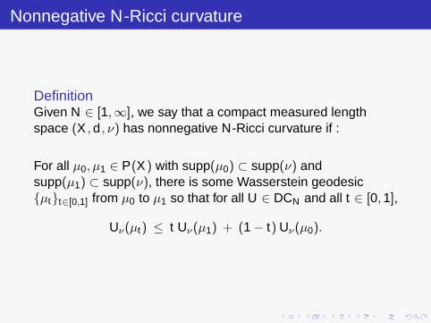
DefinitionGiven N ∈ [1,∞], we say that a compact measured lengthspace (X , d , ν) has nonnegative N-Ricci curvature if :

For all µ0, µ1 ∈ P(X ) with supp(µ0) ⊂ supp(ν) andsupp(µ1) ⊂ supp(ν), there is some Wasserstein geodesic{µt}t∈[0,1] from µ0 to µ1 so that for all U ∈ DCN and all t ∈ [0, 1],

Uν(µt) ≤ t Uν(µ1) + (1− t) Uν(µ0).

Nonnegative N-Ricci curvature

Note : We only require convexity along some geodesic from µ0

to µ1, not all geodesics.

But the same geodesic has to work for all U ∈ DCN .

What does this have to do with curvature?

Look at optimal transport on the 2-sphere.ν = normalized Riemannian density.Take µ0, µ1 two disjoint congruent blobs. Uν(µ0) = Uν(µ1).

Optimal transport from µ0 to µ1 goes along longitudes.Positive curvature gives focusing of geodesics.

What does this have to do with curvature?

Look at optimal transport on the 2-sphere.ν = normalized Riemannian density.Take µ0, µ1 two disjoint congruent blobs. Uν(µ0) = Uν(µ1).

Optimal transport from µ0 to µ1 goes along longitudes.Positive curvature gives focusing of geodesics.

Take a snapshot at time t .

The intermediate-time blob µt is more spread out, so it’s moreuniform with respect to ν.The more uniform the measure, the higher its entropy.So the entropy is a concave function of t , i.e. the negativeentropy is a convex function of t .

Take a snapshot at time t .

The intermediate-time blob µt is more spread out, so it’s moreuniform with respect to ν.The more uniform the measure, the higher its entropy.

So the entropy is a concave function of t , i.e. the negativeentropy is a convex function of t .

Take a snapshot at time t .

The intermediate-time blob µt is more spread out, so it’s moreuniform with respect to ν.The more uniform the measure, the higher its entropy.So the entropy is a concave function of t , i.e. the negativeentropy is a convex function of t .

Main result

TheoremLet {(Xi , di , νi)}∞i=1 be a sequence of compact measured lengthspaces with

limi→∞

(Xi , di , νi) = (X , d , ν)

in the measured Gromov-Hausdorff topology.

For any N ∈ [1,∞], if each (Xi , di , νi) has nonnegative N-Riccicurvature then (X , d , ν) has nonnegative N-Ricci curvature.

What does all this have to do with Ricci curvature?

Let (M, g) be a compact connected n-dimensional Riemannianmanifold.We could take the Riemannian measure, but let’s be moregeneral.

Say Ψ ∈ C∞(M) has ∫M

e−Ψ dvolM = 1.

Put ν = e−Ψ dvolM .

Any smooth positive probability measure on M can be written inthis way.

What does all this have to do with Ricci curvature?

Let (M, g) be a compact connected n-dimensional Riemannianmanifold.We could take the Riemannian measure, but let’s be moregeneral.

Say Ψ ∈ C∞(M) has ∫M

e−Ψ dvolM = 1.

Put ν = e−Ψ dvolM .

Any smooth positive probability measure on M can be written inthis way.

What does all this have to do with Ricci curvature?

For N ∈ [1,∞], define the N-Ricci tensor RicN of (Mn, g, ν) byRic + Hess(Ψ) if N = ∞,

Ric + Hess(Ψ) − 1N−n dΨ⊗ dΨ if n < N < ∞,

Ric + Hess(Ψ) − ∞ (dΨ⊗ dΨ) if N = n,

−∞ if N < n,

where by convention ∞ · 0 = 0.

RicN is a symmetric covariant 2-tensor field on M that dependson g and Ψ.

(If N = n then RicN is −∞ except where dΨ = 0. There,RicN = Ric.)

Ric∞ = Bakry-Emery tensor = right-hand side of Perelman’smodified Ricci flow equation.

What does all this have to do with Ricci curvature?

For N ∈ [1,∞], define the N-Ricci tensor RicN of (Mn, g, ν) byRic + Hess(Ψ) if N = ∞,

Ric + Hess(Ψ) − 1N−n dΨ⊗ dΨ if n < N < ∞,

Ric + Hess(Ψ) − ∞ (dΨ⊗ dΨ) if N = n,

−∞ if N < n,

where by convention ∞ · 0 = 0.

RicN is a symmetric covariant 2-tensor field on M that dependson g and Ψ.

(If N = n then RicN is −∞ except where dΨ = 0. There,RicN = Ric.)

Ric∞ = Bakry-Emery tensor = right-hand side of Perelman’smodified Ricci flow equation.

Abstract Ricci recovers classical Ricci

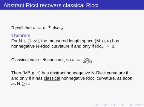
Recall that ν = e−Ψ dvolM .

TheoremFor N ∈ [1,∞], the measured length space (M, g, ν) hasnonnegative N-Ricci curvature if and only if RicN ≥ 0.

Classical case : Ψ constant, so ν = dvolvol(M) .

Then (Mn, g, ν) has abstract nonnegative N-Ricci curvature ifand only if it has classical nonnegative Ricci curvature, as soonas N ≥ n.

Abstract Ricci recovers classical Ricci

Recall that ν = e−Ψ dvolM .

TheoremFor N ∈ [1,∞], the measured length space (M, g, ν) hasnonnegative N-Ricci curvature if and only if RicN ≥ 0.

Classical case : Ψ constant, so ν = dvolvol(M) .

Then (Mn, g, ν) has abstract nonnegative N-Ricci curvature ifand only if it has classical nonnegative Ricci curvature, as soonas N ≥ n.

Curvature of Metric Spaces

Introduction

Five minute summary of differential geometry

Metric geometry

Alexandrov curvature

Optimal transport

Entropy functionals

Abstract Ricci curvature

Applications

Smooth limit spaces

Had Gromov precompactness theorem. What are the limitspaces (X , d , ν)? Suppose that the limit space is a smoothmeasured length space, i.e.

(X , d , ν) = (B, gB, e−Ψ dvolB)

for some n-dimensional smooth Riemannian manifold (B, gB)and some Ψ ∈ C∞(B).

TheoremIf (B, gB, e−Ψ dvolB) is a measured Gromov-Hausdorff limit ofRiemannian manifolds with nonnegative Ricci curvature anddimension at most N then RicN(B) ≥ 0.

Note : the dimension can drop on taking limits.

The converse is true if N ≥ n + 2.

Smooth limit spaces

Had Gromov precompactness theorem. What are the limitspaces (X , d , ν)? Suppose that the limit space is a smoothmeasured length space, i.e.

(X , d , ν) = (B, gB, e−Ψ dvolB)

for some n-dimensional smooth Riemannian manifold (B, gB)and some Ψ ∈ C∞(B).

TheoremIf (B, gB, e−Ψ dvolB) is a measured Gromov-Hausdorff limit ofRiemannian manifolds with nonnegative Ricci curvature anddimension at most N then RicN(B) ≥ 0.

Note : the dimension can drop on taking limits.

The converse is true if N ≥ n + 2.

Smooth limit spaces

Had Gromov precompactness theorem. What are the limitspaces (X , d , ν)? Suppose that the limit space is a smoothmeasured length space, i.e.

(X , d , ν) = (B, gB, e−Ψ dvolB)

for some n-dimensional smooth Riemannian manifold (B, gB)and some Ψ ∈ C∞(B).

TheoremIf (B, gB, e−Ψ dvolB) is a measured Gromov-Hausdorff limit ofRiemannian manifolds with nonnegative Ricci curvature anddimension at most N then RicN(B) ≥ 0.

Note : the dimension can drop on taking limits.

The converse is true if N ≥ n + 2.

Bishop-Gromov-type inequality

TheoremIf (X , d , ν) has nonnegative N-Ricci curvature and x ∈ supp(ν)then r−N ν(Br (x)) is nonincreasing in r .

Lichnerowicz inequality

If (M, g) is a compact Riemannian manifold, let λ1 be thesmallest positive eigenvalue of the Laplacian −∇2.

TheoremLichnerowicz (1964)If dim(M) = n and M has Ricci curvatures bounded below byK > 0 then

λ1 ≥n

n − 1K .

Sharp global Poincare inequality

TheoremIf (X , d , ν) has N-Ricci curvature bounded below by K > 0 andf is a Lipschitz function on X with

∫X f dν = 0 then∫

Xf 2 dν ≤ N − 1

N1K

∫X|∇f |2 dν.

Here

|∇f |(x) = lim supy→x

|f (y)− f (x)|d(y , x)

.

Sharp global Poincare inequality

TheoremIf (X , d , ν) has N-Ricci curvature bounded below by K > 0 andf is a Lipschitz function on X with

∫X f dν = 0 then∫

Xf 2 dν ≤ N − 1

N1K

∫X|∇f |2 dν.

Here

|∇f |(x) = lim supy→x

|f (y)− f (x)|d(y , x)

.

Open questions

1. Take any result that you know about Riemannian manifoldswith nonnegative Ricci curvature.

Does it extend to measured length spaces (X , d , ν) withnonnegative N-Ricci curvature?(Yes for Bishop-Gromov, no for splitting theorem.)

2. Take an interesting measured length space (X , d , ν). Does ithave nonnegative N-Ricci curvature?

This almost always boils down to understanding the optimaltransport on X .