Submitted 21 December 2016Accepted 17 February 2017Published 22 March 2017

Corresponding authorHazel L. Richards,hazel.l.richards@gmail.com

Academic editorPhilip Cox

Additional Information andDeclarations can be found onpage 14

DOI 10.7717/peerj.3100

Copyright2017 McCabe et al.

Distributed underCreative Commons CC-BY 4.0

OPEN ACCESS

Curvature reduces bending strains in thequokka femurKyle McCabe, Keith Henderson, Jess Pantinople, Hazel L. Richards andNick MilneSchool of Anatomy, Physiology and Human Biology, University of Western Australia, Perth, WesternAustralia, Australia

ABSTRACTThis study explores how curvature in the quokka femur may help to reduce bendingstrain during locomotion. The quokka is a small wallaby, but the curvature of the femurand the muscles active during stance phase are similar to most quadrupedal mammals.Our hypothesis is that the action of hip extensor and ankle plantarflexormuscles duringstance phase place cranial bending strains that act to reduce the caudal curvature ofthe femur. Knee extensors and biarticular muscles that span the femur longitudinallycreate caudal bending strains in the caudally curved (concave caudal side) bone. Theseopposing strains can balance each other and result in less strain on the bone. We testthis idea by comparing the performance of a normally curved finite element model ofthe quokka femur to a digitally straightened version of the same bone. The normallycurved model is indeed less strained than the straightened version. To further examinethe relationship between curvature and the strains in the femoral models, we also testedan extra-curved and a reverse-curved version with the same loads. There appears to bea linear relationship between the curvature and the strains experienced by the models.These results demonstrate that longitudinal curvature in bones may be a manipulablemechanism whereby bone can induce a strain gradient to oppose strains induced byhabitual loading.

Subjects Computational Biology, Evolutionary Studies, ZoologyKeywords Femur, Finite elements analysis, Curved bones, Strain reduction

INTRODUCTIONMany long bones in animal limbs are curved, but such curvature is thought to reduce thebones strength under longitudinal loading. Several authors have constructed hypotheses toexplain this apparent paradox of bone curvature. It has been suggested that curvature mayserve to induce strain (Lanyon, 1980), accommodate musculature (Lanyon, 1980), or warnof impending strain limits (Currey, 1984). The most widely accepted hypothesis suggeststhat bone curvature is the result of a trade-off between strength and predictable bending(Bertram & Biewener, 1988). A curved bone, while not as strong as a straight bone, willonly ever experience unidirectional bending strain. In contrast, straight bones are liable toexperience bending in any direction. While the ‘‘predictability hypothesis’’ is potentiallypowerful, it lacks an operational mechanism.

Frost (1964) and Pauwels (1980) separately suggested that the combination of musclebending and bending due to longitudinal loading of bone curvature serves to moderate

How to cite this article McCabe et al. (2017), Curvature reduces bending strains in the quokka femur. PeerJ 5:e3100; DOI10.7717/peerj.3100

the net strain experienced by bone. Pauwels (1980) demonstrated that bending momentsof equal magnitude but opposite orientation will cancel out, and Frost (1964) proposed acellular mechanism whereby bones may develop curvature as a result of habitual loading.Both authors illustrated their arguments using thought experiments; however, their ideasremained experimentally unvalidated until recently.

Milne (2016), drawing on the ideas of Frost (1964) andPauwels (1980), recently suggestedthat curvature in long bones is a strain-reducing adaptation to habitual loading. A llama(Lama guanicoe) radioulna was used to illustrate this hypothesis. In terrestrial quadrupeds,the action of triceps pulling on the olecranon process exerts a substantial bending load uponthe radioulna simply to maintain stance. This habitual loading induces a cranial-bendingstrain gradient in the bone (tending tomake it cranially concave). Milne used finite elementanalysis to demonstrate that the normally curved llama radioulna is subject to less bendingstrain than a straightened version of the same bone when subject to loading from tricepsand longitudinal forces. He argued that this because the radioulna in these species—indeedin most terrestrial quadrupeds—is caudally curved (with a caudal-facing concavity). Whenthis curvature is subject to longitudinal loading from gravity, joint reaction forces or othermuscular forces, it deforms predictably—it will be subject to caudal bending. The cranialbending due to triceps and the curvature-induced caudal bending are in direct opposition,and so will cancel, leaving the bone in a neutral or reduced bending state.

There have been a number of strain gauge studies examining the radius and tibiaof quadrupedal animals during locomotion (Lanyon & Baggott, 1976; Lanyon & Bourn,1979; Lanyon, Magee & Baggott, 1979; Biewener et al., 1983; Swartz, Bertram & Biewener,1989). Recently Copploe and colleagues (2015) placed strain gauges on the femur ofand armadillo and found predominantly mediolateral bending in the medially (concave)curved armadillo femur. Jade and colleagues (2014) used finite elements analysis to examineBertram & Biewener’s (1988) predictability hypothesis and showed that the caudally curvedhuman femur is placed in caudal bending when subjected to longitudinal loading.

When a terrestrial animal bears weight on its hindlimb, the hip and knee must resistflexion and the ankle must resist dorsiflexion. The active muscles are the hip extensors(hamstrings, quadratus femoris and the adductors), the knee extensors (quadriceps) andthe calf muscles joining the Achilles tendon (Elftman, 1929; Freedman & Twomey, 1979). Atthe beginning of stance these muscles are expected to act eccentrically as the limb absorbsground reaction forces. These muscles continue to act, and work concentrically towardsthe end of stance. The muscles that attach to the posterior aspect of the femur (quadratusfemoris and adductors superiorly, gastrocnemius and plantaris inferiorly) are expected tocause cranial bending (compression on the cranial side). In the caudally-curved femur,the longitudinal forces, hamstrings, and quadriceps are expected to induce caudal bendingforces, thus balancing this cranial bending. However, if the femur were not caudally curved,these longitudinal forces would be less able to counter cranial bending.

This study used finite element analysis to compare the strains in models of the femur of aquokka (Setonix brachyurus) with varying degrees of curvature. A finite element model of anormal femur was warped to produce straight, extra-curved and reverse-curved models ofthe original femur. The straight model provided an immediate comparison to the normal

McCabe et al. (2017), PeerJ, DOI 10.7717/peerj.3100 2/16

model. This comparison was used to address the question: would a curved bone be lessstrained than an equivalent straight bone? It is expected that both models would be subjectto similar degrees of cranial bending due to the hip extensors and ankle plantarflexors. Thenormal (caudally curved) model is also expected to generate a caudal bending moment(the curved bone effect) in opposition to the cranial bending. The straight model, whichcannot generate significant caudal bending, would be subject only to cranial bending, andso would be more strained than the normal model. The two other form variants weredescriptive of different degrees of sagittal curvature, and were included to determine ifthere is a relationship between the magnitude of the curvature and the strength of thecurved bone effect.

MATERIALS AND METHODSWe dissected a formalin-fixed adult female quokka hindlimb to identify the main musclesthat act on the femur. For each muscle the area of attachment to the femur was recordedusing a microscribe G2X (Solution Technologies Inc., Sun Prairie, WI, USA) (Fig. 1.). Themicroscribe was also used to record the direction of muscle action in order to constructthe force vectors used in the finite element (FE) models. Each muscle was removedand the mass, volume, fibre length and pennation angle were recorded. Fascicle lengthand pennation angle were calculated using coordinate data taken with the Microscribe.These data were used to calculate the physiological cross sectional area (PCSA), which isproportional to the maximum force the muscle can produce (Sacks & Roy, 1982; Powellet al., 1984; Anapol & Barry, 1996; Fukunaga et al., 1996; McGowan, Skinner & Biewener,2008).

Physiological cross sectional area (cm2) was calculated according to the acceptedformula, where m is muscle mass (g); θ , pennation angle (◦); ρ, muscle density (g. cm-3);and l, fascicle length (cm) (Sacks & Roy, 1982; Anapol & Barry, 1996; Fukunaga et al., 1996;McGowan, Skinner & Biewener, 2008). Muscle density was assumed to be 1.056 g.cm-3(Powell et al., 1984). Maximal tetanic tension, denoted ‘Fmax ’ (N), was calculated as theproduct of PCSA and specific force (Fs= 22.5 N cm-2) (Powell et al., 1984).

PCSA=m.cosθρ.l

Fmax = Fs.PCSA.

A computed tomography (CT) scan of a dry quokka femur was used to create a finiteelement model. The scan resolution was 0.3 mm and the slice thickness was 0.33 mm. TheCT stack was segmented in Amira 3.1 (Mercury Computer Systems Inc., Andover, MA,USA). The cancellous ends of bone were treated as solid but the medullary cavity in theshaft was retained. Amira was also used to place 83 landmarks evenly over the surface;these landmarks were used in the geometric morphometric (GM) analysis of deformationin the FE analyses (FEAs). The three-dimensional volume data were exported as a bitmapstack and then converted into an eight-noded (cubic) finite element mesh. The mesh was

McCabe et al. (2017), PeerJ, DOI 10.7717/peerj.3100 3/16

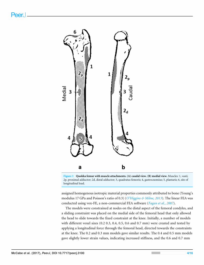
Figure 1 Quokka femur with muscle attachments. (A) caudal view. (B) medial view.Muscles: 1, vasti;2p, proximal adductor; 2d, distal adductor; 3, quadratus femoris; 4, gastrocnemius; 5, plantaris; 6, site oflongitudinal load.

assigned homogenous isotropic material properties commonly attributed to bone (Young’smodulus 17 GPa and Poisson’s ratio of 0.3) (O’Higgins & Milne, 2013). The linear FEA wasconducted using vox-FE, a non-commercial FEA software (Fagan et al., 2007).

The models were constrained at nodes on the distal aspect of the femoral condyles, anda sliding constraint was placed on the medial side of the femoral head that only allowedthe head to slide towards the fixed constraint at the knee. Initially, a number of modelswith different voxel sizes (0.2 0.3, 0.4, 0.5, 0.6 and 0.7 mm) were created and tested byapplying a longitudinal force through the femoral head, directed towards the constraintsat the knee. The 0.2 and 0.3 mm models gave similar results. The 0.4 and 0.5 mm modelsgave slightly lower strain values, indicating increased stiffness, and the 0.6 and 0.7 mm

McCabe et al. (2017), PeerJ, DOI 10.7717/peerj.3100 4/16

models were increasingly stiff. Accordingly, the 0.3 mm model was used as it gave similarresults to the 0.2 mm model, but with reduced computational time (the 0.3 mm modelscontained about 300,000 elements).

To make models of the quokka femur with different curvatures, a caudally directedload was applied to the caudal aspect of the model. After running the analysis in vox-FE,the original and new values for the 83 landmarks were analysed in the EVAN tool box(http://www.evan-society.org) together with a Stanford ply surface file representing thefemoral model. The deformation along the first principal component (PC) could then beexaggerated and the resulting femoral shape examined. In this way, coordinates representinga straight version of the quokka femur were extracted. Those new coordinates were usedin Amira to warp a surface file of the original model to the straightened state. The ‘‘scanconvert surface’’ module was used to produce an Amira mesh file which was in turn wasconverted to a new finite element mesh model. Extra-curved and reverse-curved modelswere created in the sameway, by doubling the deformation in the case of the reverse-curved,and reversing the deformation on the normal model in the case of the extra-curved model.The curvature of the resulting models, as well as a sample of eight actual quokka femora,was measured according to methods adapted from Richmond &Whalen (2001). A grid of11 evenly-spaced parallel lines was superimposed over a photo of the lateral aspect of themodels. The lines were perpendicular to the long axis of the bone, and were positioned suchthat the proximal line sat at the distal margin of the greater trochanter, and the distal linesat on the distal epiphyseal line. The intersections of these lines with the anterior marginof the model were digitised using tpsDig 2 (Rohlf, 2015). The coordinates of these pointswere translated, rotated and scaled such that the most distal landmark sat at (0,0), and themost proximal landmark sat at (1,0) on a Cartesian plane. The largest absolute y value wasused as the index of the bone’s curvature.

Forces representing the adductors and quadratus femoris (the adductor group),gastrocnemius and plantaris (gastrocnemius group), the vasti, and longitudinal forceswere applied individually and additively. In pilot analyses we used the maximum muscleforces as estimated by PCSA but these produced gross deformations of FE models that wereunrealistic and made the results unreliable. The magnitude of the forces used was 10% ofthe maximum as calculated from the PCSA. The longitudinal force was calculated as 10%of the sum forces of the biarticular muscles that cross the femur (rectus femoris and thehamstrings). This force was applied at the lateral edge of the proximal articular surface anddirected between the condyle constraints distally (Fig. 1.).

The results are presented in the form of compressive and tensile strain maps, and also byGM analysis of the deformation based on the 83 landmark coordinates after each loadingstate.

RESULTSThe data from the muscle dissections together with the calculated PCSA and estimatedmaximal forces of each muscle are provided in Table 1.

Strain contour maps for the successive addition of loads on the four models are shown inFig. 2. The first row shows that the adductor force causes caudal bending in all the models,

McCabe et al. (2017), PeerJ, DOI 10.7717/peerj.3100 5/16

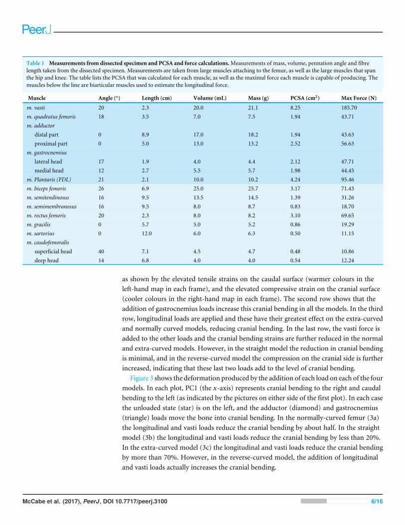
Table 1 Measurements from dissected specimen and PCSA and force calculations.Measurements of mass, volume, pennation angle and fibrelength taken from the dissected specimen. Measurements are taken from large muscles attaching to the femur, as well as the large muscles that spanthe hip and knee. The table lists the PCSA that was calculated for each muscle, as well as the maximal force each muscle is capable of producing. Themuscles below the line are biarticular muscles used to estimate the longitudinal force.

Muscle Angle (◦) Length (cm) Volume (mL) Mass (g) PCSA (cm2) Max Force (N)

m. vasti 20 2.3 20.0 21.1 8.25 185.70m. quadratus femoris 18 3.5 7.0 7.5 1.94 43.71m. adductor

distal part 0 8.9 17.0 18.2 1.94 43.63proximal part 0 5.0 13.0 13.2 2.52 56.63

m. gastrocnemiuslateral head 17 1.9 4.0 4.4 2.12 47.71medial head 12 2.7 5.5 5.7 1.98 44.45

m. Plantaris (FDL) 21 2.1 10.0 10.2 4.24 95.46m. biceps femoris 26 6.9 25.0 25.7 3.17 71.43m. semitendinosus 16 9.5 13.5 14.5 1.39 31.26m. semimembranosus 16 9.5 8.0 8.7 0.83 18.70m. rectus femoris 20 2.3 8.0 8.2 3.10 69.65m. gracilis 0 5.7 5.0 5.2 0.86 19.29m. sartorius 0 12.0 6.0 6.3 0.50 11.15m. caudofemoralis

superficial head 40 7.1 4.5 4.7 0.48 10.86deep head 14 6.8 4.0 4.0 0.54 12.24

as shown by the elevated tensile strains on the caudal surface (warmer colours in theleft-hand map in each frame), and the elevated compressive strain on the cranial surface(cooler colours in the right-hand map in each frame). The second row shows that theaddition of gastrocnemius loads increase this cranial bending in all the models. In the thirdrow, longitudinal loads are applied and these have their greatest effect on the extra-curvedand normally curved models, reducing cranial bending. In the last row, the vasti force isadded to the other loads and the cranial bending strains are further reduced in the normaland extra-curved models. However, in the straight model the reduction in cranial bendingis minimal, and in the reverse-curved model the compression on the cranial side is furtherincreased, indicating that these last two loads add to the level of cranial bending.

Figure 3 shows the deformation produced by the addition of each load on each of the fourmodels. In each plot, PC1 (the x-axis) represents cranial bending to the right and caudalbending to the left (as indicated by the pictures on either side of the first plot). In each casethe unloaded state (star) is on the left, and the adductor (diamond) and gastrocnemius(triangle) loads move the bone into cranial bending. In the normally-curved femur (3a)the longitudinal and vasti loads reduce the cranial bending by about half. In the straightmodel (3b) the longitudinal and vasti loads reduce the cranial bending by less than 20%.In the extra-curved model (3c) the longitudinal and vasti loads reduce the cranial bendingby more than 70%. However, in the reverse-curved model, the addition of longitudinaland vasti loads actually increases the cranial bending.

McCabe et al. (2017), PeerJ, DOI 10.7717/peerj.3100 6/16

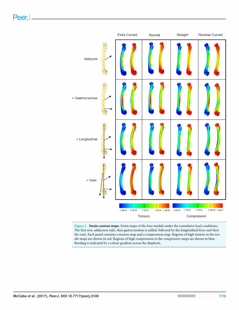
Figure 2 Strain contour maps. Strain maps of the four models under the cumulative load conditions.The first row, adductors only, then gastrocnemius is added, followed by the longitudinal force and thenthe vasti. Each panel contains a tension map and a compression map. Regions of high tension in the ten-sile maps are shown in red. Regions of high compression in the compressive maps are shown in blue.Bending is indicated by a colour gradient across the diaphysis.

McCabe et al. (2017), PeerJ, DOI 10.7717/peerj.3100 7/16

There appears to be an almost linear relationship between the model curvature and thepercentage of cranial bending mitigated by the combined action of the longitudinal andvasti loads (Fig. 4).

DISCUSSIONThis study has demonstrated that models of caudally-curved quokka femora are lessstrained than the straight or reverse-curved models. In the caudally curved models the vastiand longitudinal forces generate caudal bending—the curved bone effect—that can counterthe cranial bending due to adductor and ankle plantarflexor forces. In the straight model,the curved bone effect is too small to effectively balance the cranial bending strains. In thereverse-curved model the curved bone effect is operating to exacerbate the cranial bending.This study raises a number of issues that are further explored in this discussion. Severalhypotheses have been proposed to explain the existence of curvature in long bones, but noneaccount for the direction of curvature. The forces we applied were 10% of the maximumpossible forces based on PCSA, but there is no reason to assume that all the muscles operateat the same proportion of their potential, and it seems likely that in reality the vasti andlongitudinal forces are relatively larger than the adductor and ankle plantarflexor forces.The degree of curvature of the models seems to bear a linear relationship with the amountof bending induced by the longitudinally acting forces (curved bone effect).

The transverse forces from the adductor and gastrocnemius muscles produce cranialbending strains to a similar degree in all four models (Figs. 2 and 3). There are smalldifferences which result from the fact that, although the size and direction of the forcesare constant, the models have different curvature, and so the line of the shaft with respectto the forces and the length of the model are slightly different. However, the longitudinalforces have markedly different effects on the four models. The longitudinal forces have verylittle effect on the straight model. On the normal and extra-curved models, the longitudinalforces have caudal bending effects that increase with curvature, and on the reverse-curvedmodel the same forces have a cranial bending effect. The overall result is that in the normaland extra-curved models the longitudinal and transverse forces cause bending strains thatcancel each other out. Thus, we can say that in the case of the quokka femur, the curvaturehas a strain-reducing effect, and this supports the ideas of Pauwels (1980, Fig. 12) andFrost (1964, Figs. 5 & 7). This reinforces the theory that bone curvature is an adaptation toreduce bending strain in bones that are subjected to habitual bending loads (Milne, 2016).

Various other hypotheses have been proposed to explain the curvature seen in longbones: that curvature exists to create a strain gradient to stimulate bone remodellingfor tissue maintenance (Lanyon, 1980); that the curvature exists to provide a warningof approaching strain limits (Currey, 1984); or that the curvature makes the directionof bending strains predictable (Bertram & Biewener, 1988). These ideas all suffer fromthe same weakness: they would work equally well regardless of the direction of the curve.However, among terrestrial quadrupeds, the bones all have the same direction of curvature.The present study demonstrated that reversing the direction of curvature has the effect ofmagnifying the bending strains, which would be neither adaptive nor beneficial. Therefore,it is apparent that the direction of curvature is of biomechanical significance.

McCabe et al. (2017), PeerJ, DOI 10.7717/peerj.3100 8/16

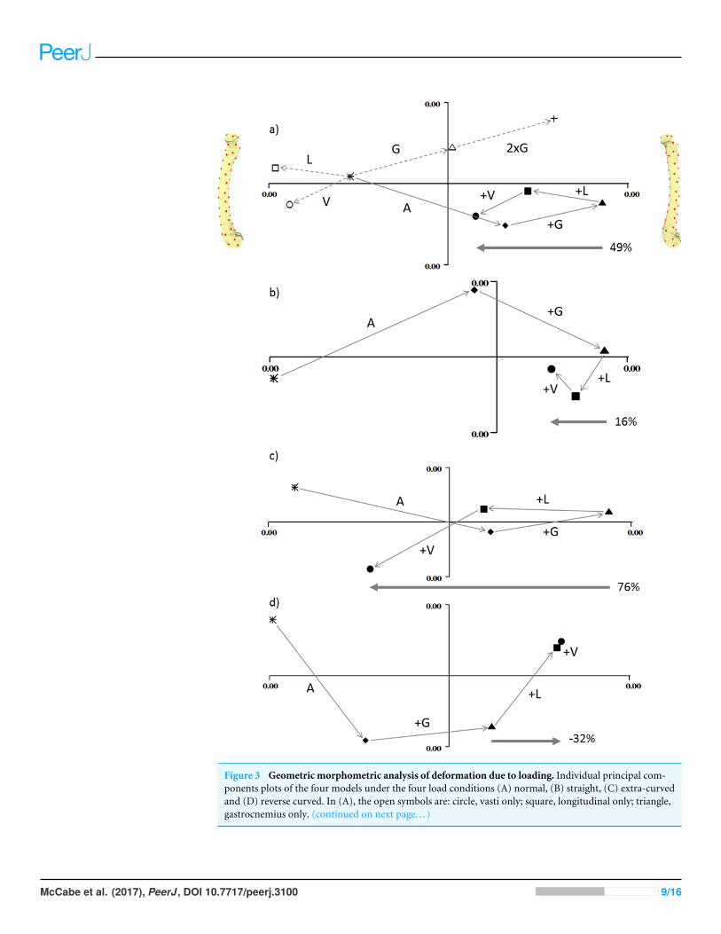
Figure 3 Geometric morphometric analysis of deformation due to loading. Individual principal com-ponents plots of the four models under the four load conditions (A) normal, (B) straight, (C) extra-curvedand (D) reverse curved. In (A), the open symbols are: circle, vasti only; square, longitudinal only; triangle,gastrocnemius only. (continued on next page. . . )

McCabe et al. (2017), PeerJ, DOI 10.7717/peerj.3100 9/16

Figure 3 (. . .continued)The cross in (A) demonstrates that doubling the gastrocnemius force magnitude doubles the vector dis-placement in shape space. In all figures, the filled symbols are: star, unloaded; diamond, adductor only;triangle, adductor and gastrocnemius; square, adductor, gastrocnemius and longitudinal; circle, adduc-tor; gastrocnemius, longitudinal and vasti. In all figures, PC1 is the x axis and PC2 is the y axis. Along thex axis, caudal bending is to the left and cranial bending is to the right, which is indicated by the models ateither end of the x axis in (A). These are visualisation aids only, not ‘‘end-points’’. In each figure the arrowand percentage indicates ‘‘the curved bone effect’’, the extent to which the longitudinal and vasti forcescan counter the cranial bending due the adductors and gastrocnemius.

Applied loads and their effect on the resultsOur results seem to indicate that the extra-curved model is less strained than the normalmodel and this raises an obvious question: why isn’t the quokka femur more curved than itis? The forces applied in themodelling performed here were based on 10% of themaximumpossible force for each muscle. For the normally-curved model, the gastrocnemius andlongitudinal forces would need to be doubled in order to completely neutralise bendingdue to the transverse forces.

It is very likely that the caudal bending forces used in this analysis were underestimated.In particular, the longitudinal force was very difficult to quantify. In life it would becomprised of components from joint reaction forces, gravity and spanning musculature.In this study only the component from the spanning musculature was accounted for, asit was the only easily-quantifiable component. While this conservative estimate of thelongitudinal force was likely the greatest source of error, it is also probable that the vastiforce was underestimated. The vasti would be expected to generate enough force to producean extension moment at the knee, not only to resist the ground reaction force, but also toresist the flexion moment caused by the gastrocnemius and hamstrings.

The actual forces that quokka femora are subject to during stance phase are notknown—indeed, no reference was found to any similar data on any marsupials or evenother mammals of similar size. PCSA was therefore chosen as a ‘‘best estimate’’ method.Faced with the same problem, Milne (2016) assigned each force vector a magnitude equalto body weight. PCSA preserves the relative force-magnitude of the muscle groups, suchthat larger groups have a correspondingly larger effect on the model. However, initialtrials soon revealed that using 100% PCSA was unviable, as it produced macroscopicdeformation in the models. So, the PCSA values were scaled to 10%, which gave forcevalues that were remarkably close to body weight, which lends considerable credibility toMilne’s methodology. This scaling of the muscle forces may appear arbitrary, however, itis of little relevance to the results. Regardless of the absolute magnitudes, if the forces arescaled in proportion to each other—which they were—the results will be the same; therelative effects of each of the muscle groups will be preserved.

PCSA-scaled muscle forces assume that all the muscles are active to the same degree atthe same time. This, although potentially unrealistic, was unavoidable. However, the PCplots contain unique vector properties that allow other force combinations to be estimatedfrom the existing data. The displacement on the PC plots caused by each muscle groupis directly proportional to the magnitude of the force. This means that by simple vector

McCabe et al. (2017), PeerJ, DOI 10.7717/peerj.3100 10/16

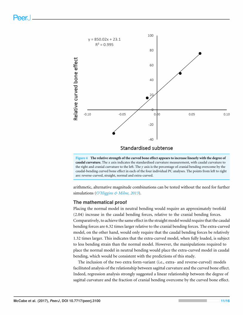
Figure 4 The relative strength of the curved bone effect appears to increase linearly with the degree ofcaudal curvature. The x axis indicates the standardised curvature measurement, with caudal curvature tothe right and cranial curvature to the left. The y axis is the percentage of cranial bending overcome by thecaudal-bending curved bone effect in each of the four individual PC analyses. The points from left to rightare: reverse-curved, straight, normal and extra-curved.

arithmetic, alternative magnitude combinations can be tested without the need for furthersimulations (O’Higgins & Milne, 2013).

The mathematical proofPlacing the normal model in neutral bending would require an approximately twofold(2.04) increase in the caudal bending forces, relative to the cranial bending forces.Comparatively, to achieve the same effect in the straightmodelwould require that the caudalbending forces are 6.32 times larger relative to the cranial bending forces. The extra-curvedmodel, on the other hand, would only require that the caudal bending forces be relatively1.32 times larger. This indicates that the extra-curved model, when fully loaded, is subjectto less bending strain than the normal model. However, the manipulations required toplace the normal model in neutral bending would place the extra-curved model in caudalbending, which would be consistent with the predictions of this study.

The inclusion of the two extra form-variant (i.e., extra- and reverse-curved) modelsfacilitated analysis of the relationship between sagittal curvature and the curved bone effect.Indeed, regression analysis strongly suggested a linear relationship between the degree ofsagittal curvature and the fraction of cranial bending overcome by the curved bone effect.

McCabe et al. (2017), PeerJ, DOI 10.7717/peerj.3100 11/16

This linear regression analysis contained only four data points, so it would be premature tocite this data as conclusive. There does appear to be a strong trend, although interpolationof further data points would be required to determine the mathematical nature of therelationship present.

Intuitively, the curvature moment arm (subtense) is the mechanical purchase on which alongitudinal load acts. Therefore, the positive relationship found in Fig. 4 is not unexpected.The only remaining question is: is this relationship linear? Swartz (1990) observed thatthe expected cortical bending stress is directly proportional to the curvature moment arm(subtense). While this strongly suggests a linear relationship between bending momentmagnitude and initial curvature, it does not completely describe the observed trend inFig. 4. However, it is possible to demonstrate mathematically that the observed trend isindeed linear.

The femur can be modelled mathematically as an idealised curved beam with a hollowcylindrical cross section (note that the following analyses are adapted from Case, Chilver& Ross, 1999) (see Fig. 5). All four femoral models are assumed to have the same chordlength (L), longitudinal load magnitude (P), material properties (E = Young’s modulus),and diameter (I = cross-sectional area moment of inertia). Straight beams, when loadedaxially, will buckle under a critical load (Euler load, Pe , Eq. 1). At this point, the bendingmoment at an arbitrary distance (x) along the chord is the product of the longitudinalload and the induced curvature (v, Eq. 2). If the beam has an initial curvature (v0), thenthe bending moment is the product of the longitudinal load and the total curvature at thatpoint (Eq. 3). If the beam is initially unloaded, then the bending moment at an arbitrarydistance (x) along the chord is proportional to the change in curvature at that point (Eq.4). Solving this differential equation yields Eq. 5. It is assumed for simplicity that the initialcurvature can be modelled by a half a sine curve of amplitude a (Eq. 6). The resistance of abeam to bending (k) is described in Eq. 7. This equation, as well as Eq. 6 can be substitutedinto Eq. 5. This yields Eq. 8.

The greatest bending moment will be experienced when the curvature moment arm ismaximised. This, by definition, is the subtense. So, substituting the subtense into Eq. 8gives an expression for the expected increase in curvature at the point of maximum initialcurvature (Eq. 9). This expression can be substituted into Eq. 3, to give an expression forthe bending moment experienced at the point of maximum curvature (Eq. 10). Therefore,this is the maximum bending moment. This equation can be rearranged to give anexpression for the maximum bending moment as a function of the subtense (Eq. 11). Thelongitudinal load and Euler load are consistent between the four models, which means thatthe expression that is the coefficient of a in Eq. 11 is a constant. Thus, the magnitude ofthe bending moment induced by longitudinal loading is directly proportional to the initialcurvature (subtense).

M expresses the bendingmoment induced by the curved bone effect.T can be introducedto express the bending moment caused by the habitual loading; this was effectively constantbetween the four models. In all four models, M was only able to overcome a fraction ofT ; this fraction can be expressed as z, according to Eq. 12. Equation 11 can be substitutedinto Eq. 12, and then rearranged to find an expression for z in terms of a (Eq. 13). The

McCabe et al. (2017), PeerJ, DOI 10.7717/peerj.3100 12/16

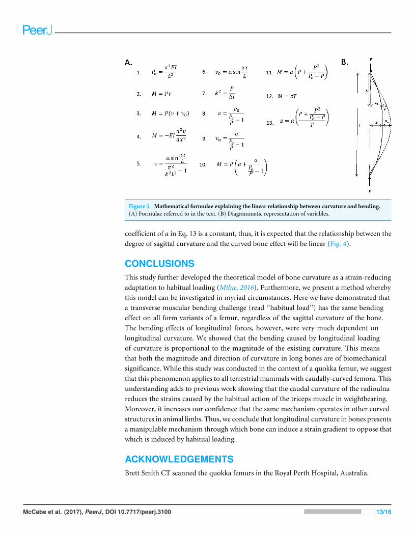
Figure 5 Mathematical formulae explaining the linear relationship between curvature and bending.(A) Formulae referred to in the text. (B) Diagrammatic representation of variables.

coefficient of a in Eq. 13 is a constant, thus, it is expected that the relationship between thedegree of sagittal curvature and the curved bone effect will be linear (Fig. 4).

CONCLUSIONSThis study further developed the theoretical model of bone curvature as a strain-reducingadaptation to habitual loading (Milne, 2016). Furthermore, we present a method wherebythis model can be investigated in myriad circumstances. Here we have demonstrated thata transverse muscular bending challenge (read ‘‘habitual load’’) has the same bendingeffect on all form variants of a femur, regardless of the sagittal curvature of the bone.The bending effects of longitudinal forces, however, were very much dependent onlongitudinal curvature. We showed that the bending caused by longitudinal loadingof curvature is proportional to the magnitude of the existing curvature. This meansthat both the magnitude and direction of curvature in long bones are of biomechanicalsignificance. While this study was conducted in the context of a quokka femur, we suggestthat this phenomenon applies to all terrestrial mammals with caudally-curved femora. Thisunderstanding adds to previous work showing that the caudal curvature of the radioulnareduces the strains caused by the habitual action of the triceps muscle in weightbearing.Moreover, it increases our confidence that the same mechanism operates in other curvedstructures in animal limbs. Thus, we conclude that longitudinal curvature in bones presentsa manipulable mechanism through which bone can induce a strain gradient to oppose thatwhich is induced by habitual loading.

ACKNOWLEDGEMENTSBrett Smith CT scanned the quokka femurs in the Royal Perth Hospital, Australia.

McCabe et al. (2017), PeerJ, DOI 10.7717/peerj.3100 13/16

ADDITIONAL INFORMATION AND DECLARATIONS

FundingVox-FE was developed by Michael Fagan, Roger Phillips and Paul O’Higgins with supportfrom BBSRC (BB/E013805; BB/E009204). The funders had no role in study design, datacollection and analysis, decision to publish, or preparation of the manuscript.

Competing InterestsThe authors declare there are no competing interests.

Author Contributions• Kyle McCabe conceived and designed the experiments, performed the experiments,analyzed the data, wrote the paper, prepared figures and/or tables, reviewed drafts of thepaper.• Keith Henderson and Jess Pantinople conceived and designed the experiments, analyzedthe data, reviewed drafts of the paper.• Hazel L. Richards wrote the paper, prepared figures and/or tables, reviewed drafts of thepaper.• Nick Milne conceived and designed the experiments, performed the experiments,analyzed the data, contributed reagents/materials/analysis tools, wrote the paper,prepared figures and/or tables, reviewed drafts of the paper.

Data AvailabilityThe following information was supplied regarding data availability:

The raw data has been supplied as a Supplemental Information 1.

Supplemental InformationSupplemental information for this article can be found online at http://dx.doi.org/10.7717/peerj.3100#supplemental-information.

REFERENCESAnapol F, Barry K. 1996. Fiber architecture of the extensors of the hindlimb in

semiterrestrial and arboreal guenons. American Journal of Physical Anthropology99(3):429–447DOI 10.1002/(SICI)1096-8644(199603)99:3<429::AID-AJPA5>3.0.CO;2-R.

Bertram J, Biewener A. 1988. Bone curvature: sacrificing strength for load predictability?Journal of Theoretical Biology 131:75–92 DOI 10.1016/S0022-5193(88)80122-X.

Biewener AA, Thomason J, Goodship A, Lanyon LE. 1983. Bone stress in the horse fore-limb during locomotion at different gaits: a comparison of two experimental meth-ods. Journal of Biomechanics 16(8):565–576 DOI 10.1016/0021-9290(83)90107-0.

McCabe et al. (2017), PeerJ, DOI 10.7717/peerj.3100 14/16

Case J, Chilver L, Ross CT. 1999. Strength of materials and structures. 4th edition.Oxford: Butterworth-Heinemann.

Copploe JV, Blob RW, Parrish JHA, Butcher MT. 2015. In vivo strains in the femurof the nine-banded armadillo (Dasypus novemcinctus). Journal of Morphology276:889–899 DOI 10.1002/jmor.20387.

Currey JD. 1984. Can strains give adequate information for adaptive bone remodelling?Calcification Tissue International 36:A118–S122 DOI 10.1007/BF02406144.

Elftman HO. 1929. Functional adaptations of the pelvis in marsupials. Bulletin of theAMNH 58: Article 5.

FaganMJ, Curtis N, Dobson CA, Karunanayake JH, Kitpczik K, MoazenM, Page L,Phillips R, O’Higgins P. 2007. Voxel-based finite analysis—working directly withmicroCT scan data [Abstract]. Journal of Morphology 268:1071.

Freedman L, Twomey LT. 1979. Relative growth rates of limb muscles in the diprotodontmarsupial, Setonix brachyurus. Journal of Zoology 188(2):161–171.

Frost HM. 1964. Laws of bone structure. Springfield: Charles C Thomas.Fukunaga T, Roy RR, Shellock FG, Hodgson JA, Edgerton VR. 1996. Specific tension of

human plantar flexors and dorsiflexors. Journal of Applied Physiology 80(1):158–165.Jade S, Tamvada KH, Strait DS, Grosse IR. 2014. Finite element analysis of a femur to

deconstruct the paradox of bone curvature. Journal of Theoretical Biology 341:53–63DOI 10.1016/j.jtbi.2013.09.012.

Lanyon L. 1980. The influence of function on the development of bone curvature. Anexperimental study on the rat tibia. Journal of Zoology 192:457–466DOI 10.1111/j.1469-7998.1980.tb04243.x.

Lanyon LE, Baggott DG. 1976.Mechanical function as an influence on the structure andform of bone. Bone & Joint Journal 58-B(4):436–443.

Lanyon LE, Bourn S. 1979. The influence of mechanical function on the developmentand remodeling of the tibia. An experimental study in sheep. The Journal of Bone andJoint Surgery 61(2):263–273 DOI 10.2106/00004623-197961020-00019.

Lanyon LE, Magee PT, Baggott DG. 1979. The relationship of functional stress and strainto the processes of bone remodelling. An experimental study on the sheep radius.Journal of Biomechanics 12(8):593–600 DOI 10.1016/0021-9290(79)90079-4.

McGowan CP, Skinner J, Biewener AA. 2008.Hind limb scaling of kangaroos andwallabies (superfamily Macropodoidea): implications for hopping performance,safety factor and elastic savings. Journal of Anatomy 212(2):153–163DOI 10.1111/j.1469-7580.2007.00841.x.

Milne N. 2016. Curved bones: an adaptation to habitual loading. Journal of TheoreticalBiology 407:18–24 DOI 10.1016/j.jtbi.2016.07.019.

O’Higgins P, Milne N. 2013. Applying geometric morphometrics to compare changes insize and shape arising from finite elements analyses. Hystrix 24:126–132DOI 10.4404/hystrix-24.1-6284.

Pauwels F. 1980. Biomechanics of the locomotor apparatus. Translation of the Germanedition 1965. Berlin: Springer-Verlag.

McCabe et al. (2017), PeerJ, DOI 10.7717/peerj.3100 15/16

Powell PL, Roy RR, Kanim P, Bello MA, Edgerton VR. 1984. Predictability of skeletalmuscle tension from architectural determinations in guinea pig hindlimbs. Journal ofApplied Physiology 57(6):1715–1721.

Richmond B,WhalenM. 2001. De Bonis L, Koufos G, Andrews P, eds. Forelimb function,bone curvature and phylogeny of sivapithecus, in hominoid evolution and climaticchange in Europe. Vol. 2. Cambridge: Cambridge University Press, 326–348.

Rohlf F. 2015. TpsDig in morphometric software. New York: Stony Brook Morphometrics,Stony Brook.

Sacks RD, Roy RR. 1982. Architecture of the hind limb muscles of cats: functionalsignificance. Journal of Morphology 173(2):185–195 DOI 10.1002/jmor.1051730206.

Swartz SM. 1990. Curvature of the forelimb bones of anthropoid primates: overallallometric patterns and specializations in suspensory species. American Journal ofPhysical Anthropology 83:477–498 DOI 10.1002/ajpa.1330830409.

Swartz SM, Bertram JEA, Biewener AA. 1989. Telemetered in vivo strain analysis oflocomotor mechanics of brachiating gibbons. Nature 342(6247):270–272DOI 10.1038/342270a0.

McCabe et al. (2017), PeerJ, DOI 10.7717/peerj.3100 16/16