Embed Size (px)
Citation preview
Curve
2017-11-08
Glenn Grefer
Field Application Engineer
22017-11-08Carl Zeiss IMT, Glenn Grefer
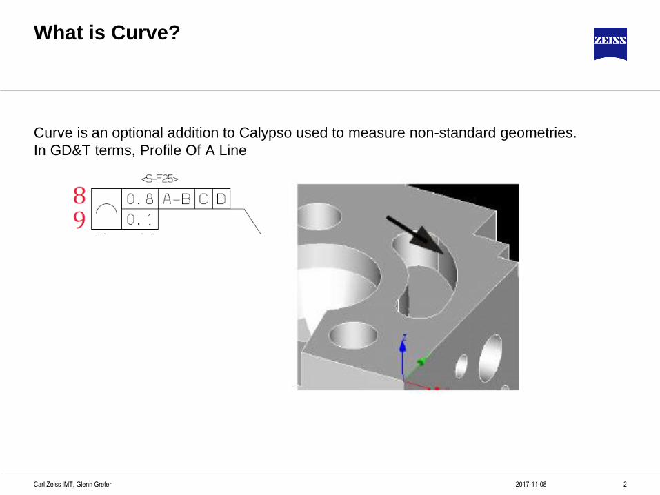
What is Curve?
Curve is an optional addition to Calypso used to measure non-standard geometries.
In GD&T terms, Profile Of A Line
32017-11-08Carl Zeiss IMT, Glenn Grefer
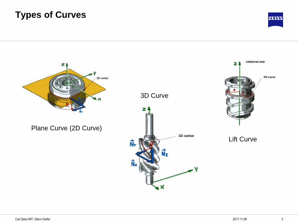
Types of Curves
Plane Curve (2D Curve)
3D Curve
Lift Curve
42017-11-08Carl Zeiss IMT, Glenn Grefer
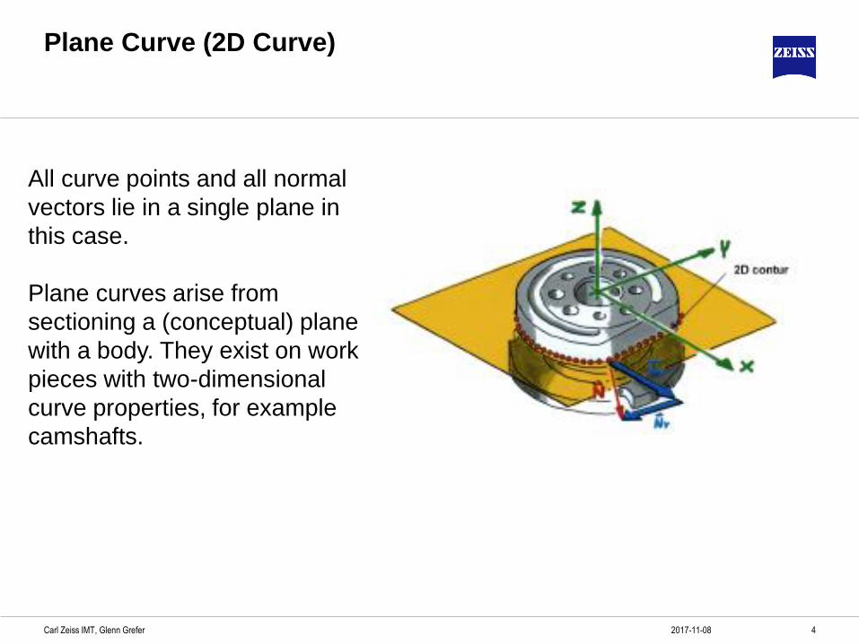
Plane Curve (2D Curve)
All curve points and all normal
vectors lie in a single plane in
this case.
Plane curves arise from
sectioning a (conceptual) plane
with a body. They exist on work
pieces with two-dimensional
curve properties, for example
camshafts.
52017-11-08Carl Zeiss IMT, Glenn Grefer
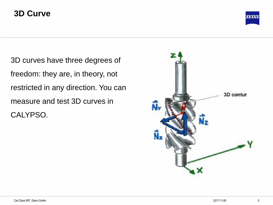
3D Curve
3D curves have three degrees of
freedom: they are, in theory, not
restricted in any direction. You can
measure and test 3D curves in
CALYPSO.
62017-11-08Carl Zeiss IMT, Glenn Grefer
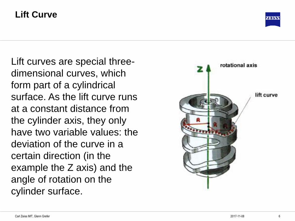
Lift Curve
Lift curves are special three-
dimensional curves, which
form part of a cylindrical
surface. As the lift curve runs
at a constant distance from
the cylinder axis, they only
have two variable values: the
deviation of the curve in a
certain direction (in the
example the Z axis) and the
angle of rotation on the
cylinder surface.
72017-11-08Carl Zeiss IMT, Glenn Grefer
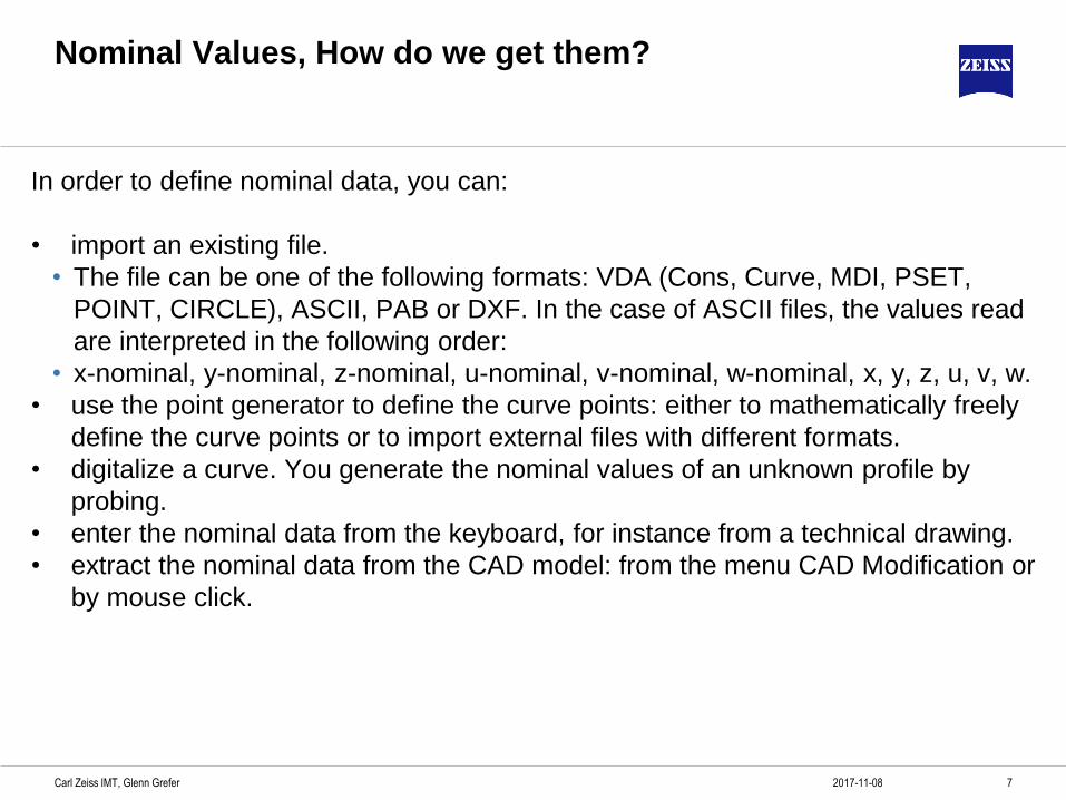
Nominal Values, How do we get them?
In order to define nominal data, you can:
• import an existing file.
• The file can be one of the following formats: VDA (Cons, Curve, MDI, PSET,
POINT, CIRCLE), ASCII, PAB or DXF. In the case of ASCII files, the values read
are interpreted in the following order:
• x-nominal, y-nominal, z-nominal, u-nominal, v-nominal, w-nominal, x, y, z, u, v, w.
• use the point generator to define the curve points: either to mathematically freely
define the curve points or to import external files with different formats.
• digitalize a curve. You generate the nominal values of an unknown profile by
probing.
• enter the nominal data from the keyboard, for instance from a technical drawing.
• extract the nominal data from the CAD model: from the menu CAD Modification or
by mouse click.
82017-11-08Carl Zeiss IMT, Glenn Grefer
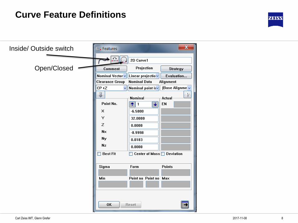
Curve Feature Definitions
Inside/ Outside switch
Open/Closed
92017-11-08Carl Zeiss IMT, Glenn Grefer
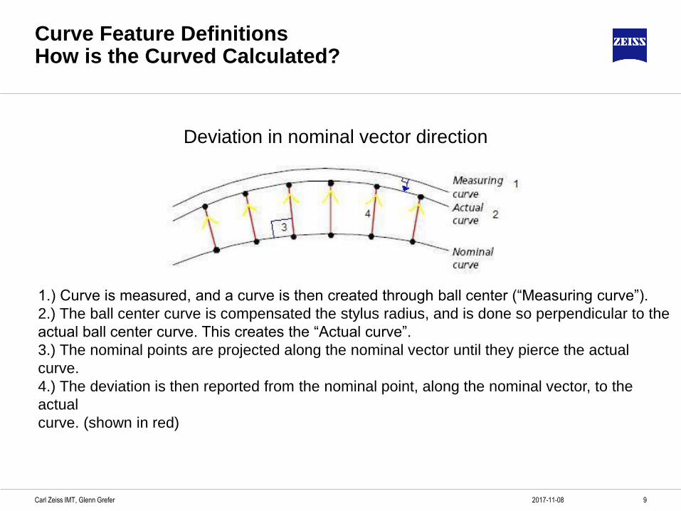
Curve Feature Definitions How is the Curved Calculated?
Deviation in nominal vector direction
1.) Curve is measured, and a curve is then created through ball center (“Measuring curve”).
2.) The ball center curve is compensated the stylus radius, and is done so perpendicular to the
actual ball center curve. This creates the “Actual curve”.
3.) The nominal points are projected along the nominal vector until they pierce the actual
curve.
4.) The deviation is then reported from the nominal point, along the nominal vector, to the
actual
curve. (shown in red)
102017-11-08Carl Zeiss IMT, Glenn Grefer
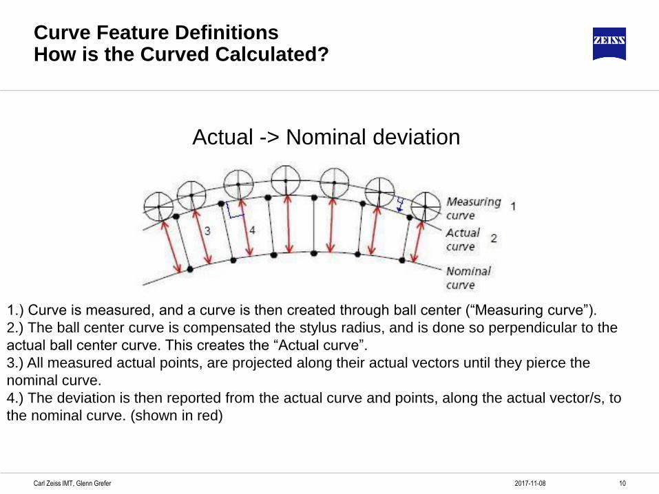
Curve Feature Definitions How is the Curved Calculated?
Actual -> Nominal deviation
1.) Curve is measured, and a curve is then created through ball center (“Measuring curve”).
2.) The ball center curve is compensated the stylus radius, and is done so perpendicular to the
actual ball center curve. This creates the “Actual curve”.
3.) All measured actual points, are projected along their actual vectors until they pierce the
nominal curve.
4.) The deviation is then reported from the actual curve and points, along the actual vector/s, to
the nominal curve. (shown in red)
112017-11-08Carl Zeiss IMT, Glenn Grefer
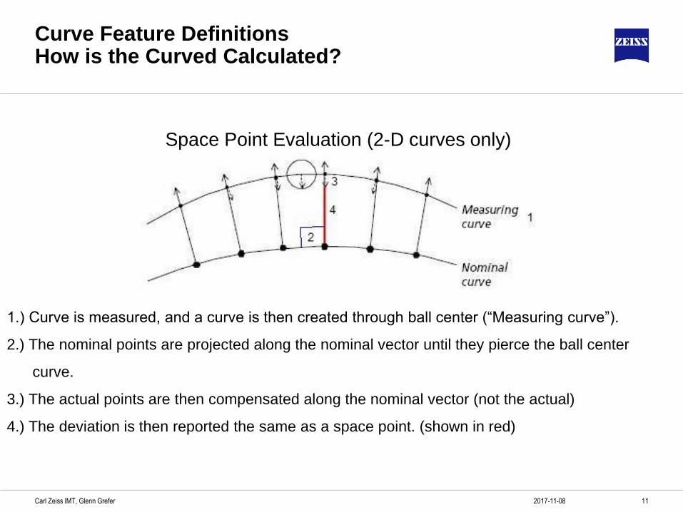
Curve Feature Definitions How is the Curved Calculated?
Space Point Evaluation (2-D curves only)
1.) Curve is measured, and a curve is then created through ball center (“Measuring curve”).
2.) The nominal points are projected along the nominal vector until they pierce the ball center
curve.
3.) The actual points are then compensated along the nominal vector (not the actual)
4.) The deviation is then reported the same as a space point. (shown in red)
122017-11-08Carl Zeiss IMT, Glenn Grefer
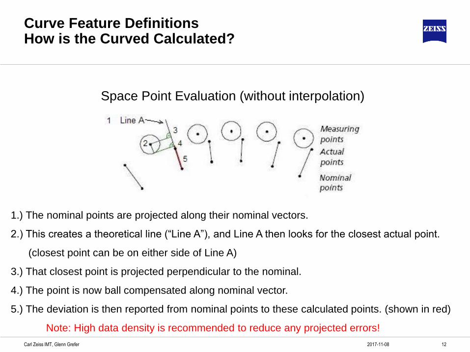
Curve Feature Definitions How is the Curved Calculated?
Space Point Evaluation (without interpolation)
1.) The nominal points are projected along their nominal vectors.
2.) This creates a theoretical line (“Line A”), and Line A then looks for the closest actual point.
(closest point can be on either side of Line A)
3.) That closest point is projected perpendicular to the nominal.
4.) The point is now ball compensated along nominal vector.
5.) The deviation is then reported from nominal points to these calculated points. (shown in red)
Note: High data density is recommended to reduce any projected errors!
132017-11-08Carl Zeiss IMT, Glenn Grefer
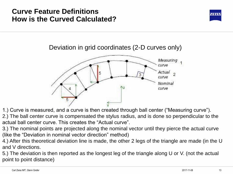
Curve Feature Definitions How is the Curved Calculated?
Deviation in grid coordinates (2-D curves only)
1.) Curve is measured, and a curve is then created through ball center (“Measuring curve”).
2.) The ball center curve is compensated the stylus radius, and is done so perpendicular to the
actual ball center curve. This creates the “Actual curve”.
3.) The nominal points are projected along the nominal vector until they pierce the actual curve
(like the “Deviation in nominal vector direction” method)
4.) After this theoretical deviation line is made, the other 2 legs of the triangle are made (in the U
and V directions.
5.) The deviation is then reported as the longest leg of the triangle along U or V. (not the actual
point to point distance)
142017-11-08Carl Zeiss IMT, Glenn Grefer
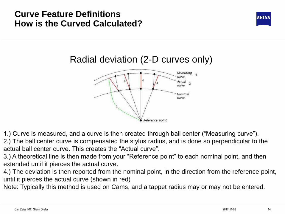
Curve Feature Definitions How is the Curved Calculated?
Radial deviation (2-D curves only)
1.) Curve is measured, and a curve is then created through ball center (“Measuring curve”).
2.) The ball center curve is compensated the stylus radius, and is done so perpendicular to the
actual ball center curve. This creates the “Actual curve”.
3.) A theoretical line is then made from your “Reference point” to each nominal point, and then
extended until it pierces the actual curve.
4.) The deviation is then reported from the nominal point, in the direction from the reference point,
until it pierces the actual curve (shown in red)
Note: Typically this method is used on Cams, and a tappet radius may or may not be entered.
152017-11-08Carl Zeiss IMT, Glenn Grefer
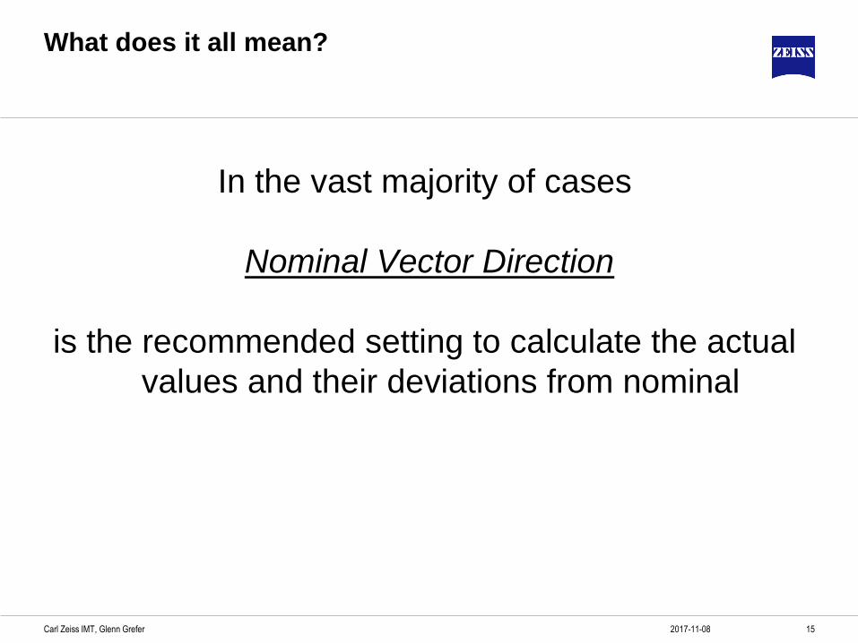
What does it all mean?
In the vast majority of cases
Nominal Vector Direction
is the recommended setting to calculate the actual
values and their deviations from nominal
162017-11-08Carl Zeiss IMT, Glenn Grefer
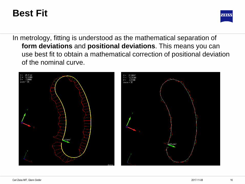
Best Fit
In metrology, fitting is understood as the mathematical separation of
form deviations and positional deviations. This means you can
use best fit to obtain a mathematical correction of positional deviation
of the nominal curve.
172017-11-08Carl Zeiss IMT, Glenn Grefer
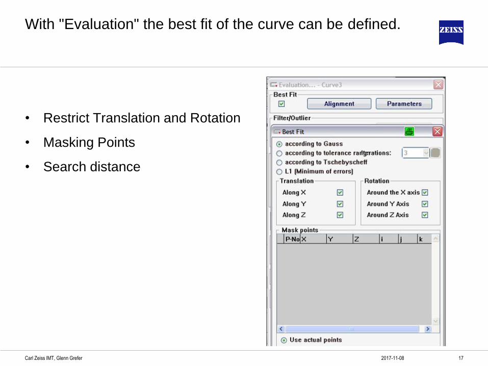
With "Evaluation" the best fit of the curve can be defined.
• Restrict Translation and Rotation
• Masking Points
• Search distance
182017-11-08Carl Zeiss IMT, Glenn Grefer
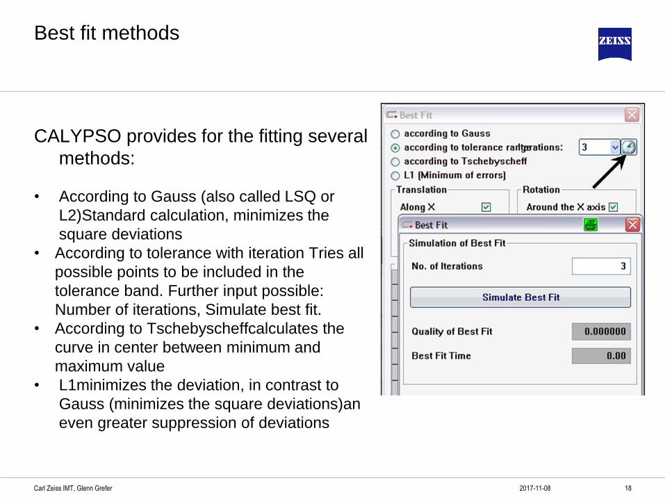
Best fit methods
CALYPSO provides for the fitting several
methods:
• According to Gauss (also called LSQ or
L2)Standard calculation, minimizes the
square deviations
• According to tolerance with iteration Tries all
possible points to be included in the
tolerance band. Further input possible:
Number of iterations, Simulate best fit.
• According to Tschebyscheffcalculates the
curve in center between minimum and
maximum value
• L1minimizes the deviation, in contrast to
Gauss (minimizes the square deviations)an
even greater suppression of deviations
192017-11-08Carl Zeiss IMT, Glenn Grefer
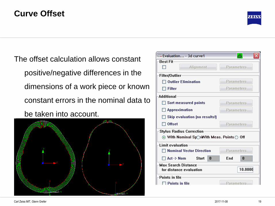
Curve Offset
The offset calculation allows constant
positive/negative differences in the
dimensions of a work piece or known
constant errors in the nominal data to
be taken into account.
202017-11-08Carl Zeiss IMT, Glenn Grefer
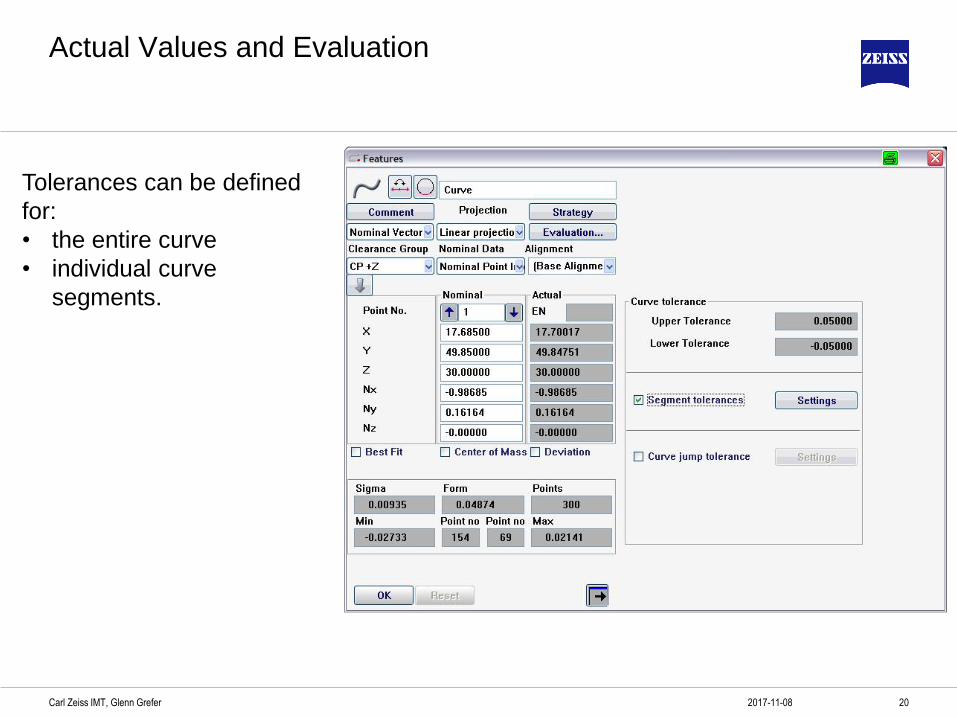
Actual Values and Evaluation
Tolerances can be defined
for:
• the entire curve
• individual curve
segments.
212017-11-08Carl Zeiss IMT, Glenn Grefer
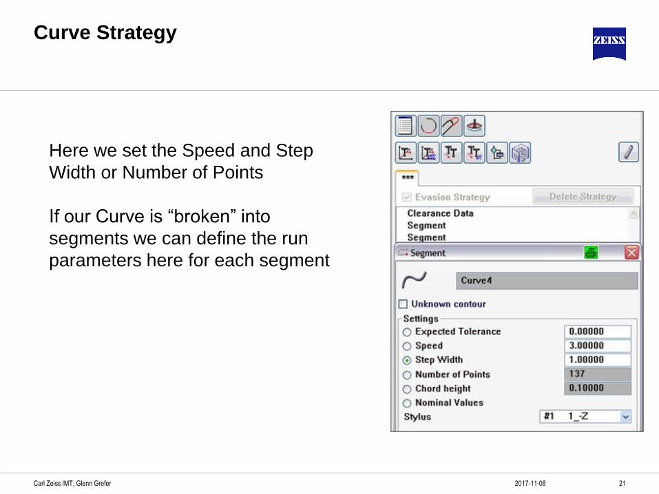
Curve Strategy
Here we set the Speed and Step
Width or Number of Points
If our Curve is “broken” into
segments we can define the run
parameters here for each segment

222017-11-08Carl Zeiss IMT, Glenn Grefer