Curves and Surfaces (cont’)

Amy Zhang

Conversion between Representations

Example: Convert a curve from a cubic B-spline curve to the Bézier form:

From Curve to Surface Recall that a parametrically defined curve in 3D is

given by three univariate functions:

where 0 ≤u≤1 By varying u from 0 to 1, a curve is swept out in 3D Similarly, a parametric surface is defined by three

bivariate functions:

where 0 ≤u≤1 and 0 ≤v≤1 By varying u from 0 to 1while keeping v constant, a

curve is swept out in 3D An infinity of such curves exists as v is varied from 0 to

1, and this defines a surface in 3D

Parametric Surfaces A single surface element, also known as a

patch, is the surface traced out as the parameters (u,v) take all values between 0 and 1

Complex surfaces are modelled using nets of individual patches analogous to the way in which complex curves are made up of individual curve segments

The teapot is made up of32 Bézier patches

Like in the case of curves, cubic basis functions, which are a good compromise between complexity and flexibility, are most commonly used in compute graphics

Bicubic parametric patches are defined over a rectangular domain in u,v-space and the boundary curves of the patch are themselves cubic polynomial curves

Parametric Surfaces Advantages of patch representation over

polygon mesh representation: Conciseness: A parametric representation of a

surface is “exact” and “economic”, and mass properties, like surface area and volume, are extractable from such a description

Parametric Surfaces Deformation and shape change:

Deformation of a parametric surface can be achieved by moving the control points that define it. The deformations will appear just as smooth and accurately represented as the un-deformed counterpart when rendered

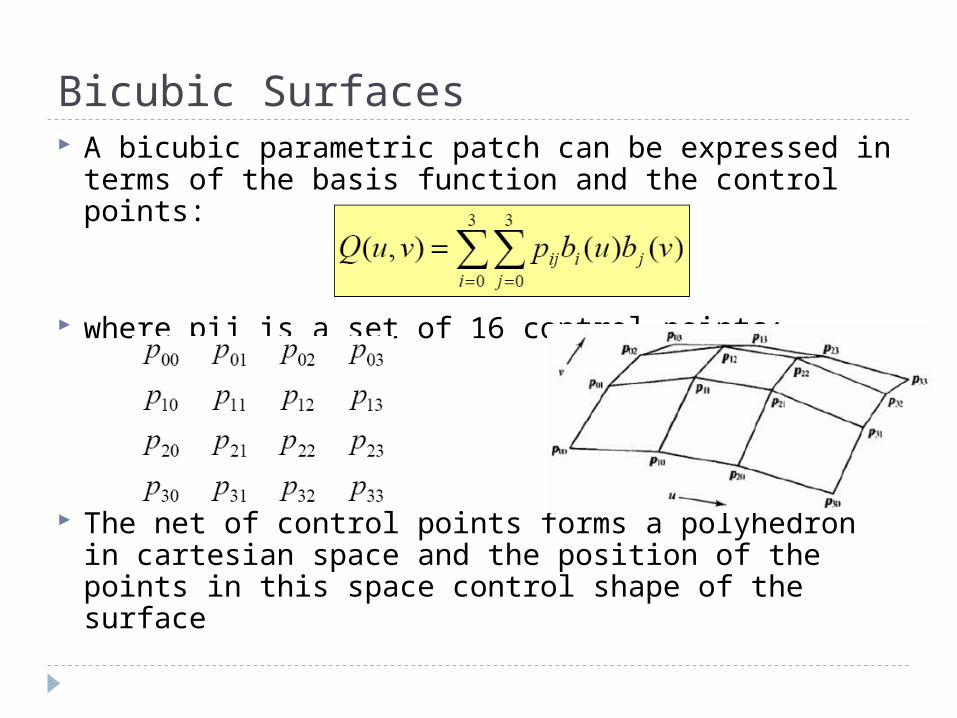
Bicubic Surfaces A bicubic parametric patch can be expressed in

terms of the basis function and the control points:

where pij is a set of 16 control points:

The net of control points forms a polyhedron in cartesian space and the position of the points in this space control shape of the surface

Bicubic Surfaces Example: The effect of lifting one of the

control point of a Bézier patch

Bicubic Surfaces Matrix formulation:

where

The matrix M is the characteristic matrix of the particular form e.g.,MB for Bézier patch and MBS for B-spline patch

The matrix P is a 4×4 matrix that contains the 16 control points

Bézier Patch A Bézier patch is defined in matrix notion by:

and alternatively by:

Note that the boundary curves of a Bézier patch are themselves Bézier curves, e.g.,

The Bézier patch hasanalogous properties to and advantages of the Bézier curve

Bézier Patch Differentiation:

Bézier Patch Differentiation at the corners:

Bézier Patch Joining 2 Bézier patches

Q and R with control points qij and rij Zero order continuity:

q3i= r0i for i =0,…,3 First order continuity:

(q3i–q2i) =k(r1i–r0i)for i =0,…,3

The above constraints may be too severe:

Any corner point cannotbe moved withoutcontrolling 8 adjacentpoints to maintaincontinuity

Bézier Patch Recall that a Bézier curve can be rendered

efficiently by recursive subdivision

Bézier Patch Similarly, a Bézier Patch can be rendered by

successively subdividing the control polygons into a series of polygons that represent the Bézier surface to a given tolerance in curvature.

The process of recursive subdivision of a Bézier Patch is called patch splitting.

The result polygons from patch splitting can be passed to a conventional polygon render and standard rendering techniques can be used to render surfaces made up of nets of patches.

Bézier Patch Due to the orthogonality of the parametric

directions u& v, a Bézier patch can be split in one parameter without considering the other

Bézier Patch Consider a patch to be made up of 4

curves, the control points of which correspond to the rows / columns of P

Splitting is then applied to these curves separately, yielding 2 sets of 4 curves qij& rij

These 2 sets of 4 curves then give 2 subpatches of the original patch

Bézier Patch A given patch is subdivided down until the

convex hull is deem to be sufficiently planar and the edges are sufficiently linear: Flatness is tested by forming a plane

between 3 corner control points and measuring how far the remaining control points deviate from this plane

Linearity of the edges is tested by measuring how far the interior control points of the edge deviate from the line joining the end control points

Bézier Patch The patch is then turned into 2 triangles by

taking the 4 corners of the patch as the triangle vertices

The surface normal at each corner is then computed as the cross product of the 2 tangent vectors at the corner, e.g.,

Bézier Patch The cracking problem will appear due to the

independent subdivision of adjacent subpatches:

Uniform B-spline Patch A uniform B-splinepatch is defined in matrix

notion by:

A composite B-spline surface is C2 continuous across the patches

The B-spline patch has analogous properties to and advantages of the B-spline curve

Converting a B-spline patch to a Bézier patch for rendering: