FEDERAL RESERVE BANK OF SAN FRANCISCO

WORKING PAPER SERIES

Cyclical and Market Determinants of Involuntary Part-Time Employment

Robert G. Valletta Federal Reserve Bank of San Francisco

Leila Bengali

Yale University

Catherine van der List University of British Columbia

March 2018

Working Paper 2015-19

http://www.frbsf.org/economic-research/publications/working-papers/2015/19/

Suggested citation:

Valletta, Robert G, Leila Bengali, Catherine van der List. 2018. “Cyclical and Market Determinants of Involuntary Part-Time Employment.” Federal Reserve Bank of San Francisco Working Paper 2015-19. https://doi.org/10.24148/wp2015-19 The views in this paper are solely the responsibility of the authors and should not be interpreted as reflecting the views of the Federal Reserve Bank of San Francisco or the Board of Governors of the Federal Reserve System.

Cyclical and Market Determinants of Involuntary Part-Time Employment

Robert G. Valletta* Federal Reserve Bank of San Francisco

101 Market Street San Francisco, CA 94105

(415) 974-3345 rob.valletta@sf.frb.org

Leila Bengali

Yale University leila.bengali@yale.edu

Catherine van der List

University of British Columbia catherine.vanderlist@alumni.ubc.ca

First version: December 2, 2015 Revised: January 2018

Minor edits: March 2018 Keywords: part-time employment, business cycle, supply and demand JEL classification: J22, J23 *Corresponding author. The authors thank FRBSF colleagues, Bob Triest, other Federal Reserve staff, and seminar participants at the University of Wisconsin IRP Summer workshop and the University of Illinois at Urbana-Champaign (School of Labor and Employment Relations) for their comments at various stages of this research. They also thank the editor at Journal of Labor Economics, Paul Oyer, and two anonymous referees for their comments and guidance. Nathaniel Barlow provided helpful research assistance. The views expressed in this paper are solely those of the authors and are not attributable to the Federal Reserve Bank of San Francisco or the Federal Reserve System.

Cyclical and Market Determinants of Involuntary Part-Time Employment

Abstract The fraction of the U.S. workforce identified as involuntary part-time workers rose to new highs during the U.S. Great Recession and came down only slowly in its aftermath. We assess the determinants of involuntary part-time work using an empirical framework that accounts for business cycle effects and persistent structural features of the labor market. We conduct regression analyses using state-level panel and individual data for the years 2003-2016. The results indicate that the persistent market-level factors, most notably shifting industry composition, can largely explain sustained elevation in the incidence of involuntary part-time work since the recession.

2

Cyclical and Market Determinants of Involuntary Part-Time Employment

I. Introduction

Part-time employment is common in the United States. Since the mid-1990s, on average

slightly more than one in six U.S. civilian employees worked part-time hours, defined as fewer

than 35 hours per week. In their tracking of part-time employment, the U.S. Bureau of Labor

Statistics (BLS) distinguishes between individuals who work part time voluntarily (“non-

economic reasons”) and those who work part time involuntarily (“economic reasons”). Although

the voluntary part-time group is much larger, interest in the involuntary part-time group has

increased in recent years as its share of the workforce reached unusually high levels during the

Great Recession of 2007-2009. Moreover, as the U.S. economy recovered from that recession,

the level of involuntary part-time work remained relatively high.

Some policymakers and analysts have raised the possibility that the persistent elevated

level of involuntary part-time work in the United States represents labor underutilization, or

labor market “slack,” beyond that reflected in the unemployment rate (e.g., Yellen 2014;

Blanchflower and Levin 2015). This interpretation has been raised for other countries as well

(e.g., Bell and Blanchflower 2014; IMF 2017) Alternatively, elevated involuntary part-time

employment may reflect labor market changes that are independent of the business cycle and

hence persistent, such as the ongoing shift to a service-based economy and the growth of the on-

demand or “gig” economy (Golden 2016; Bracha and Burke 2017).

In this paper, we examine the determinants of involuntary part-time work, distinguishing

between variation associated with the aggregate business cycle and variation attributable to more

persistent structural features of the labor market. Existing research on the characteristics and

3

behavior of involuntary part-time workers is relatively limited in quantity and scope. A small

literature from the 1980s and 1990s focused on identifying the behavioral distinction between

voluntary and involuntary part-time work and provided information on a limited set of

explanatory factors (Stratton 1996; Leppel and Clain 1988, 1993; Fallick 1999; Tilly 1991). A

number of recent studies provided descriptive analyses of involuntary part-time work and

examined the potential impact of the Affordable Care Act’s requirement that large employers

provide health insurance to full-time workers (e.g., Cajner, Mawhirter, Nekarda, and Ratner

2014; Canon, Kudlyak, Luo, and Reed 2014; Robertson and Terry 2014; Golden 2016; Even and

Macpherson 2017; Dillender, Heinrichs, and Houseman 2016; Garrett, Kaestner, and

Gangopadhyaya, 2017; Mathur, Slavova, and Strain 2016; Moriya, Selden, and Simon 2016).

Borowczyk-Martins & Lalé (2016, 2017) used data on flows between labor market states to

illustrate the rising importance of transitions between full-time and involuntary part-time jobs

over business cycles and also over the longer term in the United States and the United Kingdom.

We expand on existing research by developing a general empirical framework for

understanding changes in the incidence of involuntary part-time work and assessing the

quantitative impact of key explanatory factors for the years 2003 through 2016. As we show

below, changes in aggregate workforce composition do not make a meaningful direct

contribution to changes in the level of involuntary part-time work over our sample frame. We

therefore rely on state-level panel data for our primary empirical analyses. Importantly, this

framework enables us to jointly model and hence properly distinguish between changes in

cyclical labor market conditions at the state level and changes in structural features of state labor

markets and the composition of their workforces. The structural features include demand and

supply determinants of involuntary part-time work, in particular industry employment shares,

4

labor costs, and workforce demographics. Unlike a conventional composition adjustment, which

accounts only for changes occurring within groups, our regression framework identifies the

overall effects of changing workforce composition based on underlying shifts in demand and

supply for part-time work. The cyclical and structural market factors that we identify can largely

account for the aggregate changes in involuntary part-time work observed during the Great

Recession of 2007-2009 and its aftermath.

Our analysis proceeds as follows. We begin in Section II by defining the relevant

concepts and patterns regarding part-time employment and providing descriptive statistics

derived from monthly Current Population Survey (CPS) data. In addition to identifying the facts

to be explained, the descriptive calculations serve a dual purpose for motivating the subsequent

analyses. First, they establish that changes in workforce composition do not directly explain

changes in involuntary part-time employment over our sample frame. Second, they provide the

basis for our conceptual framework described in Section III, which highlights the importance of

cyclical conditions and the structural market factors noted above.

Section IV provides empirical results based on our state panel framework. We start with

additional descriptive analyses that identify patterns across states and over time in involuntary

part-time work and potential explanatory factors, including unemployment rates, industry shares,

labor costs, and demographic composition; these analyses motivate and guide our regression

specification. The regression analyses based on the state panel data confirm the importance of

cyclical and structural market factors to changes in involuntary part-time work over time. We

probe these results further in Section V, using the CPS microdata merged to the state panel data.

The results based on the microdata reinforce the findings from the state panel and provide

additional insights regarding the relationship between involuntary part-time work and the gig

5

economy. In Section VI, we use the state panel regression results to provide a detailed

decomposition of the contributions of the cyclical and market factors to changes in the aggregate

rate of involuntary part-time employment.

To preview, our results show that the cyclical component accounts for a large portion of

the variation over time in the incidence of involuntary part-time work. However, continued

elevation in the rate of involuntary part-time work through 2016 is largely attributable to other

more persistent features of state labor markets, mainly changes in industry employment shares.

We interpret these findings and note implications for future research in Section VII.

II. Patterns in Involuntary and Voluntary Part-Time Work (IPT and VPT)

We begin by defining terms and providing descriptive statistics that establish the facts

about involuntary part-time work that we seek to explain, along with related patterns in voluntary

part-time work. Similar descriptive statistics have appeared in other existing work. We repeat

some of those here but extend and tailor them to provide a comprehensive basis for our

subsequent analyses.1

A. Definitions and Aggregate Patterns over Time

Data on part-time work are available from the BLS, based on CPS data. The CPS is the

monthly household survey conducted by the U.S. Census Bureau for the BLS, and it is used for

calculating official labor force statistics such as labor force status, unemployment, and work

hours. In this sub-section, we examine patterns over time in the official BLS part-time work

series.

1 Golden (2016) provides the most comprehensive descriptive analysis and discussion, with breakdowns of IPT work by industries, occupations, and demographic groups. Similar but less comprehensive breakdowns are provided in Cajner et al. (2014), Canon et al. (2014), and Robertson and Terry (2014).

6

As noted earlier, part-time work is defined as fewer than 35 hours per week. This refers

to hours at all jobs, so an individual who works multiple jobs and reaches at least 35 total hours

in a week will not be identified as a part-time worker. The CPS survey distinguishes between

two broad groups of persons who work part time. The first is those working part time for

“noneconomic” reasons, or voluntarily. These are workers whose part-time status represents a

labor supply decision (hence “noneconomic reasons” is a slight misnomer): they prefer a part-

time job for personal reasons such as family obligations, school, or partial retirement.2 Of the 15

to 20 percent of employed people who work part time, about three-fourths are in this category.

The other category is those working part time for “economic” reasons, or involuntarily. This

includes workers who report that they would like a full-time job but cannot find one due to

constraints on the employer side of the labor market, such as a cutback in hours at their current

job (“slack work”) or an inability to find full-time work (which are separately distinguished in

the data).3 As such, involuntary part-time work primarily reflects labor demand considerations.

More precisely, involuntary part-time work reflects that the number of jobs in which only part-

time hours are offered exceeds the number of employed individuals who prefer part-time over

full-time schedules.

Past research has found the distinction between voluntary and involuntary part-time work

to be meaningful, based on the greater tendency for involuntary part-time workers to be working

full-time in the future than is the case for voluntary part-time workers (Stratton 1996). However,

the prevalence of voluntary part-time work may affect involuntary part-time work through the

2 As indicated in the monthly BLS employment reports, noneconomic reasons include “childcare problems, family or personal obligations, school or training, retirement or Social Security limits on earnings, and other reasons.” 3 More precisely, economic reasons include “slack work or unfavorable business conditions, inability to find full-time work, or seasonal declines in demand.”

7

interaction of market-level demand and supply factors for jobs that provide part-time hours

(discussed further in Section III). We therefore examine descriptive statistics for both types of

part-time work.4 In the remainder of the paper, we will refer to involuntary part-time work as IPT

and voluntary part-time work as VPT.

Figures 1 and 2 illustrate the time-series patterns in IPT, VPT, and their sum. These

figures rely on the published BLS series, expressed as a share of total civilian employment and

measured on a monthly basis for the period 1994 through the end of 2016.5 Figure 1 shows that

the prevalence of VPT employment has been largely stable over the past few decades, including

during the Great Recession and its aftermath. By contrast, the incidence of IPT employment rose

substantially during the Great Recession and fell slowly in subsequent years. This counter-

cyclical pattern also was evident but less pronounced around the 2001 recession. The strong

counter-cyclicality in IPT employment combined with the non-cyclical VPT series generates

counter-cyclicality in overall part-time work in Figure 1.

Figure 2 provides additional information on cyclical patterns in IPT by displaying the

overall series (Panel A) and its sub-components (Panel B) against the unemployment rate. Panel

A shows that the IPT rate typically tracks the unemployment rate entering recessions, suggesting

4 The sum of the two series differs slightly from the BLS measure of overall part-time work because the overall series is based on usual weekly work hours while the VPT and IPT components are based on hours worked during the survey reference week. Usual and actual hours worked may differ for various reasons, such as daily schedule variation in jobs where workers are on call or inconsistent availability of overtime hours. For example, an individual whose usual weekly work schedule includes 30 hours may be IPT in a typical week but full-time in a week in which they are offered and accept at least 5 hours of additional shifts or overtime work. 5 There is a break in the involuntary and voluntary part-time work series in 1994 due to a change in CPS survey procedures and definitions that tightened the IPT criteria. The revised survey required those identified as IPT to state explicitly that they want and are available for full-time work, rather than inferring this from their responses to related questions. This break produced a significant shift in overall part-time employment and the relative levels of the IPT and VPT series (Polivka and Miller 1998; Valletta and Bengali 2013; Borowczyk-Martins & Lalé 2016).

8

that both series largely reflect labor market slack. However, the decline in the IPT rate has

lagged declines in the unemployment rate, with the lag especially evident in the aftermath of the

Great Recession.

Panel B of Figure 2 displays the two sub-components of the IPT series. The “slack work”

component refers to individuals whose work hours were reduced due to weak demand, while the

other component represents individuals who report that they can only find part-time work. The

slack work component shows a pronounced cyclical pattern, moving up and down with the

overall unemployment rate, especially around the Great Recession. The component representing

an inability to find full-time work also rose significantly during the Great Recession and has

shown only a slow recovery since then, especially during the early recovery years of 2010-14. At

the end of 2016, both IPT components exceeded their pre-recession lows by a larger amount than

did the unemployment rate.6

These patterns of IPT prevalence by component are consistent with the results on flows

between full-time and part-time employment identified by Borowczyk-Martins & Lalé (2016).

They show that cyclical movements in IPT are dominated by an increased flow rate from full-

time to part-time work without an intervening change in employer or spell of unemployment.

This is consistent with the pronounced cyclical pattern in the IPT “slack work” component. They

also find that these patterns have intensified on a secular basis since the mid-1990s, as the

probability of moving directly from full-time to part-time employment rose substantially more

than the converse transition probability. This is consistent with the continued elevation of the

“inability to find full-time work” component in the aftermath of the Great Recession and with a

6 The unemployment rate reached a low of 4.4 percent before the Great Recession and was at 4.7 percent at the end of 2016. The corresponding figures are 1.7 percent and 2.3 percent for the IPT “slack work” component and 0.8 and 1.3 percent for the “could only find PT work” component.

9

higher level of IPT in steady state.

B. Comparisons across Groups (CPS Microdata)

We provide additional descriptive analyses in this sub-section using the publicly

available CPS microdata, which we also use for later regression analyses that supplement our

state panel analyses (Section V). Our primary analysis period is 2003 through 2016. This period

largely covers the business cycle associated with the Great Recession, enabling us to distinguish

between purely cyclical versus persistent structural factors that may affect the level of

involuntary part-time work. Importantly, the restriction to 2003-forward eliminates the distorting

influence of major changes in industry category definitions applied to the CPS microdata and

payroll employment data (used in our state panel regressions) in the early 2000s.7

The CPS surveys about 60,000 households each month, yielding information on hours

worked and related variables for samples of about 50-60,000 employed individuals per month,

based on our sample restrictions. We limit our empirical analyses to individuals age 16 and over

who are employed in nonagricultural jobs and were at work during the reference week. In

addition to wage and salary workers, we include the unincorporated self-employed in our sample

to account for the potential influence of the informal or “gig” economy on part-time work.

Following most work that focuses on hours and wages using CPS data, we exclude observations

with imputed (allocated) values of hours worked (see e.g. Buchmueller, DiNardo, and Valletta

2011). The resulting sample size for our analyses is slightly under 9.5 million observations.

Table 1 provides a breakdown of IPT and VPT rates, plus their sum, across labor market

7 The industry re-definitions caused by the switch to the 2000 NAICS codes substantially altered the definitions and employment shares for key industries for our analyses, notably retail and personal services. In addition, our state level analyses rely on estimates of IPT employment calculated from published BLS figures on alternative measures of labor underutilization at the state level, which only became available beginning in 2003.

10

groups and sectors. We list tabulations for three years: 2005, 2010, and 2016. The beginning and

end years largely span the sample frame for our subsequent analyses and also represent years

with similar aggregate labor market conditions (but a higher IPT rate in the latter year).8 The

middle year, 2010, represents a labor market trough measured on an annual basis, with the

average unemployment and IPT rates for the year reaching cyclical highs of 9.6 and 6.6 percent.

The calculations for the complete sample yield IPT and VPT fractions that are very close to

official BLS data releases, with small variation attributable to our sample restrictions.

The figures listed in Table 1 refer to the group-specific employment share by part-time

status, which can be compared to the “All Workers” total in the first row.9 For reference

purposes, the final three columns provide the share of each group in overall employment.

Table 1 shows a relatively consistent pattern over time across the various age/gender,

education, and racial/ethnic groups. IPT work rose substantially between 2005 and 2010 and then

fell substantially by 2016 (columns 1-3). However, for virtually all groups, with the exception of

individuals employed in a small subset of industries and occupations, the 2016 levels of IPT

work remained well above the 2005 levels. By contrast, the change in VPT work was mixed

across groups, and on balance its prevalence was essentially unchanged between 2005 and 2016

(columns 4-6). Given the general increase in IPT work, the sum of VPT and IPT was slightly

higher in 2016 than in 2005 (columns 7 and 9). Employment in both categories of part-time work

is generally higher for lower skill workers, especially the young. The employment shares in the

8 The U.S. unemployment rate averaged 5.1 percent in 2005 and 4.9 percent in 2016, with slightly more rapid payroll employment growth in the earlier year. The IPT rate was 3.1 percent in 2005 and 3.9 percent in 2016. 9 For example, the number in the second row, first column of the table indicates that 5.8 percent of employed individuals age 16-24 were involuntary part-time workers in 2005, while the fourth column indicates that 35.3 percent of that group were voluntary part-time workers in 2005; the remaining 58.9 percent were employed full-time.

11

final two columns show declines over our sample period for some age/gender groups with high

rates of part-time work (e.g., 16-24 year olds) and increases for others (e.g., age 65 and over).10

The VPT rate for individuals age 65 and over is very high compared with other groups, likely

reflecting partial retirement in which part-time work has substituted for full-time career jobs, but

it declined substantially over our sample frame.

As noted in the Introduction, trends in part-time work may relate to the growth of work

hours in jobs that do not involve a formal employer-employee relationship, in particular through

the provision of services in the on-demand or gig economy (Bracha and Burke 2017). Katz and

Krueger (2017) examined administrative data from tax filings and found that the incidence of

such work rose substantially between 2005 and 2015. As discussed in Abraham, Haltiwanger,

Sandusky, and Spletzer (2017), gig work should primarily be reflected in the incidence of

unincorporated self-employment in public-use data sources such as the CPS. Our tabulations at

the bottom of the first page of Table 1 show that the unincorporated self-employed have high

rates of IPT and VPT. However, consistent with the findings of Abraham et al., our tabulations

show that gig work is not well measured in the CPS: in contrast to Katz and Krueger’s finding of

sharply rising alternative or gig work, the incidence of unincorporated self-employment has been

declining. Thus, trends in gig employment cannot explain any rising tendency to work part time

in our CPS data.11 However, the table also shows that multiple job holders, and the subset self-

employed on their second job, have a relatively low incidence of IPT and VPT. This suggests

10 We group men and women together in the youngest and oldest age categories, because their rates of IPT are similar within these age groups and the aggregated categories improve the statistical precision of our subsequent estimates. 11 Table 1 shows that the share of the unincorporated self-employed who are IPT or VPT rose over our sample frame. However, the share of workers who are unincorporated self-employed fell by an offsetting amount, leaving the share of the workforce composed of unincorporated self-employed workers of both part-time groups largely unchanged.

12

that some workers may seek out gig work as a means to achieve full-time hours. We examine

this relationship further in Section V-B.

The second page of Table 1 shows substantial variation across broad industries and

occupations in the incidence of part-time work. Both IPT and VPT work are especially high in

selected services industries, such as retail and especially leisure and hospitality (including

restaurants) and other services (mostly consisting of personal services, such as barber and beauty

shops, dry cleaning, repair services, etc.). By contrast, part-time work of both types tends to be

low in manufacturing and related industries such as wholesale trade and transportation. A slow

shift in employment over time away from manufacturing and toward the services industries that

rely more heavily on part-time labor is evident in the employment share comparisons displayed

in the final three columns of the table. This shift toward service industries may put upward

pressure on the overall proportion of part-time jobs in the work force. Similar patterns in part-

time work and the shift toward selected service activities also are reflected in the tabulations by

broad occupational category. However, the shift toward industry and occupation categories with

high incidence of IPT and VPT is not uniform: for example, employment shares for the retail

trade sector and the closely related sales occupation are each declining.

The tabulations in Table 1 raise the possibility that shifts in workforce composition may

have directly affected the incidence of IPT and VPT over our sample frame. However, the

increase in IPT over our sample frame and relative stability in VPT is evident across essentially

the entire range of employment categories listed in Table 1, suggesting a limited impact of

changing workforce composition. For example, in virtually every broad industry, the level of IPT

was higher in 2016 than in 2005, substantially so in industries that rely most heavily on part-time

13

labor (retail, leisure and hospitality).12

To formally assess the contributions of compositional shifts to the aggregate patterns in

part-time work, we calculated a composition-constant counterfactual using a standard

reweighting technique (DiNardo, Fortin, and Lemieux 1996; Daly and Valletta 2006). The

reweighting holds constant the composition of the sample at base year values, generating

counterfactual calculations of the IPT and VPT rates under the assumption that workforce

composition is unchanged from a selected base year. We used a detailed compositional

breakdown that includes complete interactions between age, gender, marital status, and education

attainment categories, plus race/ethnicity, industry, and occupation separately.13 We hold the

composition of the workforce based on these measures to its 2003 distribution, with reweighting

applied to each subsequent set of annual observations.

The results of this analysis are displayed in Appendix B (Figure B1). Changes in

workforce composition explain virtually none of the change over time in the incidence of either

type of part-time work: the actual and adjusted (composition constant) lines are nearly identical

across the entire sample frame. The primary exceptions are the few years early in the recovery

from the recession: the adjusted values exceed the actual values by a small margin, indicating

that compositional changes on balance slightly reduced the rates of part-time work in those

12 The exceptions are manufacturing and professional and business services, in which the IPT rate was essentially the same in 2005 and 2016. 13 This technique is closely related to standard shift-share analyses, in which an aggregate rate is adjusted by holding group shares constant and recalculating the aggregate using the observed group-specific rates. A key advantage of the reweighting approach is that it accommodates high dimensionality and extensive overlap in the underlying groups used to define compositional changes. We therefore are able to adjust for even more detailed composition categories than are listed in Table 1. Specifically, we interacted the seven age groups shown in the table with gender, marital status (married with spouse present, or not), and five educational attainment categories, for a total of 140 demographic categories across which individuals are likely to differ significantly in their propensities to work part time. The adjustment also includes the five race/ethnicity categories and the complete sets of major industry and major occupation categories displayed in Table 1.

14

years. The absence of meaningful composition effects reflects offsetting contributions from the

underlying compositional elements (e.g., the growing share of leisure and hospitality vs. the

declining share of retail, growth in the older population vs. decline in the youngest group, etc.).

On balance, the descriptive analyses illustrate substantial differences over the business

cycle and time, and also across labor market groups, in the incidence of involuntary and

voluntary part-time work. They also indicate that changes in IPT over time are not explained by

direct effects of changing workforce composition. In the next section, we discuss potential

factors underlying these changes in IPT work, which provide a basis for additional empirical

assessment in subsequent sections.

III. Understanding Involuntary Part-Time Work: A Conceptual Framework

The empirical patterns illustrated and discussed in the preceding section shed light on the

determinants of part-time work. We can usefully divide the determinants into two categories: (i)

changes in labor demand occurring at a business cycle frequency; and (ii) longer term changes in

workforce structure and conditions, such as industry and demographic composition. We will

refer to the first category as “cyclical” factors and the second as “market” factors. We will also

use the terms “structural” and “secular” to refer to the latter category; its key feature is slow

movement in the underlying factors, reflecting persistent changes in demand and supply

conditions rather than variation at a business cycle frequency.

The role of cyclical factors was evident in Figures 1 and 2 in the previous section. They

showed that the IPT rate moves counter-cyclically, with an especially large movement during the

Great Recession of 2007-09 and its aftermath. Existing literature has identified a number of

reasons for counter-cyclicality in IPT work, revolving around its role as an adjustment

15

mechanism in response to economic shocks. Friesen (1997) empirically examined the trade-off

between part-time and full-time work using U.S. CPS data and found that firms in industries that

rely heavily on part-time labor tend to adjust its use relatively rapidly in response to economic

shocks. One compelling reason for this pattern is to minimize current and future turnover costs

by relying on hours adjustments for current staff rather than changes in head counts.

The analysis of Borowczyk-Martins and Lalé (2016, 2017) provides empirical support for

this adjustment mechanism. They show that during the U.S. Great Recession the increase in IPT

was largely associated with increased direct flows from full-time to part-time employment

without a change in employer, consistent with the view that employers used part-time

employment to reduce hours worked without incurring turnover costs. As they also note,

individuals who prefer to work full-time might be more willing to accept part-time work in a

downturn, when the value of their outside option declines, thereby reinforcing the employer shift

toward part-time labor. These factors also will tend to cause IPT to decline during economic

recoveries, as workers’ outside options improve and employers can avoid hiring costs by

increasing work hours of existing staff. The pronounced countercyclical pattern in the “slack

work” component of IPT shown earlier in Figure 2B is consistent with this narrative.

Such cyclical adjustments in part-time work may be reinforced by experience rating in

the U.S. unemployment insurance (UI) system. By reducing hours rather than laying off workers,

firms avoid the additional UI taxes that are incurred proportional to their layoff history

(Borowczyk-Martins and Lalé 2018). Moreover, even during a recovery period, if demand

uncertainty or volatility is high, greater reliance on part-time employees may be a cost-effective

16

means for enhancing employment flexibility (Euwals and Hogerbrugge 2006).14

Turnover costs and related factors constitute labor market frictions that generate IPT,

much like search-and-matching frictions in standard models of equilibrium unemployment. The

discussion above suggests that these frictions are likely to become more prominent in downturns,

generating cyclical movements in IPT as an additional form of labor market slack beyond

movements in the unemployment rate. This is reinforced by frictions in the coordination of work

hours that preclude continuous hours adjustment, as reflected in frameworks to model the

discrete tradeoff between full-time and part-time labor (e.g., Chang, Kim, Kwon, and Rogerson

2011).

The second, broader category of IPT determinants includes market factors that evolve

much more slowly than the business cycle. These factors include industry structure, labor costs,

and workforce demographics, each of which could affect the relative demand and supply for

part-time work and consequently the level of involuntary part-time work.15

As established in the preceding section (Table 1), VPT and IPT rates vary substantially

across industries. One reason for such differences is a “peak-load” pattern in which demand is

predictably high at certain limited times during the day (e.g., a lunch or dinner rush at a

restaurant). Although full-time workers can be repurposed between peak periods to some degree,

relying on part-time workers (e.g., 4 to 5 hour shifts) is one cost-effective approach to meeting

peak-load demands. Such patterns are widespread in the retail and hospitality sectors. If the

employment share of industries with such peak-load characteristics rises, employer demand for

14 Available evidence suggests that employer uncertainty was high during the Great Recession and recovery (Baker, Bloom, and Davis 2016). 15 Abhayaratna, Andrews, Nuch, and Podbury (2008) discuss these considerations in the Australian context.

17

part-time labor will rise as well (see Euwals and Hogerbrugge 2006). Such changes may be

evident at the occupation level as well, although because the relevant technologies are primarily

industry based, changes in industry are likely to be more closely related to changes in IPT than

changes in occupation. We explore this issue further in our empirical analyses below.

Another potential source of changes in demand for part-time labor is labor costs. If the

per-hour costs of employees increase, employers may reduce work hours by shifting from full-

time to part-time labor and also substituting capital for labor.16 Given that many part-time jobs

are low skill and concentrated in the retail and services sectors, the level of the minimum wage

may be an important element of labor costs. Employers’ cost of employee health benefits is

another element of labor costs that may be relevant for the use of part-time labor, particularly

given that part-time employees often are excluded from employer health benefit plans

(Carrington, McCue, and Pierce 2002).

The impact of employer health benefits on the incidence of IPT work may have been

affected in recent years by the 2010 passage of the Affordable Care Act (ACA). The law

includes a mandate that employers with at least 50 full-time employees must provide health

benefits to employees who work at least 30 hours per week or pay a penalty. The mandate was

originally scheduled for implementation in 2014 but was delayed to 2015-16. Employer

adjustments to the mandate may have occurred prior to its implementation. Analysis to date has

produced conflicting results about ACA effects on part-time work.17

16 Part-time wage rates are typically less than full-time wage rates, which lowers employers’ costs of hiring part-time workers. Much of the wage gaps appears to be explained by the observable characteristics of part-time versus full-time workers and jobs, although existing research suggests that a substantial gap remains after accounting for these differences (e.g., Hirsch 2005). 17 Even and Macpherson (2017) and Dillender et al. (2016) find evidence supporting the view that the ACA employer mandate has increased the level of IPT work, whereas Garrett, Kaestner, and

18

On the supply-side of the labor market, changing demographics may affect the

availability of part-time labor (see the discussion of Table 1 in section II-B). Young workers are

a key source of VPT, but their share in the workforce and population has been declining. This

may cause employers seeking part-time employees to rely more heavily on demographic groups

who prefer full-time work, thereby increasing the incidence of IPT. By contrast, workers age 65

and over have a very high incidence of part-time work. Their share of the workforce has been

growing, but as shown in the previous section they have been exhibiting a declining tendency to

work part time. The net impact of such demographic changes is ambiguous.

The demand and supply factors that we have identified tend to evolve slowly over time

and are likely to vary across different geographic markets. If the demand factors increase

aggregate demand for part-time labor while the supply of workers who prefer part-time work is

constant or declining, the result is likely to be an increase in the incidence of involuntary part-

time work. For example, if relatively rapid employment growth in the leisure and hospitality

sector increases overall employer demand for part-time labor in a particular geographic market,

an increase in IPT may result unless there is corresponding growth in supply via demographic

groups that supply large amounts of part-time labor.

In a frictionless labor market, relative wages should adjust to clear the markets for full-

time and part-time labor, eliminating the incidence of IPT. In actual labor markets, however,

frictions generate IPT as a persistent or equilibrium phenomenon. In addition to the frictions

related to turnover costs and hours coordination noted above, with inelastic labor supply to part-

time and full-time work, or more general downward wage rigidity, relative wages will adjust

Gangopadhyaya (2017), Mathur, Slavova, and Strain (2016) and Moriya, Selden, and Simon (2016) do not.

19

slowly to changing market conditions.18 Moreover, workers choosing between part-time and full-

time employment tend to be low skill, hence the minimum wage may be a binding constraint on

the decline in the relative wage paid for full-time work. As such, changes in IPT due to slowly

evolving changes in demand and supply conditions are likely to persist.

Assessing the impact of such changes on the incidence of IPT work requires an approach

that jointly accounts for the changing demand and supply factors. If they are not jointly included

in the analysis, their respective roles may be distorted: for example, in the hypothetical scenario

described two paragraphs above, the role of industry shifts may be confounded by offsetting

changes in demographic composition. Importantly, composition adjustments such as that

conducted in Section II-B do not meet the joint accounting requirement: they can adjust for

changes in the numbers of IPT and VPT workers within categories but cannot account for

demand and supply interactions across categories, or within-category changes in the factors that

determine the incidence of IPT. Accurate assessment of the slowly evolving market determinants

also requires proper accounting for the large cyclical component discussed above.

Given these considerations, assessment of the factors underlying changes in IPT requires

variation over time or across units in cyclical labor market conditions and identifiable demand

and supply factors. Because aggregate time-series data are not adequate to separately identify the

various determinants of IPT employment described in this section, the remainder of the paper

discusses an empirical framework that relies on variation in cyclical conditions and market

factors measured at the state level.19

18 See Daly and Hobijn (2014) for empirical evidence on downward nominal wage rigidity. 19 Recent research has described changing patterns of part-time work in other countries. In addition to Borowczyk-Martins and Lalé’s (2017) joint analysis of IPT in the United States and the United Kingdom, other recent work has examined the elevated level of IPT in the United Kingdom, focusing on its implications for the measurement of labor market slack in the aftermath of the 2008-09 recession (e.g., Bell and Blanchflower 2014). In a similar vein, rising part-time work on a cyclical and trend basis in

20

IV. Regression Analyses Using State Panel Data

The preceding discussion identified cyclical and market factors that are likely to affect

the prevalence of IPT work and emphasized that geographic variation may be exploited to assess

their roles. Although narrow geographic areas may provide the best market definition to assess

the influence of these factors, the required data are most readily available at the state level (51

units, including the District of Columbia). In this section, we describe our state panel data

approach. Because cross-state variation in IPT and related variables has not been exploited in

other work on part-time employment—other than in very brief and preliminary form in Valletta

and van der List (2015)—we start with a descriptive analysis of patterns in these data (Section A)

and then proceed to our regression framework and results (Section B).

A. Data Description

Our state panel dataset consists of annual observations on IPT employment rates and

possible explanatory factors covering the period 2003 through 2016. In addition to the state

unemployment rates and other indicators of business cycle conditions in each state, including

labor force participation rates and state GDP growth, we incorporate data series that reflect the

market factors discussed in Section III:20

(1) Industry employment shares. Our regression analyses in the next sub-section include a

complete set of broad industry categories.

(2) State labor costs. We use data on the level of real wages (median and other percentiles)

Australia has been identified and discussed by staff at that country’s central bank (Cassidy and Parsons 2017). The International Monetary Fund recently provided a broad cross-country assessment of trends in IPT work, finding that it remains somewhat elevated in most advanced economies, even those where unemployment has largely returned to pre-recession levels (IMF 2017). 20 See Appendix A for additional details on state data sources and definitions.

21

and the legislated state minimum wage (measured as a fraction of the state nominal

median wage).

(3) Population and labor force shares by age group and gender.

The descriptive analyses in Section II suggested that the key determinant of IPT rates

over time is the state of the business cycle. Cyclical conditions in the labor market are most

commonly described by the unemployment rate. Figure 3 displays the relationship between state

IPT and unemployment rates (expressed as percentages) via a set of scatter plots covering the

three years displayed for the earlier descriptive statistics in Table 1 (2005, 2010, 2016) and for

the full pooled sample. For purposes of direct comparison, the scales are identical across the four

panels. The straight line in each panel is the least-squares linear fit between the two series, with

observations weighted by state employment counts.

For each panel in Figure 3, we highlight four specific states: Alabama, California,

Hawaii, and Nevada (identified by standard state abbreviations). These were chosen because they

illustrate key patterns in the data, not because they fully summarize the relationship between IPT

and unemployment across states and over time. That complete relationship is reflected in the

fitted lines and will be explored further via the regression analyses in the next section. For

readers interested in other states, however, we also provide a version with complete state

labeling, in Appendix B (Figure B2).21

The scatter plots of IPT and unemployment rates in Figure 3 are relatively tight in the

expansion years of 2005 and 2016 but much wider in 2010 when the labor market reached a

trough. Consistent with the counter-cyclicality at the aggregate level illustrated in Figures 1 and

21 In the appendix figure, the scales are different across the four panels, enabling visual identification of all state labels.

22

2 (Section II), in all cases the fitted lines show a positive relationship between the unemployment

and IPT rates, i.e. counter-cyclicality in the IPT rate. This relationship is relatively consistent in

the cross-section: the slope of the fitted line increased somewhat between 2005 and 2010 and

then was little changed in 2016.

This cross-state relationship between IPT and unemployment is not precise, however,

with substantial deviations from the fitted lines evident. The four highlighted states are

informative in this regard. Consistent with its low employment shares for key industries with

high rates of part-time work, such as leisure and hospitality, Alabama has a low IPT rate relative

to its unemployment rate in all years. The opposite is the case for California, Hawaii, and

Nevada. The economies of the latter two states are heavily dependent on travel and tourism,

especially Nevada, and hence have much higher shares of leisure and hospitality employment

than any other state. Yet Nevada is less of an outlier with regard to high IPT rates than is Hawaii.

This illustrates the importance of idiosyncratic state factors, such as Hawaii’s longstanding

employer health insurance mandate, which has been found to increase part-time employment in

that state (Buchmueller, DiNardo, and Valletta 2011).

Because our subsequent regression analyses focus on changes over time, Figure B3 in

Appendix B shows the IPT/unemployment scatter plots in change form, for three periods: the

cyclical downturn from 2006 to 2010, the recovery from 2010 to 2016, and the complete period

of 2006-16. Once again a strong countercyclical relationship is evident. In addition, the

movements over time for the four highlighted states largely reflect their cross-section

relationship, with an especially large cyclical swing in IPT in Hawaii, modest changes in

Alabama, and a large increase in IPT work in Nevada over the entire sample frame (relative to

the change in its unemployment rate). For additional details, Figure B4 shows the time-series of

23

the IPT and unemployment rates for the four highlighted states.

Our regression analyses in the next section take into account these cyclical relationships

and related factors that help explain state-specific deviations. Figures 4 and 5 provide further

information about the variation used in our estimation framework. Each figure shows the

distribution across the 51 states of average values over the entire 2006-2016 timeframe and

changes over the 2006-2010, 2010-2016, and 2006-2016 periods, for the IPT rate in Figure 4 and

the unemployment rate in Figure 5. The histograms show wide variation across states in the

average levels and changes over time in the IPT and unemployment rates, in the recession and

recovery periods and also between the largely comparable expansion years of 2006 and 2016.

Cyclical changes in state IPT rates ranged from about 0 to 6 percentage points, which is very

large relative to period averages centered around 4 to 5 percent. The change over the entire

period from 2006 to 2016 ranges from slightly less than zero to over 3 percentage points. The

level and change in the unemployment rate displays similar wide variation, although the changes

between 2006 and 2016 are centered around zero.

Figures B5-B7 provide additional information about the variation used in our regression

models via similar histograms for the distribution of selected industry shares, selected

demographic group population shares, and labor costs across states. For brevity, we display

figures for two industries only, the wholesale industry and leisure and hospitality industry; they

differ markedly in their rates of part-time employment and also their changing shares of total

employment over our sample frame, with the wholesale share declining and the leisure and

hospitality share rising. We also display two demographic groups of particular interest (age 16-

24 and 65 and over, with the two genders combined). The panels display the period averages and

the change from 2006 to 2016. Figure B5 generally shows substantial dispersion in period

24

averages and changes for the selected industry shares. The distribution of the average leisure and

hospitality share across states is relatively tight around 10 percent, but the change over our

sample frame is quite disperse, with a uniform distribution centered around 1 percentage point

and ranging from 0 to 2 percentage points. Substantial dispersion in levels and changes is also

evident for the demographic groups and labor costs in Figures B6 and B7.

B. Regression Framework and Results

The descriptive analyses of the state data suggest that cyclical conditions plus other state-

specific market factors, both observed and unobserved, will affect changes in IPT at the state

level. We account for such observed and unobserved state factors in our estimation framework

We estimate regressions of the following broad form using the state panel data:

(1)

where s and t index state and time (year). Because the dependent variable, the IPT rate, is

measured as a fraction and takes values close to zero but bounded above it, we use the fractional

regression methods developed in Papke and Wooldridge (2008).22 Observations are weighted by

each state’s average employment over the sample period, and the standard errors are clustered by

state.

The parameters β and γ represent vectors of coefficients to be estimated, to capture the

effects of the variable sets f(Ust) and Xst described below. Reported estimates in all cases are

average marginal effects reflecting the impact of a unit change in each variable on the fraction of

22 The estimator is available via the “fracreg” procedure starting with Stata Version 14. We use the logit functional form. Compared with our reported results, estimation based on a linear model generates a poor fit, especially for the cyclical component of the IPT rate.

25

measured IPT in the state, with other explanatory variables held at their mean values.

Equation 1 specifies the cyclical component of variation in IPT as a flexible function of

the state unemployment rate, f(Ust). Given the importance of cyclical variation for the overall

differences in IPT across states and over time, we explore alternative specifications of the

cyclical component below, using indicators beyond the unemployment rate. With the cyclical

component pinned down, we then explore the effects of the variables in the vector Xst. These are

time-varying characteristics of state labor markets that are relevant for the determination of IPT

employment, in particular the industry share, labor cost, and demographic categories discussed in

the preceding sub-section. 23,24

The regression models also include a complete set of state effects (φs). The state fixed

effects account for the influence of unmeasured time-invariant characteristics of state labor

markets that may distort the estimated relationship between the IPT rate and the explanatory

factors. The possible importance of such factors was suggested by the discussion in the

preceding sub-section. The state effects are highly statistically significant in all specifications.25

23 The mining and logging sectors are very small and for several states are not separately distinguished from the construction sector in the state payroll employment data. For consistency, we incorporate mining and logging employment into the construction sector for all states. 24 In preliminary analyses, we incorporated data on health benefit costs, available at the state level from 2006 forward (excluding 2007) from the Medical Expenditure Panel Survey (MEPS, produced by the Agency for Healthcare Research and Quality). These measures had essentially no effect on the incidence of part-time work or the contribution of other explanatory factors in our empirical models restricted to the available time period. We therefore chose to exclude this factor from the analyses and use the longer timeframe enabled by the availability of the other variables. Health benefit costs do not vary with hours worked and as such are quasi-fixed (Lettau and Buchmueller 1999; Euwals and Hogerbrugge 2006; Dolfin 2006). While this will tend to increase employer costs associated with part-time labor, the resulting shift away from part-time labor will be offset to some degree by employers’ ability to exclude part-time workers from health benefit plans or offer them lower quality plans. These conflicting influences may explain the limited effects of health insurance costs in our preliminary analyses. 25 The point estimates and measures of statistical precision are nearly identical when the models are instead estimated using a logistic transformation of the dependent variable and a formal fixed-effects estimator. A conventional Hausman test strongly rejects a random effects specification in this alternative framework. We use the Papke-Wooldridge estimator with explicit state effects for computational

26

In these regressions, the coefficients on the explanatory variables reflect the effects of

changes in the directly measured factors within states over time. The vector of year indicators

(δt) captures the remaining unexplained variation in IPT over time, attributable to unmeasured

time-varying cyclical or other market determinants. These are a key focus of our analysis below,

as we seek to explain them via the identifiable determinants of IPT discussed earlier.

We first focus on a proper specification for the cyclical component, with the observed

state effects omitted (but state dummies included in all cases). As noted, the unemployment rate

is most commonly used as the key indicator of cyclical conditions in national and state labor

markets. Since the Great Recession, however, the sharp decline and continued low level of the

employment-to-population ratio (EPOP) has raised the possibility that it may be an important

alternative or supplemental measure of cyclical conditions in the national and state labor markets

(see e.g. Bitler and Hoynes 2016). We therefore explore its role below. We also examine the

potential impact of the broadest measure of state economic activity, real GDP (measured as an

annual percentage change), which may account for features of the economic downturn not

captured by the labor market variables.

Table 2 displays the regression results for this exploration of cyclical changes in IPT. In

the first column, only the unemployment rate and the year dummies are included as explanatory

variables beyond the state dummies. The strong cyclical component in the IPT rate is reflected in

the large and precisely estimated marginal effect of the unemployment rate. It shows that the IPT

rate increases by about 0.4 percentage points for a 1 percentage point increase in the

unemployment rate. However, the estimated year effects indicate that the IPT rate increased

convenience with respect to the calculation of marginal effects in this section and the decomposition in Section VI.

27

substantially more during the Great Recession and its aftermath than can be explained by

changes in the unemployment rate. The reported marginal effects for the year dummies are

directly interpreted as percentage point effects on the dependent IPT variable. They indicate a

sharp upward drift in the IPT rate during the recession and recovery, peaking at 1.7 percentage

points in 2013-14 and declining to 1.3 percentage points as of 2016. Although the unemployment

rate alone explains much of the movement over time in the IPT rate, the year effects are

meaningful relative to the typical IPT rate in the range of 3 to 7 percent.

The additional columns of Table 2 explore the specification of the cyclical effect. We add

a quadratic term in the unemployment rate in column 2. This reduces the unexplained year

effects, especially during the recession and early recovery years (2009 through 2013). The

coefficient on the quadratic term is negative, suggesting that this specification more accurately

captures cyclical movements in the IPT rate via nonlinear effects of very high and very low

unemployment rates.26 In column 3, substitution of EPOP for the unemployment rate

substantially reduces the accuracy of the cyclical component, with a sharp increase in the year

effects evident during the recession. Supplementing the column 2 quadratic unemployment

specification with EPOP (column 4) or the change in real GDP (column 5) does not further

reduce the unexplained year effects.27

The Table 2 results indicate that cyclical variation in the IPT rate is well explained by a

quadratic specification in the unemployment rate. We therefore use this specification (column 2)

for the subsequent regressions that include additional state explanatory factors. Although cyclical

26 Inclusion of additional higher order terms in the unemployment rate does not produce any further reduction in the year effects or improvement in overall fit. 27 In the column 3 specification with EPOP, the unexplained year effects in 2014 through 2016 are smaller than in the other columns. This differential disappears when we include the state market factors in the model, in Table 4 (see footnote 31).

28

variation accounts for most of the changes in IPT over our sample frame, even well into the

economic recovery in 2016, the typical state IPT rate was more than a percentage point above the

level expected based on cyclical variation only (specifically, 1.2 percentage points, the marginal

effect of the 2016 year dummy in column 2).

Table 3 presents results from specifications that include observable structural

characteristics of state labor markets that are likely to affect the relative demand and supply for

IPT employment (Xst in equation 1). Importantly, inclusion of the explanatory market factors

greatly attenuates the otherwise unexplained increase in state IPT rates over time. The estimated

year effects since the Great Recession are much smaller in column 1 of this table than in the

baseline cyclical specification from column 2 in Table 2. Meaningful residual cyclical effects are

reflected in the statistically significant coefficients on the year dummies in the recession and

early recovery period (2008 through 2011). However, the year effects in column 1 of Table 3

decline steadily from about 1 percentage point in 2009, becoming statistically insignificant in

2012 and falling to slight negative values in 2015-2016.

Examination of the coefficients on the state market factors—labor costs, industry shares,

and demographic group shares—in column 1 of Table 3 illustrates the explicit sources of time

variation at the state level that largely eliminate the unexplained year effects from Table 2. The

key factor is variation in industry shares, based on the size and statistical precision of the

estimates.28 For a few industries with high incidence of IPT and part-time work in general, such

as leisure and hospitality and other services, the positive coefficients indicate that increases in

28 For now, we focus on coefficients that attain conventional levels of statistical significance (generally 5% confidence or better). Section VI provides a formal decomposition that accounts for all factor contributions.

29

their employment shares tend to increase the IPT rate, as expected.29 The converse is true for the

wholesale trade sector, also as expected: it has a low incidence of IPT work, and the negative

coefficient indicates that declines in this sector’s employment share tend to increase the IPT rate.

It may seem surprising that for retail trade, which like leisure and hospitality also has a

high incidence of IPT and part-time work in general, the coefficient on its share is small and

statistically insignificant. This likely reflects offsetting effects from the pure composition

component and the within-industry component: the retail employment share has been declining,

likely prompting increased employer reliance on IPT work as a means to reduce work hours in

general. Similar considerations likely explain the otherwise counterintuitive coefficients for the

construction, transportation/communications/utilities, and education and health services sectors.

Estimates for the labor cost and demographic factors are small and statistically

insignificant, although with expected signs in several instances. Based on the point estimates,

states with a higher median wage tend to have a slightly higher incidence of IPT.30 States with a

higher population share of younger working-age individuals and those age 65 and over tend to

have lower IPT rates, consistent with the high incidence of VPT among these groups helping to

meet employer needs for part-time labor.

The remaining columns of Table 3 explore alternative specifications of the state market

components. Column 2 replaces the population shares with labor force shares (age 16 and over).

The broad patterns in the results are little affected, but the population shares have greater

explanatory power than the labor force shares. Substitution of occupation categories for industry

29 IPT rates and shares by industry and other groups are provided in Table 1. 30 The positive effect of the median wage on IPT suggests that this relationship reflects the effects of employer labor costs rather than more general labor demand influences. The latter would tend to increase wages and also reduce IPT work by inducing employers to increase hours worked.

30

categories also has little impact on the year effects (compared with columns 1 and 2). However,

the pattern in the occupation coefficients is largely uninformative, with the only significant effect

coming from the office and administrative support category. Moreover, Column 4 shows that

including occupation along with industry has very little impact on the estimated industry share

effects, reinforcing our confidence that the industry effects account for the key sectoral

developments that determine IPT. Finally, column 5 substitutes the 25th percentile real hourly

wage for the median, to account for possibly large IPT effects at lower wage percentiles. The

coefficient on this variable is essentially zero and other results are largely unaffected.

On balance, the comparisons in Table 3 indicate that the alternatives considered do not

improve upon our baseline model with industry shares, population shares, and the median and

minimum wage measures. We therefore focus on this preferred specification of the state market

factors in the remainder of the paper.31

V. Regression Analyses using CPS Individual Data

A. Assessing IPT and VPT

We further explore the determinants of part-time work using regressions that rely on the

CPS individual microdata described in Section II. This provides a check on the state panel

specification and enables more robust tests of the state cyclical and market effects, with

individual characteristics explicitly introduced as controls. In addition, because we have direct

information on voluntary as well as involuntary part-time work in the CPS data, we are able to

compare and contrast their determinants.

31 Substituting or supplementing the unemployment quadratic with EPOP also has very little impact on the main results (time effects) in models with complete state factors.

31

Our analysis of the CPS individual data is based on multinomial logit regressions. In

particular, we estimate the determinants of IPT and VPT employment based on the following

equation (with full-time work as the omitted category):

Pr (2)

forj IPT,VPT

Individuals are indexed by i, with state of residence s and observation year t. This

equation is similar to equation 1, estimated using the state panel data in the preceding sub-section

(we use the same symbols for convenience). However, our individual data enable incorporation

of individual controls, denoted Z, with estimated coefficients λ. Although our descriptive

analyses in Section II demonstrated that individual composition effects do not meaningfully

affect IPT changes over time, we include a detailed set of individual controls due to their

possible interaction with the state cyclical and market effects but do not report their estimated

effects.32 As with the state panel analyses, the coefficients are reported as average marginal

effects, and the standard errors are clustered by state.

The results are listed in Table 4. We provide four different specifications, numbered 1-4,

with the estimates for the IPT and VPT components labeled as “a” and “b” respectively. Similar

to column 1 of Table 2, model 1 includes only the state unemployment rate and the year

32 Specifically, we incorporate the effects of seven age categories by gender and marital status (28 total categories), five educational attainment categories, five race/ethnic categories, and the major industry and major occupation categories listed in Table 1 (less an omitted category in each case). The full set of controls is less detailed than that used for the reweighting analysis in Section II-B, to keep the computational burden manageable.

32

effects.33 Relative to that specification, and in cumulative sequence, model 2 incorporates the

individual controls, model 3 incorporates the measured state market factors, and model 4

incorporates unmeasured state effects (i.e., a complete set of state indicator variables). The

specification from model 4 is most directly comparable to our preferred specification for the state

panel analysis (column 1 of Table 3).

The results for the most basic specification, model 1, show the expected counter-

cyclicality in the IPT rate and modest pro-cyclicality in the VPT rate (the positive and negative

coefficients on the unemployment rate in columns 1a and 1b, respectively). As expected, the IPT

results in column 1a of Table 4 also show the same strong upward drift over time as the state

panel results in column 2 of Table 2 (due to their similar specifications except for the inclusion

of state dummies in Table 2). Adding individual controls (column 2a) strengthens the measured

counter-cyclicality for the IPT rate and also its upward drift over time, suggesting that

composition effects associated with differing state business cycle conditions are important

contributors to variation in IPT employment. By contrast, the inclusion of individual controls in

column 2b causes the unemployment rate coefficients to become statistically insignificant,

eliminating pro-cyclicality in the VPT rate (a result that is maintained in subsequent columns).

The key models add state market effects (model 3) and explicit state dummies (model 4).

The inclusion of state dummies is important for accurate estimation of the effects of the

observable state factors, with substantial differences in the estimated effects for these factors

between models 3 and 4.34 We focus first on the results for the IPT component (columns 3a and

33 Although the model includes dummies for all years (except the omitted category of 2006), the table only shows those from 2007 forward due to space considerations. 34 Most prominently, the labor cost and selected demographic group effects are statistically meaningful in the absence of state dummies (model 3). This indicates substantial cross-section effects on the IPT and

33

4a). Inclusion of the state market effects largely eliminates the upward drift in IPT work (column

3a), consistent with the state panel results in Table 3. With state dummies incorporated (column

4a of Table 4), the measured effects of the state market variables are roughly similar to those

from our preferred specification using the state data (column 1 of Table 3). This reinforces the

state panel results, since model 4 is essentially an individual level variant of that model. Some

variation in the effects of industry shares is evident across the state panel and individual data

settings, although the important effects of the employment shares of the construction, wholesale

trade, and other services sectors are quite consistent.

Turning to voluntary part-time work, the effects of the various factors generally are

different for VPT than for IPT, consistent with past work that found meaningful behavioral

differences between these groups (Stratton 1996). Conditional on individual characteristics,

industry shares have very limited impacts on the prevalence of VPT, which reinforces the

interpretation of VPT as primarily reflecting worker supply rather than employer demand factors.

A higher population share of individuals age 65 and over tends to increase the state VPT rate,

consistent with the high prevalence of VPT work for this group.

Overall, the results from regressions using the individual CPS data (Table 4) confirm the

key conclusions from the state panel analysis (Table 3). The absence of meaningful residual time

effects in columns 3a and 4a in Table 3 indicates that changes in IPT work over time are largely

explained by variation associated with overall labor market slack (state unemployment rates) and

other state market factors. We provide a quantitative analysis of the contribution of these factors

in section VI below.

VPT outcomes that are largely eliminated when state dummies are included and the remaining identifying variation is within states over time.

34

B. IPT and the Gig Economy (self-employment)

We can also use the CPS data to further explore the possible interactions between IPT

and informal gig economy jobs. As discussed in Section II, individuals working in such jobs are

most likely identified as unincorporated self-employed workers (Abraham et al. 2017). However,

the declining employment share of this group indicates that despite their high rate of IPT work,

they are not a source of rising IPT employment in our data (discussed in Section II-B).

Despite these measurement challenges, a systematic relationship is likely to exist between

informal gig work, which exhibits flexible and/or inconsistent hours, and part-time work

schedules. Using original survey data, Bracha and Burke (2017) found that individuals who self-

report as IPT have a high probability of performing informal work. This finding suggests that a

growing prevalence of IPT jobs may be a contributory factor for growth in the gig economy.

Table 5 explores this possibility. It reports logit regression results for the determinants of

unincorporated self-employment in workers’ primary job, multiple job holding, and

unincorporated self-employment in a secondary job (for the sub-sample of multiple job holders).

We use the same CPS individual data as in the multinomial logit analyses of IPT and VPT

reported in the preceding sub-section (Table 4). The explanatory variables are largely the same

as in Table 4, including the individual controls and state dummies.35 However, we exclude the

state market factors and instead directly include the IPT rate as an explanatory variable. The

reported coefficients are once again marginal effects on the probability of observing each of the

three indicated outcomes (analyzed separately).

The results in Table 5 show that increases in the IPT fraction in a state are associated

35 The individual controls exclude industry and occupation due to perfect predictions for multiple categories.

35

with significantly higher rates of unincorporated self-employment on primary and secondary

jobs, and higher rates of multiple job holding. By contrast, state unemployment rates have no

meaningful impact on these outcomes, and the year effects show the downward drift over time

that was also seen in Table 1. Despite the challenges of identifying gig work in the CPS, these

results suggest that rising gig work in other data sources may partly be a response to the growing

number of jobs that offer only part-time schedules.

VI. Accounting for IPT: Decomposition of Contributory Factors

The regression analyses in the preceding sections identified cyclical and other market-

based factors that contributed to variation in IPT employment over our sample period of 2003

through 2016. In this section, we examine the quantitative contributions of the modeled factors to

the movements in the aggregate IPT rate over time. We use the state panel data results from

Section IV-B for this exercise and calculate how the average IPT rate varies over time based on

variation in the explanatory variables measured at the state level. Our decomposition of the

change in the average IPT rate between a base year 0 and year t relies on the following equation:

∑ Π Τ Τ ∗ (3)

In this equation, Τ represents the complete set of time-varying explanatory factors from

equation 1 (Ust, Xst, and δt); the elements of the vector Π are their corresponding estimated

marginal effects from our preferred specification reported in column 1 of Table 3; s indexes

states; and es is a weight equal to each state’s share of total U.S. employment averaged over the

36

sample frame. We calculate the contribution of each separate explanatory factor contained in Τ.36

Because the regression model for the fractional IPT outcome is nonlinear, the estimated marginal

effects do not perfectly predict the change in the IPT, with the size of the discrepancy growing

over time relative to the base year. We therefore applied a uniform rescaling to the contributions

of each factor to ensure that the components sum to the observed change in the actual IPT rate.

We use 2006 as our base year, hence the contributions of all explanatory factors in that year are

identically zero.

Figure 6 and Table 6 summarize the main results from this analysis. The figure provides a

visual display of the cyclical and structural contributions to movements in the IPT rate over time,

with the complete set of structural market factors—industry, demographics, and labor costs—

combined into a single effect (with year effects excluded).37 The directly measured cyclical

component accounts for much of the increase in the IPT rate during the recession and immediate

aftermath period of 2009-11. This component has declined along with state unemployment rates,

and by 2016 it was down nearly to its pre-recession level. By contrast, after a slightly smaller

rise during the recession, the contribution from the market factors has declined only slightly,

keeping the aggregate IPT rate elevated by a bit more than a percentage point since 2010.

Table 6 provides the exact numerical listing of the cyclical, structural, and year effects,

for the period 2006 through 2016. The first column lists the change in the state average IPT rate

from 2006, for each subsequent year. The other columns show the contributions from the cyclical

component, the separate structural components (industry, demographics, and labor costs), and

36 As is standard for regression decompositions, we include all estimated effects, even those that are not statistically significant. 37 We exclude the year effects from the figure because it is unclear whether they reflect unmeasured cyclical or structural factors, hence the two broad components do not add to the total movement in the IPT series over the sample frame. Table 6 lists the precise quantitative contributions for the components.

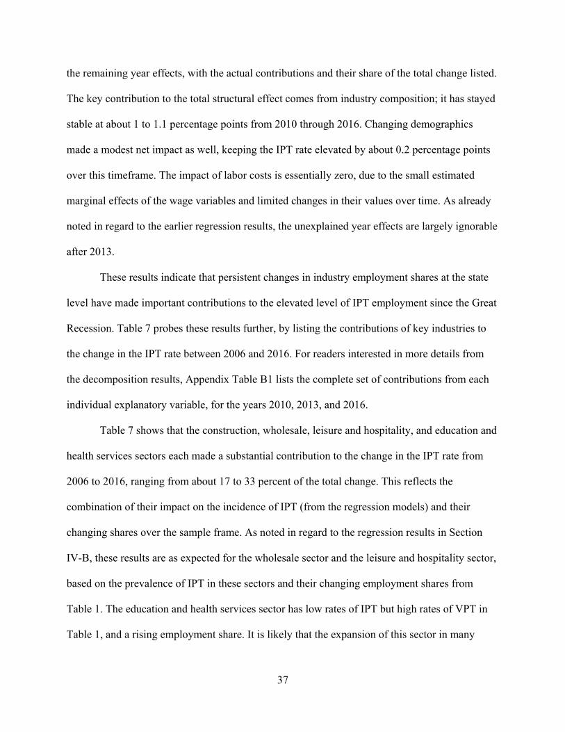
37

the remaining year effects, with the actual contributions and their share of the total change listed.

The key contribution to the total structural effect comes from industry composition; it has stayed

stable at about 1 to 1.1 percentage points from 2010 through 2016. Changing demographics

made a modest net impact as well, keeping the IPT rate elevated by about 0.2 percentage points

over this timeframe. The impact of labor costs is essentially zero, due to the small estimated

marginal effects of the wage variables and limited changes in their values over time. As already

noted in regard to the earlier regression results, the unexplained year effects are largely ignorable

after 2013.

These results indicate that persistent changes in industry employment shares at the state

level have made important contributions to the elevated level of IPT employment since the Great

Recession. Table 7 probes these results further, by listing the contributions of key industries to

the change in the IPT rate between 2006 and 2016. For readers interested in more details from

the decomposition results, Appendix Table B1 lists the complete set of contributions from each

individual explanatory variable, for the years 2010, 2013, and 2016.

Table 7 shows that the construction, wholesale, leisure and hospitality, and education and

health services sectors each made a substantial contribution to the change in the IPT rate from

2006 to 2016, ranging from about 17 to 33 percent of the total change. This reflects the

combination of their impact on the incidence of IPT (from the regression models) and their

changing shares over the sample frame. As noted in regard to the regression results in Section

IV-B, these results are as expected for the wholesale sector and the leisure and hospitality sector,

based on the prevalence of IPT in these sectors and their changing employment shares from

Table 1. The education and health services sector has low rates of IPT but high rates of VPT in

Table 1, and a rising employment share. It is likely that the expansion of this sector in many

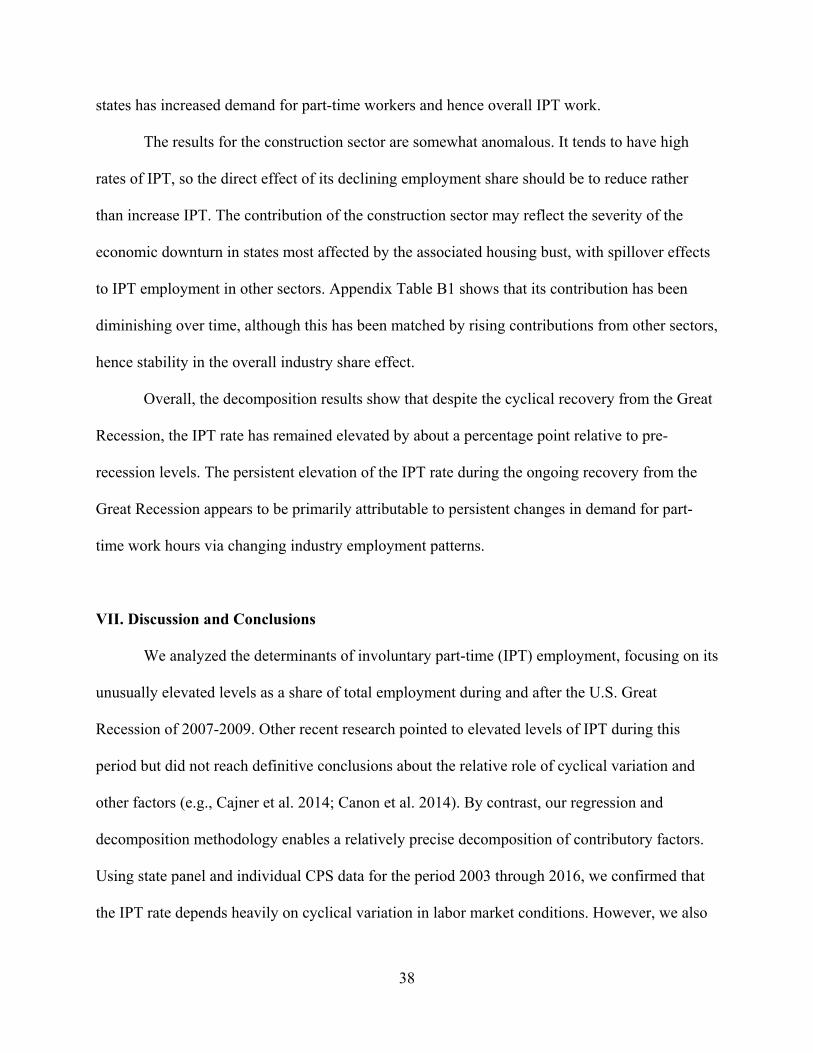
38

states has increased demand for part-time workers and hence overall IPT work.

The results for the construction sector are somewhat anomalous. It tends to have high

rates of IPT, so the direct effect of its declining employment share should be to reduce rather

than increase IPT. The contribution of the construction sector may reflect the severity of the

economic downturn in states most affected by the associated housing bust, with spillover effects

to IPT employment in other sectors. Appendix Table B1 shows that its contribution has been

diminishing over time, although this has been matched by rising contributions from other sectors,

hence stability in the overall industry share effect.

Overall, the decomposition results show that despite the cyclical recovery from the Great

Recession, the IPT rate has remained elevated by about a percentage point relative to pre-

recession levels. The persistent elevation of the IPT rate during the ongoing recovery from the

Great Recession appears to be primarily attributable to persistent changes in demand for part-

time work hours via changing industry employment patterns.

VII. Discussion and Conclusions

We analyzed the determinants of involuntary part-time (IPT) employment, focusing on its

unusually elevated levels as a share of total employment during and after the U.S. Great

Recession of 2007-2009. Other recent research pointed to elevated levels of IPT during this

period but did not reach definitive conclusions about the relative role of cyclical variation and

other factors (e.g., Cajner et al. 2014; Canon et al. 2014). By contrast, our regression and

decomposition methodology enables a relatively precise decomposition of contributory factors.

Using state panel and individual CPS data for the period 2003 through 2016, we confirmed that

the IPT rate depends heavily on cyclical variation in labor market conditions. However, we also

39

identify slower moving market factors, reflected mainly in industry employment shares, which

account for ongoing elevation in the IPT rate despite the cyclical recovery in the labor market.

These market or structural factors account for about a percentage point or more of the elevated

IPT share of total employment through 2016, with very little change in their overall contribution

since the recovery began in 2010. These results suggest that the incidence of IPT employment is

likely to remain somewhat elevated in the future as well.

As we noted earlier, similar patterns in IPT and part-time work more generally have been

observed for other countries, suggesting that the determinants reflect broad labor market

developments rather than institutional specifics. For example, the analysis of Borowczyk-Martins

and Lalé (2017) uncovered shared patterns in labor market flows that contributed to recent

elevation in IPT work in the United States and the United Kingdom. Additional international

comparisons could prove quite informative with respect to the structural determinants of IPT. In

particular, assessing the role of shared market factors will help shed light on the possible role of

institutional specifics such as the ACA employer mandate in the United States, on which the

direct evidence currently is mixed. We also uncovered suggestive evidence of links between

rising IPT and work in the informal gig economy, despite the poor measurement of the latter in

CPS data (Abraham et al. 2017). Further investigation using data sources that provide more

precise and accurate information on informal gig work, such as linked tax data or original

surveys, may prove useful to shed further light on such links.

Our framework and findings suggest other avenues for future work as well. We focused

on recent empirical patterns in involuntary part-time work, discussing a market demand and

supply framework in broad conceptual terms to guide our empirical analyses. More formal

modeling of the demand and supply sides of the market for part-time work, and its general

40

equilibrium properties, could be quite valuable for refining these findings. The wage effects of

such changes are of particular interest and perhaps could be identified by focusing on industries

with high incidence of part-time work, such as the retail and hospitality sectors. Accounting for

the frictions that divide part-time workers into involuntary and voluntary groups is an especially

interesting challenge for estimation of changes in the part-time wage penalty and may have

important implication for movements in aggregate wages as well (as in Daly and Hobijn 2016).

41

References

Abhayaratna, Joanna, Les Andrews, Hudan Nuch, and Troy Podbury. 2008. "Part Time Employment: The Australian Experience." Australian Government Productivity Commission Staff Working Paper.

Abraham, Katharine G., John C. Haltiwanger, Kristin Sandusky, and James R. Spletzer. 2017. “Measuring the Gig Economy: Current Knowledge and Open Issues.” Working paper, University of Maryland, March.

Baker, Scott R., Nicholas Bloom, and Steven J. Davis. 2016. “Measuring Economic Policy Uncertainty.” Quarterly Journal of Economics 131 (4, Nov.): 1593-1636.

Bell, David N.F., and David G. Blanchflower. 2014. “Commentary: Labour Market Slack in the UK.” National Institute Economic Review No. 229, August.

Bitler, Marianne, and Hilary Hoynes. 2016. “The More Things Change, the More They Stay the Same? The Safety Net and Poverty in the Great Recession.” Journal of Labor Economics 34(1, part 2): S403-444.

Blanchflower, David G., and Andrew T. Levin. 2015. “Labor Market Slack and Monetary Policy.” NBER Working Paper 21094, April.

Borowczyk-Martins, Daniel, and Etienne Lalé. 2016. “The Rise of Part-time Employment.” Working paper, Copenhagen Business School and University of Bristol, July.

Borowczyk-Martins, Daniel, and Etienne Lalé. 2017. “Employment Adjustment and Part-time Work: Lessons from the United States and the United Kingdom.” Working paper, Copenhagen Busines School and Université du Québec à Montréal, December.

Borowczyk-Martins, Daniel, and Etienne Lalé. 2018. “The Welfare Effects of Involuntary Part-time Work.” Oxford Economic Papers 70(1, Jan.): 183–205

Bracha, Anat, and Mary A. Burke. 2017. “Who Counts as Employed? Informal Work, Employment Status, and Labor Market Slack.” Working Paper 17-18, Opportunity & Inclusive Growth Institute, Federal Reserve Bank of Minneapolis. June.

Buchmueller, Thomas C, John DiNardo, and Robert G Valletta. 2011. "The Effect of an Employer Health Insurance Mandate on Health Insurance Coverage and the Demand for Labor: Evidence from Hawaii." American Economic Journal-Economic Policy 3(4): 25-51.

Cajner, Tomaz, Dennis Mawhirter, Christopher Nekarda, and David Ratner. 2014. "Why Is Involuntary Part-Time Work Elevated?" In FEDS Notes: Board of Governors of the Federal Reserve System.

42

Canon, Maria E, Marianna Kudlyak, Guannan Luo, and Marisa Reed. 2014. "Flows to and from Working Part Time for Economic Reasons and the Labor Market Aggregates During and after the 2007-09 Recession." Federal Reserve Bank of Richmond Economic Quarterly 100(2): 87-111.

Carrington, William J, Kristin McCue, and Brooks Pierce. 2002. "Nondiscrimination Rules and the Distribution of Fringe Benefits." Journal of Labor Economics 20(2): S5-S33.

Cassidy, Natasha, and Stephanie Parson. 2017. “The Rising Share of Part-time Employment.” Reserve Bank of Australia Bulletin, September Quarter: 19-26.

Chang, Yongsung, Sun-Bin Kim, Kyooho Kwon, and Richard Rogerson. 2011. "Interpreting Labor Supply Regressions in a Model of Full- and Part-Time Work." American Economic Review 101(3): 476-81.

Daly, Mary C., and Bart Hobijn. 2014. “Downward Nominal Wage Rigidities Bend the Phillips Curve.” Journal of Money, Credit, and Banking 46(S2): 51-93.

Daly, Mary C., and Bart Hobijn. 2016. “The Intensive and Extensive Margins of Real Wage Adjustment.” FRBSF Working Paper 2016-04, March.

Daly, Mary C., and Robert G. Valletta. 2006. “Inequality and Poverty in the United States: The Effects of Rising Dispersion of Men’s Earnings and Changing Family Behavior.” Economica 73(Feb.): 75-98

Dillender, Marcus, Carolyn J. Heinrich, and Susan N. Houseman. 2016. “Effects of the Affordable Care Act on Part-Time Employment: Early Evidence. Upjohn Institute Working Paper 16-258. Kalamazoo, MI.

DiNardo, John, Nicole M. Fortin, and Thomas Lemieux. 1996. “Labor Market Institutions and the Distribution of Wages, 1973-1992: A Semiparametric Approach.” Econometrica 64 (5): 1001–1044.

Dolfin, Sarah. 2006. "An Examination of Firms' Employment Costs." Applied Economics 38(8): 861-78.

Euwals, Rob, and Maurice Hogerbrugge. 2006. "Explaining the Growth of Part‐Time Employment: Factors of Supply and Demand." Labour 20(3): 533-57.

Even, William E., and David A. Macpherson. 2017. “The Affordable Care Act and the Growth of Involuntary Part-Time Employment.” Working paper, Trinity University, August.

Fallick, Bruce. 1999. “Part-time work and industry growth.” Monthly Labor Review, March 1999: 22-29.

Friesen, Jane. 1997. “The Dynamic Demand for Part-Time and Full-Time Labour.” Economica 64 (Aug.): 495-507.

43

Garrett, Bowen A., Robert Kaestner, and Anuj Gangopadhyaya. 2017. “Recent Evidence on the ACA and Employment: Has the ACA Been a Job Killer? 2016 Update.” Report, The Urban Institute, February.

Golden, Lonnie. 2016. “Still falling short on hours and pay.” Report, Economic Policy Institute, Washington, DC. December 5.

Hirsch, Barry T. 2005. "Why Do Part-Time Workers Earn Less? The Role of Worker and Job Skills." Industrial & Labor Relations Review 58(4): 525-51.

International Monetary Fund. 2017. “Seeking Sustainable Growth: Short-Term Recovery, Long-Term Challenges.” World Economic Outlook, October. Washington, DC.

Katz, Lawrence F., and Alan B. Krueger. 2016. "The Rise and Nature of Alternative Work Arrangements in the United States, 1995-2015." NBER Working Paper 22667, September; revised June 2017.

Leppel, Karen, and Suzanne Heller Clain. 1988. “The growth in involuntary part-time employment of men and women.” Applied Economics 20: 1155-66.

Leppel, Karen, and Suzanne Heller Clain. 1993. “Determinants of Voluntary and Involuntary Part-Time Employment.” Eastern Economic Journal 19(1, Winter): 59-70.

Lettau, Michael K, and Thomas C. Buchmueller. 1999. "Comparing Benefit Costs for Full- and Part-Time Workers." Monthly Labor Review 122(3): 30-35.

Mathur, Aparna, Sita Nataraj Slavova, and Michael R. Strain. 2016. “Has the Affordable Care Act increased part-time employment?” Applied Economics Letters 23(3): 222-225.

Moriya, Asako S., Thomas M. Selden, and Kosali I. Simon. 2016. “Little Change Seen In Part-Time Employment as a Result of the Affordable Care Act.” Health Affairs 35(1): 119–123.

Papke, Leslie E., and Jeffrey M. Wooldridge. 2008. “Panel data methods for fractional response variables with an application to test pass rates.” Journal of Econometrics (145): 121-133.

Polivka, Anne, and Stephen Miller. 1998. “The CPS After the Redesign: Refocusing the Economic Lens.” In Labor Statistics Measurement Issues, eds. John Haltiwanger, Marilyn Manser, and Robert Topel. Chicago: University of Chicago Press, pp. 249–289.

Robertson, John, and Ellyn Terry. 2014. “Part-Time for Economic Reasons: A Cross-Industry Comparison” FRB Atlanta Macroblog, July 18.

Stratton, Leslie S. 1996. “Are `Involuntary’ Part-Time Workers Indeed Involuntary?” Industrial and Labor Relations Review 49(3, April): 522-36.

Tilly, Chris. 1991. "Reasons for the Continuing Growth of Part-Time Employment." Monthly Labor Review 114(3): 10-18.

44

Valletta, Robert G, and Leila Bengali. 2013. "What’s Behind the Increase in Part-Time Work?" FRBSF Economic Letter 2013-24, August 26.

Valletta, Robert G, and Catherine van der List. 2015. "Involuntary Part-Time Work: Here to Stay?" FRBSF Economic Letter 2015-19, June 8.

Yellen, Janet. 2014. “Labor Market Dynamics and Monetary Policy.” Speech at the FRB Kansas City Economic Symposium, Jackson Hole, Wyoming, August 22.

45

Figure 1

0

5

10

15

20

25

1994 1998 2002 2006 2010 2014

Source: BLS (seasonally adjusted data). Part-time rates expressed as a share of total civilian employment. Gray areas are recessions.

Part-time Work by Type (share of total employment), Jan. 1994-Dec. 2016

Involuntary Part-Time

Voluntary Part-Time

Part-Time (total)

Percent

Dec. 2016

46

Figure 2 Panel A

Panel B

0

2

4

6

8

10

12

1994 1998 2002 2006 2010 2014

Source: BLS (seasonally adjusted data). Involuntary part-time rate expressed as a share of total civilian employment. Gray areas are recessions.

Involuntary Part-Time Rate vs. Unemployment Rate, Jan. 1994-Dec. 2016 Percent

Unemployment Rate

Involuntary Part-Time Rate

Dec. 2016

0

2

4

6

8

10

12

1994 1998 2002 2006 2010 2014Source: BLS (seasonally adjusted data). IPT component rates expressed as a share of total civilian employment. Gray areas are recessions.

Unemployment and Involuntary Part-Time (IPT) Components, Jan. 1994-Dec. 2016 Percent

Unemployment Rate

IPT: Slack Work

IPT: Could only find PT Work

Dec. 2016

47

Figure 3

AL

HI NV

CA

02

46

81

0IP

T E

mpl

oym

ent

Rat

e (%

)

0 5 10 15Unemployment Rate (%)

Panel A: 2005

AL

HINV

CA

02

46

81

0IP

T E

mpl

oym

ent

Rat

e (%

)

0 5 10 15Unemployment Rate (%)

Panel B: 2010

ALHI

NVCA

02

46

81

0IP

T E

mpl

oym

ent

Rat

e (%

)

0 5 10 15Unemployment Rate (%)

Panel C: 2016

02

46

81

0IP

T E

mpl

oym

ent

Rat

e (%

)

0 5 10 15Unemployment Rate (%)

Panel D: All years (2003-16)

Source: BLS and authors' calculations. IPT employment rate measured as a share of civilian employment. Fitted lines weighted by state employment.

Involuntary Part-Time (IPT) Work and Unemployment, All States (by periods)

48

Figure 4

0.1

.2.3

.4fr

actio

n of

sta

tes

0 2 4 6 8 10IPT Rate (%)

Panel A: Average, 2006 through 2016

0.1

.2.3

.4fr

actio

n of

sta

tes

0 2 4 6 8 10IPT Rate (% point change)

Panel B: Change, 2010 minus 2006

0.1

.2.3

.4fr

actio

n of

sta

tes

-8 -6 -4 -2 0 2IPT Rate (% point change)

Panel C: Change, 2016 minus 2010

0.1

.2.3

.4fr

actio

n of

sta

tes

-4 -2 0 2 4 6IPT Rate (% point change)

Panel D: Change, 2016 minus 2006

Source: BLS and authors' calculations. IPT employment rate measured as a share of civilian employment.

Sub-period levels and changes

Distribution of IPT Employment Rates across States

49

Figure 5

0.0

5.1

.15

.2.2

5fr

actio

n of

sta

tes

0 2 4 6 8 10 12Unemployment Rate (%)

Panel A: Average, 2006 through 2016

0.0

5.1

.15

.2.2

5fr

actio

n of

sta

tes

0 2 4 6 8 10 12Unemployment Rate (% point change)

Panel B: Change, 2010 minus 2006

0.0

5.1

.15

.2.2

5fr

actio

n of

sta

tes

-10 -8 -6 -4 -2 0 2Unemployment Rate (% point change)

Panel C: Change, 2016 minus 2010

0.0

5.1

.15

.2.2

5fr

actio

n of

sta

tes

-6 -4 -2 0 2 4 6Unemployment Rate (% point change)

Panel D: Change, 2016 minus 2006

Source: BLS and authors' calculations.

Sub-period levels and changes

Distribution of Unemployment Rates across States

50

Figure 6

.02

.03

.04

.05

.06

.07

em

plo

ymen

t sh

are

2004 2006 2008 2010 2012 2014 2016year

IPT Rate

Cyclical variation

Structural variation

Note: Authors' calculations based on decomposition applied to regression results from column 1 of Table 3; components measuredrelative to 2006 (see text for details). Year effects excluded. Series are measured as shares of civilian employment. Gray areadenotes recession (approximate).

Actual and estimated components

Involuntary Part-Time Employment (IPT), 2003-16

51

(1) (2) (3) (4) (5) (6) (7) (8) (9) (10) (11) (12)

2005 2010 2016 2005 2010 2016 2005 2010 2016 2005 2010 2016Individual CharacteristicsAll Workers 0.032 0.066 0.041 0.143 0.136 0.142 0.175 0.203 0.182 1.000 1.000 1.000

All 16-24 0.058 0.117 0.075 0.353 0.357 0.367 0.411 0.474 0.442 0.143 0.125 0.127Men 25-34 0.032 0.072 0.040 0.039 0.043 0.048 0.071 0.115 0.089 0.123 0.121 0.123

Women 25-34 0.036 0.069 0.044 0.156 0.139 0.140 0.192 0.208 0.184 0.100 0.103 0.106Men 35-54 0.023 0.053 0.029 0.025 0.025 0.029 0.048 0.078 0.058 0.251 0.240 0.225

Women 35-54 0.029 0.061 0.039 0.156 0.144 0.143 0.185 0.205 0.181 0.227 0.220 0.201All 55-64 0.025 0.053 0.034 0.138 0.126 0.122 0.163 0.179 0.156 0.125 0.151 0.165

All 65+ 0.023 0.043 0.027 0.444 0.386 0.360 0.467 0.429 0.387 0.031 0.040 0.053

Single man 0.047 0.092 0.057 0.138 0.130 0.139 0.185 0.222 0.196 0.216 0.217 0.233Single woman 0.044 0.085 0.056 0.211 0.197 0.210 0.255 0.282 0.266 0.225 0.231 0.241

Married man 0.019 0.046 0.023 0.045 0.047 0.050 0.063 0.093 0.073 0.312 0.303 0.292Married woman 0.025 0.051 0.030 0.212 0.195 0.189 0.237 0.246 0.219 0.246 0.249 0.234

Education LevelLess than High School 0.065 0.138 0.076 0.239 0.212 0.250 0.305 0.350 0.326 0.115 0.093 0.083

High School 0.038 0.085 0.057 0.120 0.117 0.128 0.159 0.202 0.185 0.300 0.283 0.262Some College 0.028 0.063 0.040 0.170 0.171 0.176 0.198 0.234 0.216 0.291 0.295 0.292

Bachelor's 0.018 0.036 0.024 0.106 0.101 0.100 0.124 0.137 0.124 0.195 0.216 0.231More than Bachelor's 0.014 0.025 0.016 0.097 0.098 0.098 0.111 0.123 0.114 0.098 0.113 0.132

Race/ethnicityWhite 0.027 0.055 0.033 0.159 0.150 0.152 0.186 0.205 0.185 0.698 0.683 0.637Black 0.045 0.077 0.056 0.101 0.104 0.118 0.146 0.181 0.173 0.110 0.111 0.120

Hispanic 0.050 0.116 0.061 0.103 0.101 0.124 0.153 0.217 0.185 0.125 0.137 0.152Asian/Pacific Islander 0.026 0.055 0.031 0.119 0.111 0.118 0.145 0.166 0.149 0.046 0.050 0.063

Other 0.046 0.092 0.057 0.148 0.141 0.162 0.193 0.233 0.220 0.021 0.020 0.028Self employment and multiple jobs

Self-employed (unincorporated) 0.056 0.131 0.079 0.211 0.211 0.239 0.267 0.342 0.318 0.068 0.064 0.058Multiple job holders 0.024 0.046 0.033 0.107 0.099 0.109 0.131 0.146 0.142 0.053 0.050 0.050

Self-employed on second job3 0.023 0.045 0.029 0.076 0.082 0.096 0.099 0.127 0.126 0.224 0.199 0.183

(continued)

Demographics: age by gender

Demographics: marital status by gender (all ages)

Table 1: Part-Time Work by Labor Market Group and Sector

(incidence by group)1

Involuntary Part-time Workers Voluntary Part-Time WorkersSum: Involuntary + Voluntary

Part-Time WorkersMemo:

Employment Share2

52

(1) (2) (3) (4) (5) (6) (7) (8) (9) (10) (11) (12)

2005 2010 2016 2005 2010 2016 2005 2010 2016 2005 2010 2016Individual CharacteristicsAll Workers 0.032 0.066 0.041 0.143 0.136 0.142 0.175 0.203 0.182 1.000 1.000 1.000Broad Industry

Mining 0.006 0.013 0.018 0.016 0.012 0.020 0.022 0.025 0.038 0.004 0.005 0.005Construction 0.057 0.135 0.059 0.054 0.048 0.055 0.110 0.183 0.113 0.077 0.062 0.066

Manufacturing 0.017 0.035 0.017 0.035 0.036 0.039 0.053 0.071 0.056 0.121 0.107 0.107Wholesale Trade 0.016 0.032 0.017 0.057 0.053 0.061 0.074 0.085 0.078 0.033 0.028 0.024

Retail Trade 0.042 0.101 0.069 0.231 0.216 0.225 0.273 0.317 0.294 0.120 0.117 0.112Transportation/comm/utilities 0.026 0.052 0.035 0.068 0.065 0.076 0.094 0.116 0.111 0.053 0.052 0.054

Information 0.021 0.040 0.025 0.111 0.105 0.093 0.132 0.145 0.118 0.025 0.023 0.019Financial activities 0.012 0.027 0.014 0.101 0.083 0.086 0.113 0.110 0.100 0.073 0.068 0.070

Professional/business services 0.039 0.067 0.038 0.125 0.109 0.106 0.163 0.176 0.144 0.099 0.108 0.119Leisure & hospitality 0.065 0.137 0.088 0.304 0.283 0.301 0.369 0.420 0.389 0.086 0.091 0.094

Education & health services 0.025 0.046 0.032 0.187 0.173 0.176 0.212 0.219 0.208 0.210 0.236 0.232Other services4 0.045 0.088 0.053 0.230 0.213 0.228 0.274 0.301 0.282 0.050 0.049 0.048

Public administration 0.007 0.018 0.010 0.045 0.047 0.050 0.052 0.064 0.060 0.049 0.054 0.048Broad Occupation

Management, business, financial 0.009 0.021 0.011 0.059 0.054 0.058 0.068 0.075 0.070 0.133 0.140 0.155Professional and related 0.019 0.034 0.022 0.141 0.133 0.128 0.160 0.167 0.150 0.205 0.224 0.232

Services5 0.060 0.117 0.079 0.258 0.237 0.257 0.318 0.353 0.336 0.168 0.182 0.181

Sales and related 0.037 0.085 0.056 0.213 0.203 0.213 0.250 0.287 0.270 0.114 0.109 0.104Office and administrative support 0.023 0.054 0.034 0.166 0.149 0.159 0.189 0.203 0.193 0.144 0.136 0.122

Farming, fishing, forestry 0.069 0.092 0.029 0.096 0.063 0.082 0.165 0.155 0.111 0.001 0.001 0.001Construction and extraction 0.064 0.147 0.065 0.041 0.037 0.041 0.105 0.184 0.106 0.065 0.051 0.052

Installation, maintenance, repair 0.020 0.049 0.024 0.040 0.039 0.042 0.059 0.088 0.066 0.038 0.036 0.033Production 0.028 0.058 0.030 0.050 0.053 0.057 0.078 0.111 0.087 0.070 0.061 0.059

Transportation and material moving 0.041 0.084 0.056 0.116 0.114 0.131 0.157 0.198 0.187 0.062 0.060 0.062

5 Includes healthcare support, protective, food preparation and serving, maintenance, and personal services.

Involuntary Part-time Workers Voluntary Part-Time WorkersSum: Involuntary + Voluntary

Part-Time WorkersMemo:

Employment Share2

2 Share of row group in total employment (part-time and full-time).3 Calculated for multiple job holders; data available for CPS outgoing rotation groups (quarter sample) only. Employment share measured as a fraction of multiple job holders.4 Includes repair/maintenance, personal services, and membership organizations.

Table 1 (continued): Part-Time Work (incidence by group)

Note: Authors' calculations using CPS microdata (with survey sampling weights). Sample includes nonagricultural wage and salary or self-employed (unincorporated) workers age 16 and over who worked positive hours in the survey week and whose hours data were not allocated.

1 Numbers in the first six columns represent the share of all employed individuals for the row category who are in the column category of part-time work (by year).

53

 

Variables(by category) (1) (2) (3) (4) (5)Cyclical

Unemployment Rate (fraction) 0.413*** 1.020*** - 1.026*** 0.994***

(0.032) (0.115) (0.109) (0.109)(Unemp Rate Squared)*10 - -0.338*** - -0.337*** -0.332***

(0.066) (0.067) (0.065)Employment/population ratio (fraction) - - -0.207*** 0.013 0.011

(0.048) (0.030) (0.030)Percentage Change GDP - - - - -0.024***

(0.009)

Year (2006 omitted)

2003 0.002** -0.002* 0.006*** -0.002* -0.001

(0.001) (0.001) (0.001) (0.001) (0.001)2004 0.002*** -0.000 0.004*** -0.000 0.000

(0.001) (0.001) (0.001) (0.001) (0.001)2005 0.001 -0.000 0.002*** -0.000 0.000

(0.001) (0.001) (0.001) (0.001) (0.001)2007 0.002** 0.002*** 0.002* 0.002*** 0.002**

(0.001) (0.001) (0.001) (0.001) (0.001)2008 0.010*** 0.007*** 0.013*** 0.007*** 0.006***

(0.001) (0.001) (0.002) (0.001) (0.001)2009 0.016*** 0.010*** 0.028*** 0.011*** 0.010***

(0.002) (0.002) (0.002) (0.002) (0.002)2010 0.014*** 0.009*** 0.026*** 0.009*** 0.010***

(0.002) (0.002) (0.002) (0.002) (0.002)2011 0.015*** 0.010*** 0.024*** 0.010*** 0.011***

(0.002) (0.002) (0.002) (0.002) (0.002)2012 0.016*** 0.010*** 0.021*** 0.011*** 0.011***

(0.002) (0.002) (0.002) (0.002) (0.002)2013 0.017*** 0.012*** 0.019*** 0.012*** 0.013***

(0.002) (0.002) (0.002) (0.002) (0.002)2014 0.017*** 0.014*** 0.015*** 0.014*** 0.014***

(0.001) (0.001) (0.002) (0.002) (0.002)2015 0.015*** 0.013*** 0.010*** 0.013*** 0.013***

(0.001) (0.001) (0.002) (0.002) (0.002)2016 0.013*** 0.012*** 0.007*** 0.012*** 0.012***

(0.001) (0.001) (0.002) (0.002) (0.002)

State Dummies Yes Yes Yes Yes Yes

Pseudo R20.0151 0.0153 0.0147 0.0153 0.0153

N 714 714 714 714 714

Table 2: Involuntary Part-Time (IPT) Regression Results, 2003-2016: Cyclical Effects(dependent variable is IPT as fraction of state civilian employment; average marginal effects reported)

***p<0.01, **p<0.05, *p<0.10Notes: Standard errors in parentheses (clustered by state). Mean of state civilian employment used for regression weights.

54

 

(1) (2) (3) (4) (5)

Variables(by category)

Baseline specification (with

state market factors)

(1) with labor force rather than

pop shares

(1) with occupation rather than

industry

(1) with occupation

added

(1) with 25th percentile wage

rather than median

Cyclical

Unemployment Rate (fraction) 0.632*** 0.650*** 0.913*** 0.611*** 0.638***

(0.101) (0.098) (0.093) (0.096) (0.101)(Unemp Rate Squared)*10 -0.205*** -0.210*** -0.303*** -0.193*** -0.207***

(0.058) (0.056) (0.054) (0.055) (0.058)

Year (2006 omitted)

2003 0.002 0.002 0.000 0.002 0.001

(0.001) (0.001) (0.001) (0.001) (0.001)2004 0.001 0.001 0.001 0.001 0.001

(0.001) (0.001) (0.001) (0.001) (0.001)2005 0.001 0.001 0.001 0.001 0.001

(0.001) (0.001) (0.001) (0.001) (0.001)2007 0.001 0.001 0.001 0.001 0.001

(0.001) (0.001) (0.001) (0.001) (0.001)2008 0.006*** 0.006*** 0.006*** 0.006*** 0.006***

(0.001) (0.001) (0.001) (0.001) (0.001)2009 0.009*** 0.010*** 0.009*** 0.009*** 0.010***

(0.002) (0.002) (0.003) (0.002) (0.002)2010 0.007** 0.007*** 0.006** 0.007** 0.008***

(0.003) (0.002) (0.003) (0.003) (0.003)2011 0.006* 0.006** 0.005 0.006* 0.007**

(0.003) (0.002) (0.004) (0.003) (0.003)2012 0.005 0.005** 0.004 0.005 0.006**

(0.003) (0.002) (0.004) (0.003) (0.003)2013 0.005 0.004* 0.004 0.004 0.006*

(0.004) (0.003) (0.004) (0.004) (0.003)2014 0.003 0.003 0.005 0.003 0.005

(0.004) (0.003) (0.004) (0.004) (0.004)2015 -0.001 -0.001 0.003 -0.001 0.002

(0.005) (0.003) (0.005) (0.005) (0.005)2016 -0.004 -0.005 0.001 -0.005 -0.002

(0.005) (0.004) (0.005) (0.005) (0.005)

State Market Factors

Labor Costs

ln(median real hourly wage) 0.015 0.012 0.005 0.011 -

(0.014) (0.011) (0.014) (0.014)ln(25th percentile real hourly wage) - - - - 0.001

(0.016)

State Minimum Wage (relative)3-0.003 -0.004 0.004 -0.003 -0.006

(0.011) (0.011) (0.009) (0.011) (0.011)

(continued)

Table 3: Involuntary Part-Time (IPT) Regression Results, 2003-2016: with State Factors(dependent variable is IPT as fraction of state civilian employment; average marginal effects reported)

55

 

   

Table 3 (continued)

(1) (2) (3) (4) (5)

Variables(by category)

Baseline specification (with

state market factors)

(1) with labor force rather than

pop shares

(1) with occupation rather than

industry

(1) with occupation

added

(1) with 25th percentile wage

rather than median

Industry Shares1

Construction -0.276*** -0.206*** - -0.341*** -0.280***

(0.053) (0.061) (0.066) (0.052)Manufacturing 0.029 0.039 - 0.104 0.028

(0.070) (0.073) (0.117) (0.071)Wholesale trade -0.898*** -0.898*** - -0.822*** -0.907***

(0.241) (0.230) (0.264) (0.234)Retail trade -0.130 -0.160 - -0.181 -0.163

(0.131) (0.132) (0.130) (0.131)Transportation/comm/utilities 0.401** 0.419** - 0.372* 0.382**

(0.174) (0.168) (0.202) (0.173)Information -0.155 -0.111 - -0.117 -0.167

(0.187) (0.167) (0.188) (0.185)Financial activities -0.054 0.024 - -0.054 -0.056

(0.132) (0.126) (0.142) (0.130)

-0.096 -0.068 - -0.065 -0.115

(0.080) (0.087) (0.075) (0.080)Leisure & hospitality 0.356*** 0.310*** - 0.404*** 0.341***

(0.122) (0.111) (0.135) (0.117)

0.194** 0.256*** - 0.218*** 0.178**

(0.086) (0.088) (0.082) (0.083)Other services 0.480** 0.485** - 0.542** 0.473**

(0.234) (0.227) (0.212) (0.237)

Population/Labor Force Shares

(age/gender)1,2

All 16-24 -0.008 0.014 0.183* 0.008 -0.003(0.090) (0.041) (0.096) (0.096) (0.089)

Men 25-34 0.415 0.030 0.185 0.455 0.432(0.367) (0.041) (0.416) (0.377) (0.365)

Women 25-34 -0.482 -0.036 -0.143 -0.481 -0.484(0.398) (0.057) (0.480) (0.413) (0.402)

Men 35-54 -0.323 N/A -0.335 -0.303 -0.270(0.308) (0.353) (0.325) (0.326)

Women 35-54 0.024 -0.050 0.008 0.043 -0.006(0.294) (0.064) (0.337) (0.305) (0.295)

All 55-64 0.048 0.002 -0.026 0.050 0.024(0.102) (0.034) (0.113) (0.106) (0.105)

All 65+ -0.109 0.094 0.037 -0.082 -0.129(0.079) (0.060) (0.110) (0.079) (0.079)

(continued)

Professional/business services

Education & health services

56

 

Table 3 (continued)

(1) (2) (3) (4) (5)

Variables(by category)

Baseline specification (with

state market factors)

(1) with labor force rather than

pop shares

(1) with occupation rather than

industry

(1) with occupation

added

(1) with 25th percentile wage

rather than median

Occupation Shares1

Management, business, financial - - 0.020 -0.063 -

(0.089) (0.094)

Professional and related - - 0.018 -0.090 -

(0.090) (0.093)Services - - 0.093 -0.150 -

(0.116) (0.112)Sales and related - - 0.048 -0.097 -

(0.086) (0.087)Office and admin support - - -0.177** -0.106 -

(0.090) (0.107)Farming, fishing, forestry - - -0.452 -0.536* -

(0.333) (0.292)Construction and extraction - - -0.105 -0.031 -

(0.113) (0.102)Installation, maintenance, repair - - 0.021 0.126 -

(0.211) (0.209)Production - - 0.003 -0.228 -

(0.120) (0.153)

State Dummies Yes Yes Yes Yes YesPseudo R2

0.0155 0.0155 0.0154 0.0155 0.0155

N 714 714 714 714 714***p<0.01, **p<0.05, *p<0.101 Omitted categories are as follows: government for the industry categories; transportation and material moving for occupations; individuals age<16 for the population shares; and men age 35-54 for the labor force shares in column 2 (dropping a category is required because the labor force excludes individuals under the age of 16).2 Population shares used in all columns except 2, which uses labor force shares.3 Minimum wage measured relative to state median wage (both nominal).Notes: Standard errors in parentheses (clustered by state). Mean of state civilian employment used for regression weights.

57

(1a) (1b) (2a) (2b) (3a) (3b) (4a) (4b)

Involuntary Part Time

Voluntary Part Time

Involuntary Part Time

Voluntary Part Time

Involuntary Part Time

Voluntary Part Time

Involuntary Part Time

Voluntary Part Time

Cyclical 0.689*** -0.898** 0.672*** 0.075 0.872*** -0.008 0.843*** -0.032

(0.142) (0.358) (0.135) (0.283) (0.085) (0.166) (0.079) (0.093) -0.129* 0.324 -0.163** -0.091 -0.302*** -0.061 -0.299*** -0.024(0.079) (0.227) (0.081) (0.194) (0.055) (0.093) (0.049) (0.049)

Year (only 2007 forward shown; 2006 omitted)

2007 0.001** -0.001 0.002*** -0.001 -0.000 -0.003** -0.000 0.000(0.001) (0.001) (0.001) (0.001) (0.001) (0.001) (0.001) (0.001)

2008 0.007*** 0.002 0.008*** -0.003** 0.004*** -0.007*** 0.004*** -0.002(0.001) (0.002) (0.001) (0.001) (0.001) (0.002) (0.001) (0.002)

2009 0.011*** 0.016*** 0.015*** -0.001 0.009*** -0.007 0.006*** 0.002(0.003) (0.006) (0.003) (0.005) (0.002) (0.005) (0.002) (0.003)

2010 0.010*** 0.013** 0.014*** -0.003 0.007** -0.011* 0.003 -0.001(0.003) (0.006) (0.003) (0.005) (0.003) (0.006) (0.002) (0.004)

2011 0.011*** 0.011* 0.015*** -0.004 0.006* -0.012* 0.002 -0.000(0.003) (0.005) (0.003) (0.004) (0.003) (0.007) (0.002) (0.004)

2012 0.012*** 0.007 0.015*** -0.005 0.005* -0.013* 0.001 -0.001(0.002) (0.005) (0.002) (0.004) (0.003) (0.007) (0.002) (0.005)

2013 0.013*** 0.004 0.016*** -0.006** 0.006* -0.015** 0.002 -0.002(0.002) (0.004) (0.002) (0.003) (0.003) (0.007) (0.003) (0.005)

2014 0.013*** 0.000 0.015*** -0.006*** 0.005 -0.015** 0.001 -0.001(0.001) (0.003) (0.001) (0.002) (0.003) (0.007) (0.003) (0.005)

2015 0.012*** -0.003 0.013*** -0.006*** 0.003 -0.016** -0.002 -0.001(0.001) (0.002) (0.001) (0.002) (0.004) (0.008) (0.004) (0.006)

2016 0.010*** -0.002 0.011*** -0.003** 0.000 -0.014* -0.005 0.002(0.001) (0.002) (0.001) (0.002) (0.004) (0.008) (0.004) (0.006)

(continued)

(add state dummies)

Unemployment Rate (fraction)(Unemployment Rate Squared)*10

Table 4: Multinomial Logit Regressions, IPT and VPT, 2003-2016(full time is the omitted category)

(cyclical & year effects only)

(add individual controls) (add state market factors)

58

Table 4 (continued)(1a) (1b) (2a) (2b) (3a) (3b) (4a) (4b)

Involuntary Part-Time

Voluntary Part-Time

Involuntary Part-Time

Voluntary Part-Time

Involuntary Part-Time

Voluntary Part-Time

Involuntary Part-Time

Voluntary Part-Time

Market Factors (State)Labor Costs

- - - - 0.021** 0.084*** 0.019 -0.010(0.009) (0.023) (0.012) (0.020)

- - - - 0.023* 0.046** -0.007 0.011(0.014) (0.023) (0.009) (0.012)

Industry SharesConstruction - - - - -0.079 0.093 -0.256*** -0.138

(0.068) (0.119) (0.048) (0.086)Manufacturing - - - - 0.044 0.197** -0.011 -0.118

(0.028) (0.078) (0.070) (0.104)Wholesale trade - - - - 0.022 0.052 -0.826*** 0.421

(0.106) (0.223) (0.207) (0.417)Retail trade - - - - 0.271*** 0.093 -0.189 0.109

(0.067) (0.217) (0.127) (0.254)- - - - -0.059 -0.334* 0.303* 0.550***

(0.068) (0.187) (0.157) (0.195)Information - - - - 0.350*** 0.422 -0.006 -0.291

(0.102) (0.269) (0.137) (0.287)Financial activities - - - - -0.103** -0.237* -0.136 -0.060

(0.046) (0.123) (0.111) (0.253)- - - - 0.094*** 0.167** 0.010 -0.266**

(0.032) (0.082) (0.074) (0.123)Leisure & hospitality - - - - 0.030 -0.027 0.240** -0.227

(0.032) (0.097) (0.113) (0.201)- - - - 0.038 0.266*** 0.166** -0.131

(0.032) (0.066) (0.068) (0.139)Other services - - - - 0.068 -0.276 0.409** -0.125

(0.089) (0.259) (0.184) (0.324)

(continued)

Transportation/utilities

Professional/business services

Education & health services

ln(median real hourly wage)State Minimum Wage (relative)

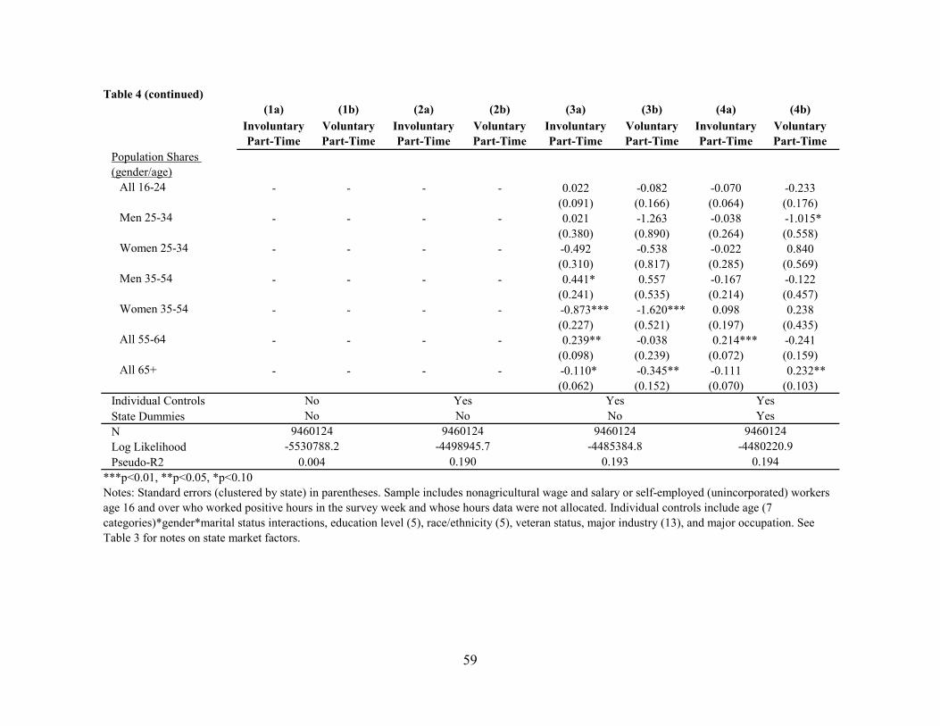
59

Table 4 (continued)(1a) (1b) (2a) (2b) (3a) (3b) (4a) (4b)

Involuntary Part-Time

Voluntary Part-Time

Involuntary Part-Time

Voluntary Part-Time

Involuntary Part-Time

Voluntary Part-Time

Involuntary Part-Time

Voluntary Part-Time

Population Shares (gender/age)

All 16-24 - - - - 0.022 -0.082 -0.070 -0.233(0.091) (0.166) (0.064) (0.176)

Men 25-34 - - - - 0.021 -1.263 -0.038 -1.015*(0.380) (0.890) (0.264) (0.558)

Women 25-34 - - - - -0.492 -0.538 -0.022 0.840(0.310) (0.817) (0.285) (0.569)

Men 35-54 - - - - 0.441* 0.557 -0.167 -0.122(0.241) (0.535) (0.214) (0.457)

Women 35-54 - - - - -0.873*** -1.620*** 0.098 0.238(0.227) (0.521) (0.197) (0.435)

All 55-64 - - - - 0.239** -0.038 0.214*** -0.241(0.098) (0.239) (0.072) (0.159)

All 65+ - - - - -0.110* -0.345** -0.111 0.232**(0.062) (0.152) (0.070) (0.103)

Individual ControlsState DummiesNLog LikelihoodPseudo-R2

YesNo

YesNoYesNo

No Yes

***p<0.01, **p<0.05, *p<0.10Notes: Standard errors (clustered by state) in parentheses. Sample includes nonagricultural wage and salary or self-employed (unincorporated) workers age 16 and over who worked positive hours in the survey week and whose hours data were not allocated. Individual controls include age (7 categories)*gender*marital status interactions, education level (5), race/ethnicity (5), veteran status, major industry (13), and major occupation. See Table 3 for notes on state market factors.

9460124946012494601249460124-5530788.2 -4498945.7 -4485384.8 -4480220.9

0.004 0.190 0.193 0.194

60

(1) (2) (3)

Dependent variable:Self-employed (primary job)

Multiple job holder

Self-employed on

second job1

Explanatory Variables(by category)

State variables

IPT rate 0.163*** 0.168*** 0.045**

(0.046) (0.039) (0.022)Unemployment Rate (fraction) -0.065 0.030 0.029

(0.089) (0.066) (0.040)(Unemp Rate Squared)*10 0.012 -0.045 -0.024

(0.052) (0.039) (0.023)Year (2006 omitted)

2003 0.001 -0.001 -0.000

(0.001) (0.001) (0.000)2004 0.001 -0.000 0.000

(0.001) (0.001) (0.000)2005 0.000 0.000 0.000

(0.001) (0.001) (0.000)2007 -0.002** -0.000 -0.000

(0.001) (0.001) (0.000)2008 -0.005*** -0.002** -0.001**

(0.001) (0.001) (0.000)2009 -0.008*** -0.005*** -0.002***

(0.002) (0.002) (0.001)2010 -0.009*** -0.007*** -0.004***

(0.002) (0.002) (0.001)2011 -0.011*** -0.009*** -0.004***

(0.002) (0.002) (0.001)2012 -0.011*** -0.009*** -0.004***

(0.002) (0.001) (0.001)2013 -0.013*** -0.009*** -0.005***

(0.001) (0.001) (0.001)2014 -0.014*** -0.008*** -0.004***

(0.001) (0.001) (0.001)2015 -0.015*** -0.009*** -0.005***

(0.001) (0.001) (0.001)2016 -0.014*** -0.007*** -0.004***

(0.001) (0.001) (0.000)

Individual Controls2Yes Yes Yes

State Dummies Yes Yes Yes

Pseudo R2 0.0493 0.0241 0.0457N 9460124 9460124 2378758

Table 5: Self-Employment and Multiple Job Holding, Logit Regression Results, 2003-16

(dependent variables as indicated; average marginal effects reported)

***p<0.01, **p<0.05, *p<0.101 Available for multiple job holders, in CPS outgoing rotation groups (quarter sample) only.2 Individual controls same as Table 4 (age/gender/marital, education, race/ethnicity), except industry and occupation categories excluded.Notes: Standard errors in parentheses (clustered by state). Sample includes nonagricultural wage and salary or self-employed (unincorporated) workers age 16 and over who worked positive hours in the survey week and whose hours data were not allocated.

61

(1) (2) (3) (4) (5) (6)

YearTotal change

from 2006

Cyclical component

(unemployment)Industry

compositionAge/gender composition Labor costs Year effects

2006 0.000 0.000 0.000 0.000 0.000 0.000(0.000) (0.000) (0.000) (0.000) (0.000)

2007 0.001 0.000 0.001 0.000 0.000 0.001(0.012) (0.433) (0.178) (0.031) (0.346)

2008 0.012 0.004 0.003 0.001 0.000 0.005(0.325) (0.218) (0.056) (0.004) (0.397)

2009 0.035 0.016 0.009 0.001 0.000 0.009(0.444) (0.248) (0.039) (0.010) (0.258)

2010 0.035 0.017 0.011 0.001 0.000 0.007(0.469) (0.299) (0.034) (0.009) (0.190)

2011 0.033 0.015 0.011 0.002 0.000 0.006(0.446) (0.325) (0.052) (0.006) (0.171)

2012 0.029 0.012 0.011 0.002 0.000 0.004(0.414) (0.370) (0.063) (0.001) (0.152)

2013 0.026 0.010 0.011 0.002 0.000 0.004(0.367) (0.402) (0.074) (0.000) (0.158)

2014 0.020 0.006 0.010 0.002 0.000 0.003(0.270) (0.501) (0.098) -(0.002) (0.133)

2015 0.014 0.002 0.010 0.002 0.000 -0.001(0.166) (0.726) (0.138) (0.011) -(0.040)

2016 0.011 0.001 0.011 0.002 0.000 -0.003(0.087) (1.010) (0.181) (0.028) -(0.305)

Table 6: Decomposition of IPT change (2006 base)

(based on average marginal effects from column 1 of Table 3; fractional contribution to column 1 total in parentheses)

Note: See text (Section VI) for description of decomposition methodology.

62

(1) (2) (3) (4) (5) (6) (7)

Total change from 2006 Construction

Wholesale trade

Transportation/ comm/utilities

Leisure & hospitality

Education & health services

Other services

0.0106 0.0023 0.0018 0.0005 0.0031 0.0035 -0.0001(0.213) (0.165) (0.050) (0.295) (0.328) -(0.005)

Table 7: Decomposition of IPT change (2006 base): Selected Industry Share Effects, 2016 Only

(based on average marginal effects from column 1 of Table 3; fractional contribution to column 1 total in parentheses)

Note: See text (Section VI) for description of decomposition methodology.

63

Appendix A: State Data Sources and Definitions

The definitions and sources for the primary variables used in the state-level panel

analysis (and incorporated into the analyses using CPS individual data) are as follows.

1) Involuntary part-time employment (IPT) rate. We formed this variable using annual

averages from the state labor force and labor underutilization series, available from 2003

forward from the BLS Local Area Unemployment Statistics (LAUS) program:

http://www.bls.gov/lau/stalt_archived.htm. The IPT rate as a share of civilian

employment is calculated by backing it out from the underutilization series U5 and U6

(which includes the IPT group) along with the employment and labor force series.

2) Unemployment rate and labor force participation. These are also obtained from the

BLS LAUS program.

3) State GDP. From the U.S. Bureau of Economic Analysis (BEA) Regional Economic

Accounts.

4) Labor costs:

a) Real median and percentile wage. Median and percentile (25th and 10th) hourly

wage data for each state are from the BLS Occupational Employment Statistics

program (OES, http://www.bls.gov/oes/tables.htm), using data for all occupations for

each year. The wage series are deflated using the BEA’s GDP PCE deflator.

b) Minimum wage. Minimum wages are compiled from the US Department of Labor

minimum wage historical tables

(http://www.dol.gov/whd/state/stateMinWageHis.htm). When there is no listed

minimum wage for a year for a particular state, the most recent listed minimum wage

for that state is used. If there are no data for a state at all or the legislated state

64

minimum is below the U.S. minimum, the U.S. minimum wage is used. When a range

is listed (in the case that different laws apply to different types of enterprises), then

the upper bound is used.

5) Industry employment shares. Calculated using BLS state nonfarm payroll employment

data, available at: http://www.bls.gov/sae/tables.htm.

6) Occupation employment shares. Calculated using data from the BLS Occupational

Employment Statistics program (OES, http://www.bls.gov/oes/tables.htm)

7) Population shares by age/gender. Calculated using the latest available post-censal

population estimates released by the U.S. Bureau of the Census. For example, the 2000s

data use the 2009 vintage of postcensal estimates, and 2010s data use the 2014 vintage.

Historical data are available at http://www.census.gov/popest/data/historical/index.html,

and current estimates are available at http://www.census.gov/popest/data/index.html.

8) Labor force shares by age/gender. From the BLS LAUS, Expanded State Employment

Status Demographic Data (https://www.bls.gov/lau/ex14tables.htm).

65

Appendix B: Supplemental Displays

66

Figure B1

23

45

67

rate

(%

)

2002 2004 2006 2008 2010 2012 2014 2016year

Actual

Adjusted

Panel A: Involuntary Part Time

1213

1415

1617

rate

(%

)

2002 2004 2006 2008 2010 2012 2014 2016year

Actual

Adjusted

Panel B: Voluntary Part Time

Note: Authors' calculations from CPS data. Adjusted series reflects reweighting to hold individualcharacteristics at 2003 distribution (see text). Series are measured as shares of civilian employment.Gray area denotes recession period (approximate).

Part-Time Employment (actual and adjusted)

67

Figure B2

AL

AK

AZ

AR

CA

CO

CT

DE

DCFL

GAHI

ID

IL

IN

IA

KS

KY

LA

ME

MD

MA

MI

MN

MS

MO

MT

NENV

NHNJ

NMNY

NC

ND

OH

OK

OR

PARI

SC

SD TN

TXUT

VT

VA

WA

WVWI

WY

22.

53

3.5

44.

5IP

T E

mpl

oym

ent R

ate

(%)

3 4 5 6 7Unemployment Rate (%)

2005

AL

AK

AZ

AR

CA

COCT

DE

DC

FL

GA

HI

IDIL

IN

IA

KS

KY

LA

ME

MD

MA

MI

MN

MSMO

MT

NE

NV

NH NJNM

NY

NC

ND

OH

OK

OR

PA

RI

SC

SD

TN

TXUT

VT

VA

WA

WV

WI

WY

24

68

10IP

T E

mpl

oym

ent R

ate

(%)

4 6 8 10 12 14Unemployment Rate (%)

2010

AL

AKAZ

AR

CA

CO

CT

DE

DC

FL

GA

HI ID

IL

IN

IA

KS

KY

LA

ME

MDMA

MI

MN

MS

MO

MT

NE

NV

NH

NJ

NM

NY

NC

ND

OH

OK

OR

PARI

SC

SD

TN

TXUT

VT

VAWA WV

WI

WY

23

45

6IP

T E

mpl

oym

ent

Rat

e (%

)

3 4 5 6 7Unemployment Rate (%)

2016

24

68

10IP

T E

mpl

oym

ent

Rat

e (%

)

0 5 10 15Unemployment Rate (%)

All years (2003-16)

Source: BLS and authors' calculations. IPT employment rate measured as a share of civilian employment. Fitted lines weighted by state employment.

Involuntary Part-Time (IPT) Work and Unemployment, by State

68

Figure B3

AL

HI

NV

CA

02

46

81

0C

han

ge in

IP

T R

ate

(%

poi

nts

)

0 2 4 6 8 10 12Change in Unemployment Rate (% points)

Panel A: 2010 minus 2006

AL

HI

NVCA

-8-6

-4-2

02

Ch

ange

in I

PT

Rat

e (

% p

oin

ts)

-12 -10 -8 -6 -4 -2 0Change in Unemployment Rate (% points)

Panel B: 2016 minus 2010

ALHI

NV

CA

-20

24

68

Ch

ange

in I

PT

Rat

e (

% p

oin

ts)

-6 -4 -2 0 2 4 6Change in Unemployment Rate (% points)

Panel C: 2016 minus 2006

Source: BLS and authors' calculations. IPT employment rate measured as a share of civilianemployment. Fitted lines weighted by state employment in base year.

Changes over Time, All States (by periods)Involuntary Part-Time (IPT) Work and Unemployment

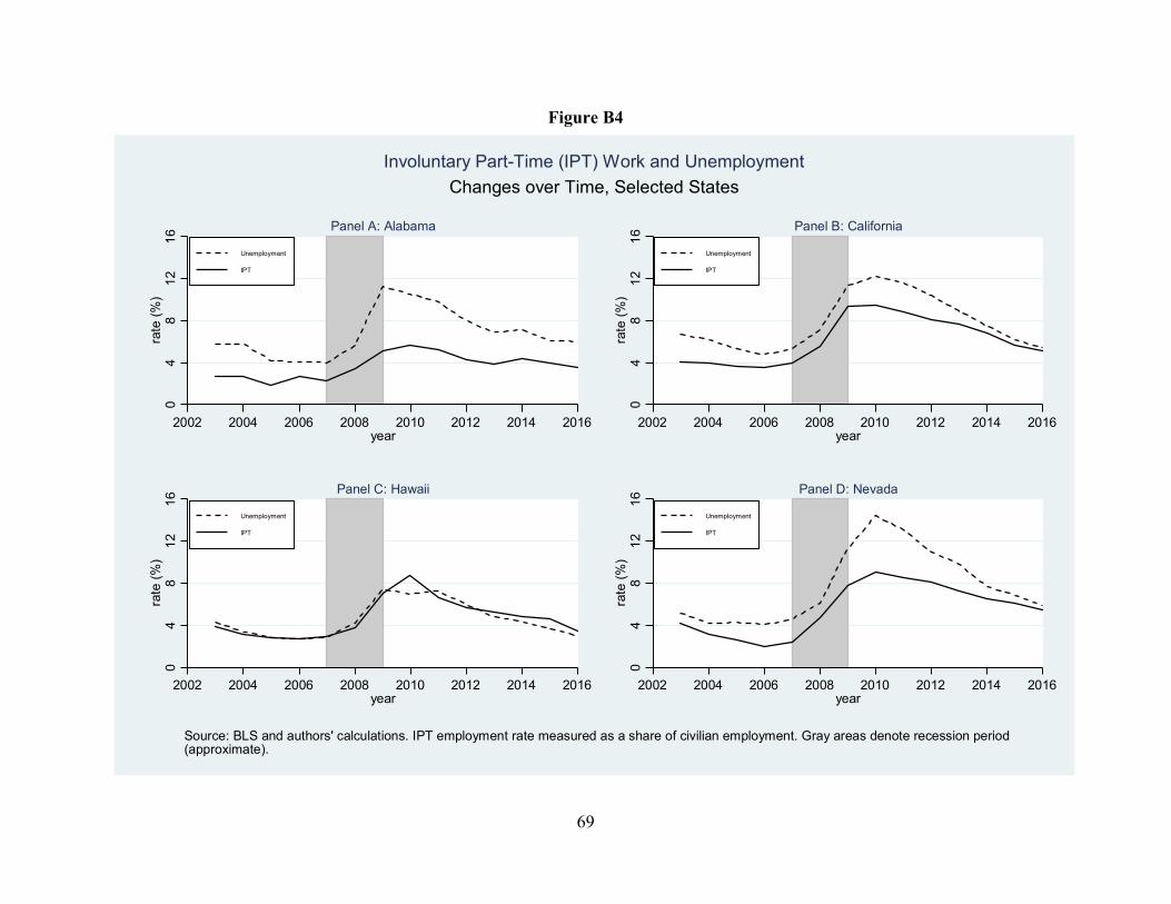
69

Figure B4

04

81

21

6ra

te (

%)

2002 2004 2006 2008 2010 2012 2014 2016year

Unemployment

IPT

Panel A: Alabama

04

81

21

6ra

te (

%)

2002 2004 2006 2008 2010 2012 2014 2016year

Unemployment

IPT

Panel B: California

04

81

21

6ra

te (

%)

2002 2004 2006 2008 2010 2012 2014 2016year

Unemployment

IPT

Panel C: Hawaii

04

81

21

6ra

te (

%)

2002 2004 2006 2008 2010 2012 2014 2016year

Unemployment

IPT

Panel D: Nevada

Source: BLS and authors' calculations. IPT employment rate measured as a share of civilian employment. Gray areas denote recession period(approximate).

Changes over Time, Selected States

Involuntary Part-Time (IPT) Work and Unemployment

70

Figure B5

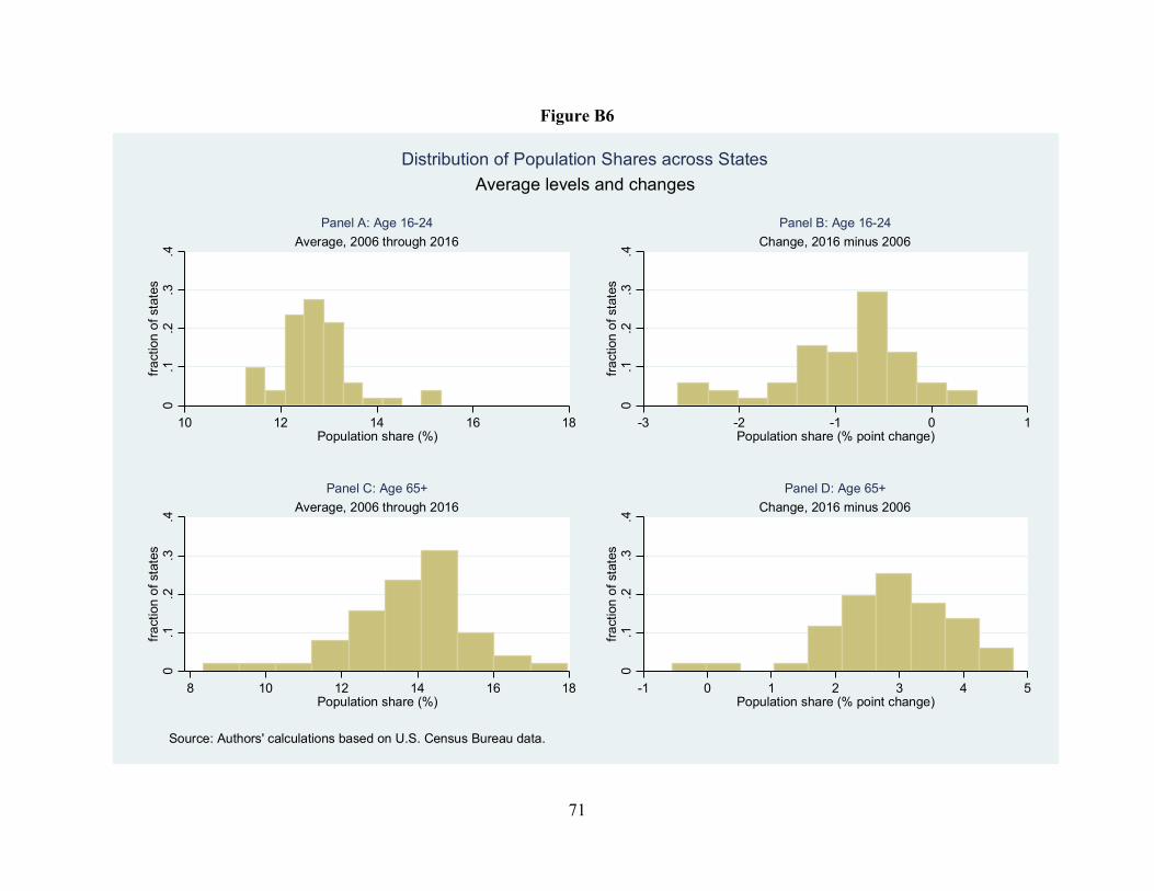
71

Figure B6

0.1

.2.3

.4fr

act

ion

of

stat

es

10 12 14 16 18Population share (%)

Average, 2006 through 2016

Panel A: Age 16-24

0.1

.2.3

.4fr

act

ion

of

stat

es

-3 -2 -1 0 1Population share (% point change)

Change, 2016 minus 2006

Panel B: Age 16-24

0.1

.2.3

.4fr

act

ion

of

stat

es

8 10 12 14 16 18Population share (%)

Average, 2006 through 2016

Panel C: Age 65+

0.1

.2.3

.4fr

act

ion

of

stat

es

-1 0 1 2 3 4 5Population share (% point change)

Change, 2016 minus 2006

Panel D: Age 65+

Source: Authors' calculations based on U.S. Census Bureau data.

Average levels and changes

Distribution of Population Shares across States

72

Figure B7

0.1

.2.3

.4.5

fra

ctio

n o

f st

ates

12 16 20 24 28 32Median wage

Average, 2006 through 2016

Panel A: Median wage

0.1

.2.3

.4.5

fra

ctio

n o

f st

ates

-2 0 2 4 6Median wage (change)

Change, 2016 minus 2006

Panel B: Median wage

0.1

.2.3

.4.5

fra

ctio

n o

f st

ates

.2 .3 .4 .5 .6Minimum wage (relative)

Average, 2006 through 2016

Panel C: Minimum wage (relative)

0.1

.2.3

.4.5

fra

ctio

n o

f st

ates

-.04 0 .04 .08 .12 .16 .2Minimum wage (relative)

Change, 2016 minus 2006

Panel D: Minimum wage (relative)

Source: BLS and authors' calculations. Median wage is inflation adjusted (2016 $), minimum wage measured relative to nominal median wage.

Average levels and changes

Distribution of Median and Minimum Wage across States

73

(1) (2) (3)

Years: 2010 2013 2016

Variables (by category)

Cyclical

Unemployment effects 0.0165 0.0097 0.0009

Industry Shares

Construction 0.0039 0.0032 0.0023

Manufacturing -0.0004 -0.0004 -0.0004

Wholesale trade 0.0012 0.0011 0.0018

Retail trade 0.0002 0.0003 0.0003

Transportation/comm/utilities -0.0002 0.0000 0.0005

Information 0.0002 0.0003 0.0003

Financial activities 0.0001 0.0002 0.0002

Professional/business services -0.0001 -0.0007 -0.0008

Leisure & hospitality 0.0015 0.0027 0.0031

Education & health services 0.0038 0.0038 0.0035

Other services 0.0003 0.0001 -0.0001

Population Shares (age/gender)

All 16-24 0.0000 0.0000 0.0000

Men 25-34 -0.0004 0.0001 0.0006

Women 25-34 -0.0002 -0.0006 -0.0009

Men 35-54 0.0020 0.0035 0.0039

Women 35-54 -0.0001 -0.0003 -0.0003

All 55-64 0.0006 0.0008 0.0008

All 65+ -0.0007 -0.0017 -0.0023

Labor Costs

ln(median real hourly wage) 0.0005 0.0002 0.0004

State Minimum Wage (relative) -0.0002 -0.0002 -0.0001

Year

Year effects 0.0067 0.0042 -0.0032

Appendix Table B1: Full Decomposition of IPT change (2006 base)(based on average marginal effects from column 1 of Table 3)

Note: See text (Section VI) for description of decomposition methodology, plus related results in Tables 6 and 7.