Electronic copy available at: http://ssrn.com/abstract=1731603Electronic copy available at: http://ssrn.com/abstract=1731603Electronic copy available at: http://ssrn.com/abstract=1731603

Charles A. Dice Center for

Research in Financial Economics

Cyclicality, Performance Measurement, and Cash Flow

Liquidity in Private Equity

David T. Robinson,

Duke University, NBER, and SIFR

Berk A. Sensoy,

Department of Finance, The Ohio State University

Dice Center WP 2010-021 Fisher College of Business WP 2011-03-021

Revision date: September 2011

Original date: December 2010

This paper can be downloaded without charge from:

http://www.ssrn.com/abstract=1731603

An index to the working paper in the Fisher College of

Business Working Paper Series is located at: http://www.ssrn.com/link/Fisher-College-of-Business.html

fisher.osu.edu

Fisher College of Business

Working Paper Series

Electronic copy available at: http://ssrn.com/abstract=1731603Electronic copy available at: http://ssrn.com/abstract=1731603Electronic copy available at: http://ssrn.com/abstract=1731603

Cyclicality, Performance Measurement, and Cash FlowLiquidity in Private Equity∗

David T. RobinsonDuke University and NBER

Berk A. SensoyOhio State University

September 8, 2011

Abstract

Public and private equity waves move together. Using quarterly cash flow datafor a large sample of venture capital and buyout funds from 1984-2010, we investigatethe implications of this co-cyclicality for understanding private equity cash flows andperformance. In the cross-section, varying the beta used to assess relative performancehas a large effect near a beta of zero, but only a modest effect for more reasonable betaestimates. For instance, buyout funds outperform the S&P 500 by 18% over the lifeof the fund, and moving to a beta of 1.5 only reduces this to 12%. A similar messagecomes through in the time series. Though funds raised in hot markets underperform inabsolute terms, this underperformance is sharply reduced by a comparison to the S&P500, and disappears entirely at the levels of beta recently estimated in the literature.These findings imply that high private equity fundraising forecasts both low privateequity cash flows and low market returns, suggesting a positive correlation betweenprivate equity net cash flows and public equity valuations. Indeed, while both capitalcalls and distributions rise with public equity valuations, distributions are more sensi-tive than calls, so net cash flows are procyclical and private equity funds are liquidityproviders (sinks) when market valuations are high (low). Venture cash flows and per-formance are considerably more procyclical than buyout. Debt market conditions alsohave a significant impact on cash flows. At the same time, most cash flow variationis idiosyncratic across funds, and most predictable variation is explained by the age ofthe fund.

∗We thank Harry DeAngelo, Tim Jenkinson, Steve Kaplan, Josh Lerner, Andrew Metrick, OguzhanOzbas, Ludovic Phalippou, Antoinette Schoar, Morten Sørensen, Per Stromberg, Rene Stulz, Mike Weis-bach, and seminar and conference participants at Baylor University, Erasmus University Rotterdam, LondonSchool of Economics, Tilburg University, UCSD, the EFA 2011 Annual Meeting, the NBER Entrepreneur-ship Summer Institute, and the third annual LBS Private Equity Symposium for helpful comments anddiscussions. This paper, along with a companion paper, supersedes a previous draft entitled “Private Equityin the 21st Century: Cash flows, Performance and Contract terms from 1984-2010.” Contact information:davidr@duke.edu; sensoy 4@fisher.osu.edu .

Electronic copy available at: http://ssrn.com/abstract=1731603Electronic copy available at: http://ssrn.com/abstract=1731603Electronic copy available at: http://ssrn.com/abstract=1731603

I. Introduction

Private equity has emerged as a major feature of financial markets over the last thirty

years, with tremendous fundraising growth since the mid-1990s. This recent period is also

notable for its episodes of extreme cyclicality, including the venture capital (VC) boom and

bust of the late 1990s and early 2000s, and the buyout boom and bust of the mid- and late

2000s. Private equity cycles broadly mirror those of public equity (and debt) markets. The

most recent VC boom and bust coincided with the broader boom and bust of the internet

era, and the buyout boom of the mid-2000s coincided with high public equity valuations and

a low cost of debt, ending with the financial crisis and recession of 2007-2009.

How does the co-movement of public and private capital markets affect our understanding

of private equity cash flows and returns? In this paper, we focus on two aspects of this ques-

tion. First, we study how co-movement affects inferences about the relative performance of

private equity, both in the cross-section and over time. Second, we investigate how macroe-

conomic fundamentals and overall market conditions impact the behavior of cash flows into

and out of private equity funds, which in turn determine the returns that investors receive.

These questions are important for both practical and theoretical reasons. At the practical

level, investors in a private equity fund are contractually obligated to provide capital to the

fund when it is called (and not, in general, all at once when the investment decision is made),

and in return receive distributions when the fund’s investments are exited. Consequently,

the impact of broader market conditions on the timing and magnitude of these calls and

distributions, which in turn determines whether private equity funds are liquidity providers

or sinks over the business cycle, is essential for understanding the opportunity costs and

benefits of private equity investments relative to other asset classes. In addition to their

practical importance, these questions contribute to a broad research stream in economics

and finance that seeks to understand the covariance of returns across different asset classes,

the implications of this covariance for performance measurement, and the impact of economic

conditions and business cycles on asset cash flows and returns (e.g. Fama and French, 1989).

The chief obstacle hampering study of these questions has been lack of recent data on

private equity cash flows. Our analysis overcomes this obstacle using a proprietary database

1

of quarterly cash flows for 837 buyout and venture capital funds from 1984 to 2010, rep-

resenting almost $600 billion in committed capital. The dataset is the first available for

academic research to include cash flow information for a large sample of private equity funds

raised after the pre-1995 period first studied by Kaplan and Schoar (2005).1

The data come directly from the internal accounting system of a large, anonymous limited

partner, and are free from the self-reporting and survivorship biases that plague standard

private equity databases (Harris, Jenkinson, and Stucke, 2010). The portfolio is also in part

randomly selected, because it was assembled over time through a series of mergers occurring

for reasons unrelated to each company’s private equity exposure. We discuss the coverage

and representativeness of the data in the next section.

We begin with an analysis of the effect of private/public equity return co-movement

on performance inferences. This co-movement is measured by the beta of private equity.

The nature of private equity reporting makes estimating beta a difficult task, even at the

industry level, let alone the fund level. As a result, different studies have reached different

conclusions.2 Given the difficulties and lack of clear consensus, we put forth a complementary

approach that asks how sensitive performance inferences are to beta. We ask the question:

How do inferences about fund performance change if one believes the true beta is 1.5 rather

than 1.0, or that the Nasdaq matches the fund’s systematic risk better than the S&P 500?

To address these questions, we offer two extensions to the public market equivalent (PME)

performance measure pioneered by Kaplan and Schoar (2005). The standard PME compares

a private equity fund’s performance to the S&P 500 by forming the ratio of discounted

distributions to discounted calls, using the S&P return as the discount rate. As Kaplan and

Schoar (2005) point out, this procedure implicitly assumes a beta of one.

Our first extension replaces the S&P benchmark return with narrower indexes more

closely tailored to a fund’s investment strategy. These indexes produce “tailored PMEs”

that allow beta to differ from one implicitly, through the beta of the tailored benchmark.

1The data also include the key terms of the management contract between private equity fund man-agers and their investors, including manager compensation and ownership. We explore issues relating tomanagement contracts in a companion paper, Robinson and Sensoy (2011).

2See Gompers and Lerner (1997), Peng (2001), Woodward and Hall (2003), Cochrane (2005), Kortewegand Sorensen (2010), Jegadeesh, Kraussl, and Pollet (2010), and Driessen, Lin, and Phalippou (2011) forestimates and discussions of the issues.

2

Our second extension explicitly introduces a beta to the PME calculation. By varying

beta, we lever the S&P benchmark return used in the PME calculation, allowing us to trace

out the “levered PME”-beta relation for each fund. The levered PMEs nest as special cases

both the standard PME and the undiscounted ratio of distributions to calls (TVPI).

In the cross-section, we find that moving from a beta of zero (TVPI) to a beta of one

(PME) has a significant impact on performance assessments. The average TVPI for buyout

funds in our sample is 1.57, indicating an unadjusted return of 57% over the life of the fund,

while the average buyout PME is 1.18. However, further increases in beta have strongly

diminishing effects on inferences (i.e., the levered PME-beta relation is convex). In particular,

performance inferences are remarkably insensitive to beta around the levels of beta estimated

from prior work on private equity portfolio companies. Surprisingly, raising the beta to 1.5

(the high end of buyout beta estimates in the literature) lowers the average levered PME

only slightly, to 1.12. Similarly, tailored PMEs offer essentially the same inferences as the

standard PME. Venture capital funds display similar patterns. These results contrast with

intuition from standard asset pricing models used to benchmark the performance of other

asset classes like mutual funds, in which relative performance inferences are linear in beta.

An implication of these analyses is that for many purposes, it may be less important to know

the exact beta than to have a sense of its likely range.

We also apply these tools to performance in the time-series. Kaplan and Stromberg

(2009), investigating buyout funds, find evidence for counter-cyclicality in fundraising and

performance: the absolute performance (IRR) of buyout funds raised in boom fundraising

years is significantly worse than that of funds raised in bust periods. We find the same

pattern, for both buyout and venture, which squares with received wisdom among industry

observers. However, as noted above, private equity fundraising booms and busts are strongly

correlated with public equity booms and busts. This co-cyclicality raises the question of

whether cycles in absolute private equity performance show up intact in cycles in relative

performance, or instead are differenced out by differences in the returns to public equities.

When we replace absolute performance measures with the relative performance measure-

ment implied by PMEs, we find that the underperformance of funds raised in hot markets

vanishes altogether for buyout funds, and is reduced in magnitude by about two-thirds for

3

venture funds. Tracing out the levered PME-fundraising relation, we find that the relation

ceases to be reliably negative above a beta of about 0.5 for buyout funds and about 1.5 for

venture funds. Both of these betas are below recent estimates of portfolio company betas

in the literature (which tend to be in the range of 0.8-1.5 for buyout and 2-3 for venture).

Consequently, at the levels of beta estimated by recent work on portfolio companies, there

is not a negative relationship between private equity fundraising and relative performance.

These results occur because times of high private equity fundraising coincide with public

market booms, and presage broader market downturns.

These findings lead to the second aspect of co-cyclicality that we study, which moves

beyond fund-level performance to the behavior of the cash flows that comprise returns. Our

results on fundraising and performance imply that times of high fundraising activity forecast

both low levels of distributions relative to capital calls and low public market returns (or

discount rates). This in turn suggests that when public market valuations are low, in the

midst of downturns, net cash flows (distributions minus calls) at the fund level are also low.

Examining quarterly calls, distributions, and net cash flows directly, we find that this

is indeed the case. Holding fund age fixed, both capital calls and distributions rise with

public equity valuations.3 We also show that distributions are more sensitive than calls.

Consequently, net cash flows to funds of a given age are procyclical and private equity funds

are liquidity providers (sinks) when public market valuations are high (low).

We also find a significant role for the independent information in debt market conditions

above and beyond public equity conditions. Both calls and distributions are negatively

related to the yield spread, a measure of the cost of financing to private equity firms when

they make investments in portfolio companies and to would-be acquirers of those companies

in subsequent M&A transactions. Distributions are more sensitive than calls, so net cash

flows are negatively related to the yield spread.4 Of course, public equity and debt market

3These results on buyout calls are consistent with theoretical predictions of Axelson, Stromberg, andWeisbach (2009) that buyout investments are procyclical.

4The sensitivity of buyout calls to the yield spread is consistent with and complements Axelson et al.(2010), who show that, conditional on making a buyout investment in a portfolio company, deal leverageand pricing are higher when the yield spread is lower. Our results imply that the likelihood that a buyoutfund makes an investment in the first place is also greater when the yield spread is low. At the same time,the primary channel through which the yield spread affects private equity cash flows is through distributionsrather than calls, as a rising yield spread makes it more difficult to exit investments.

4

conditions reflect, and contain independent information about, underlying macroeconomic

fundamentals (Fama and French, 1989). Our results thus establish, in unprecedented detail

at the level of individual capital calls and distributions, a clear link between private equity

activity and business-cycle variation in broader economic conditions.

At the same time, we find that such business-cycle variables explain only a small fraction

of the predictable variation in private equity cash flows. Further, most variation in cash

flows is not predictable, but is idiosyncratic across funds of a given age at a given point in

time. For example, for buyout funds, fund age and calendar quarter fixed effects explain only

7.9% of the variation in net cash flows, which represents an upper bound on the variation

that is potentially explainable by fund age and macroeconomic variables. This leaves 92.1%

as idiosyncratic variation. Of the 7.9% upper bound, fully 7.2% is explained by fund age

fixed effects alone. Adding market valuation and yield spread variables (instead of time fixed

effects) brings the total to 7.4%. Similar conclusions hold for capital calls and distributions

individually. Thus, by an order of magnitude, lifecycle effects captured by the age of the

fund are a stronger predictor of private equity cash flows than macroeconomic conditions.

All of these cash flow results hold for both venture and buyout, and have important

implications for our understanding of the liquidity properties of private equity as an asset

class. On the one hand, the fact that net cash flows are indeed more negative during broader

market downturns raises the possibility of having to liquidate public equity investments at

unfavorable prices to meet capital calls. In other words, the illiquid nature of private equity

investments, together with their procyclicality, raises the specter of adverse liquidity shocks.

On the other hand, there is little reason to believe that private equity should command a

large liquidity premium. Adverse liquidity events are predictable with a low R2. Moreover,

the large idiosyncratic component of cash flows suggests substantial benefit to diversification

across funds, and most predictable variation is explained by the age of the portfolio. The

broad lesson is that despite the possibility of adverse liquidity shocks, managing the liquidity

exposure implied by a portfolio of private equity funds is largely a matter of diversification

across fund ages and across funds of a given age.

We also find strong differences in cyclicality between buyout and venture funds. Venture

capital calls, distributions, net cash flows, and performance over fundraising cycles all exhibit

5

substantially more cyclicality than in buyout. These findings are consistent with prior work

finding a higher beta of venture portfolio companies compared to buyout, but they are not

implied by this prior work. Higher beta would suggest a greater sensitivity of distributions

to market conditions for a given investment, but might, a priori, be offset in a net cash flow

sense by an even larger sensitivity of capital calls to market conditions. Our results are

consistent with Berk, Green, and Naik (2004), whose theory emphasizes that the real option

properties of venture companies can generate substantial cyclicality.

Our work is most closely related to prior work using earlier data on private equity cash

flows. Kaplan and Schoar (2005) and Phalippou and Gottschalg (2009) use cash flow data

from Venture Economics to provide early estimates of private equity performance. Jones

and Rhodes-Kropf (2003) use the same data to investigate how private equity returns relate

to idiosyncratic risk. Ljungqvist and Richardson (2003) and Ljungqvist, Richardson, and

Wolfenzon (2007) use a different sample of buyout funds for which they have data on cash

flows for the full LP-GP-portfolio company chain. They focus on understanding how portfolio

companies and the timing of investments vary across funds and over a fund’s lifecycle. In all

of these papers, the cash flow data ends by 2003, and is limited to funds with vintage years

prior to 1995.

Our work is also related to work studying aspects of cyclicality in private equity (cf.

Kaplan and Schoar (2005), Gompers et al. (2008), Axelson, Stromberg, and Weisbach (2009),

and Kaplan and Stromberg (2009)). No prior work either investigates cyclicality in fund-level

cash flows or examines the impact of public and private equity co-movement on private equity

performance inferences. In its broadest goals, our paper adds to this literature in taking

early steps toward integrating private equity into the broad research stream in economics

and finance that seeks to understand the impact of business cycles on asset returns and

the predictability of payoffs to risky assets. The fundamental illiquidity of private equity

investments makes private equity a unique and challenging setting for investigating these

central questions in asset pricing.

The remainder of the paper proceeds as follows. Section II describes the data. Section III

develops the tailored and levered PME tools, and presents our results on performance infer-

ence and co-movement in the cross-section. Section IV applies these tools to the time-series

6

of performance with respect to fundraising conditions. Section V investigates the cyclical

behavior of cash flows. Section VI discusses the implications of this work and concludes.

II. Data and Sample Construction

A. Coverage, Variables, and Summary Statistics

Our analysis uses a confidential, proprietary data set obtained from a large, institutional

limited partner with extensive investments in private equity. The dataset provided to us

includes 990 unique private equity funds, including buyout, venture capital, real estate, debt

(including distressed and mezzanine), and fund-of-funds. In this paper, we focus on the

837 buyout and venture capital funds, the two most important and widely-studied forms of

private equity. Of this total, over 85% are U.S. funds, with the remainder mostly European.

The funds collectively represent almost $600 billion in committed capital spanning vintage

years (fund start dates) of 1984 to 2009.

For each fund, the data contain capital calls, distributions, and estimated market values

at the quarterly frequency extending to the second quarter of 2010, comprising over 34,000

time-series observations. Capital calls are payments from LPs to GPs; these payments draw

down the balance of committed, as-yet-unfunded capital and are used to fund the investments

that GPs make in portfolio companies. Distributions occur when GPs exit investments; the

proceeds net of the GP’s carried interest profit share are returned to the LPs. We also have

data on fund sequence number and fund size, and we know whether any two funds belong to

the same partnership. The data were anonymized before they were provided to us, therefore

we do not know the identity of the GPs or the names of the funds, and our agreement with

the data provider precludes us from reverse engineering this information.

The characteristics of funds in our sample are presented in Table 1. Our coverage is

significantly stronger for buyout than for venture. We have 542 buyout funds, for a total

capitalization of $535 billion. Our U.S. buyout funds represent 56% of the total capital

committed to U.S. buyout funds over the same period (data from Venture Economics, VE).

Our data include only $61 billion in committed venture capital, or around 16% of the VE

universe of U.S. committed capital. Overall, we have about 40% of the VE universe of

7

committed capital. On average, one-third of our funds are first time funds raised by a firm,

23% are second funds, and 16% of the funds are third-sequence funds. These sequence

distributions are similar to those for the sample used by Kaplan and Schoar (2005).

Because many of the funds in our sample have recent vintage years and are still active, we

also present summary statistics for the sample of funds that had vintage years 2005 or earlier

and were either officially liquidated by end of the sample period (6/30/2010) or had no cash

flow activity for the last six quarters of the sample. This “Liquidated Sample” forms the

basis of much of our analysis of co-movement and performance, because we wish performance

assessments to be based on actual cash flows. This sample includes about two-thirds of all

funds in the total sample, and represents about half of the total committed capital in the

full sample. It is important to stress, however, that none of our performance assessments are

sensitive to the inclusion of non-liquidated funds. In general, we find no evidence to suggest

that stated pre-liquidation market values are a biased estimate of the realized market value

of the fund.

The composition of first, second, and third funds is roughly equivalent across the full

sample and the liquidated sample. The mean fund size is smaller by some $150 million in

the liquidated sample. This is largely a result of the growing prevalence of large buyout

funds in the post-2005 vintage portion of the sample.

B. Representativeness and Comparison to Commercial Databases

As noted above, our data comprise a sizable fraction of the universe of private equity

funds. In addition, they are at least partially randomly selected in the sense that the data

provider’s overall private equity portfolio was assembled over time through a series of mergers

that were unrelated to each company’s private equity portfolio.5 Nevertheless, given that our

data come from a single (albeit large) limited partner, the representativeness of the sample

is a natural concern.

Assessing representativeness is inherently difficult because the universe of private equity

5On occasion, multiple formerly independent business units had invested in the same private equityfund. These cases are clearly indicated in the data, which allows us to avoid double-counting these funds. Inaddition, on occasion a co-investment alongside a GP in a portfolio company is listed as a separate investment(as its own “fund”). We exclude these from our sample. Neither business-unit duplicates nor co-investmentsare included in the count of 990 unique funds.

8

funds (and portfolio investments) is not available, making representativeness a concern that

applies to all research in private equity. The commercially available databases most often

used in academic research and for performance benchmarking in the industry are VE, Preqin,

and Cambridge Associates (CA). Unfortunately, these sources provide inconsistent accounts

of private equity performance, and potentially suffer from reporting and survivorship biases

(Harris, Jenkinson and Stucke, 2010). These biases are not a concern in our data. Neverthe-

less, despite the issues with commercially available data, comparisons to such data are one

way to gauge the representativeness of our sample.

The performance data available from these commercial sources are fund-level IRRs or

value multiples.6 Table A-1 in the Appendix compares coverage and fund-level IRRs to

commercial databases. All comparisons are based on U.S. funds, the focus of Harris, Jenk-

inson, and Stucke (2010), our source for information on commercial coverage. As the table

illustrates, our data contain over 80% as many buyout funds as the number for which fund-

level IRR information is available on VE, Preqin, or CA over the same time period. Hence

our coverage of buyout funds compares well to commercial sources. As noted above, our cov-

erage of VC funds is less comprehensive; our data comprise about one-third of the number

of VC funds for which Preqin has fund-level IRR information but only around one-fifth of

the counts in the VE and CA data.

Coverage, particularly of buyout funds, is especially good in the 1994-2001 period, after

which coverage falls. The fall reflects a shift away from private equity investments after

the tech crash, and not any change in investment strategy (or access to funds) within the

private equity sphere. Such cohort effects are not an issue for our cash flow analyses; the

fund age fixed effects in those analyses control for cohort effects. Cohort effects in the data

could in principle influence our analysis of performance over time as it relates to fundraising

conditions; however those results are not driven by differences in the 1994-2001 period and

the rest of the sample.

Table A-1 also shows performance statistics (IRR) by vintage year for our sample and

these data sources. Without knowledge of the sample variation within each commercially

6These sources contain virtually no cash flow data that is available for research, with the exception of theVE data used by prior research, which extends to 2003 and covers a sample of funds raised before 1995.

9

available database it is difficult to construct reasonable test statistics for the difference

between our performance numbers and those of commercially available databases. Ignoring

this, we can compute naıve test statistics of the difference between our sample average and

the point estimates reported by each vendor, which essentially treats each vendor’s point

estimate as a population mean (thereby understating the standard error of the difference).

In terms of the time series presented in Table A-1, there is no significant difference between

the time-series of the cross-sectional mean IRRs from our data and the VE or Preqin (nor,

for buyout, CA). In a cross-sectional analysis, which has more power, we find evidence that

our sample of VC funds have lower IRRs than those in either VE or Preqin, but there remain

no significant differences for buyout funds. If instead we were to assume that commercial

data had a sampling variation equal to that of our data, we would fail to reject the null of

performance equality in all pairwise tests for differences.

Despite these reassuring results, it is possible that the fact that some (but not all) of

these tests reveal lower VC IRRs in our sample than in commercial databases is driven by a

lack of top performing VC funds in our data. This would be consistent with Lerner, Schoar,

and Wongsunwai (2007), who show that such access to the top venture groups is essentially

limited to one class of investor, university endowments. They also show that the investment

experience of endowments is an outlier, and not representative of that of most investors in

private equity. Moreover, our main conclusions rely on correlations, and we believe it is

unlikely that any lack of top groups would bias our conclusions. On the contrary, we think

it is likely that if anything, greater coverage of top performing venture groups would only

strengthen our conclusions. We discuss these issues in some detail as we present our results

in the text.

Ultimately, however, the universe of private equity funds is not available, and summary

statistics from VE, Preqin, and CA differ systematically from one another (Harris, Jenkinson

and Stucke, 2010). Consequently, it is impossible to know whether any differences are a func-

tion of sample selection, self-reporting, and survivorship biases that creep into commercially

available data sources, whether they reflect characteristics of the LP/GP matching process

in private equity (Lerner, Schoar, and Wongsunwai, 2007), or whether they are evidence

of sample selection bias in our data. Clearly, our results should be interpreted with these

10

caveats in mind.

III. Private and Public Equity Return Co-Movement and

Performance Measurement

In this section, we assess the impact of co-movement between private and public equity

returns on the performance assessment of private equity funds in the cross-section. We also

update some of the key cross-sectional patterns in performance identified by Kaplan and

Schoar (2005) in light of the enormous growth in the industry since their sample period.

A. Performance Measures

Most private equity research (and industry practitioners) expresses the performance of

private equity funds in terms of IRR or TVPI (the undiscounted ratio of total distributions to

total capital calls), because these are the only performance measures available from the main

commercial databases. From an economic perspective, the chief drawback to these measures

is that they are purely absolute measures of performance. They make no attempt at risk-

adjustment, and so completely fail to account for the opportunity cost of private equity

investments, which is driven by the co-movement of public and private equity returns.

Kaplan and Schoar (2005), recognizing this deficiency, develop the public market equiv-

alent (PME) performance measure, which is equal to the ratio of the sum of discounted

distributions to the sum of discounted calls. The PME uses the realized total return on the

S&P 500 from the fund’s inception (or any arbitrary reference date) to the date of the cash

flow as the discount rate. For concreteness, the PME is:

PME =

T∑t=0

1tQ

τ=01+rτ

Dt

T∑t=0

1tQ

τ=01+rτ

Ct

. (1)

In this expression, Dt and Ct are, respectively, distributions and calls occurring at time t,

and rτ is the (time-varying) realized return on the S&P 500.

11

The PME produces relative performance assessments that assume a β of one, i.e., a one-

for-one co-movement of public and private equity returns. As Kaplan and Schoar (2005) point

out, the PME does not account for the true opportunity cost of private equity investments

if the true β is not equal to one.

Unfortunately, the nature of private equity reporting, and the lack of objective interim

market values for ongoing investments, makes estimating β a difficult task. This is true even

at the industry level, let alone the fund level. As a result, different studies have reached

different conclusions, sometimes sharply so. Estimates of venture β range enormously. Ear-

lier studies find β about 0.8 (Peng, 2001; Woodward and Hall, 2003) to 1.4 (Gompers and

Lerner, 1997). More recent studies find higher βs of 2.5 to 2.7 (Korteweg and Sorensen,

2010; Driessen, Lin and Phalippou, 2011). Cochrane (2005) also reports a range of venture

β from 0.5 to 2.0 depending on the specification and sample. Buyout β estimates range from

a low of about 0.7 to 1.0 (Jegadeesh, Kraussl, and Pollet, 2010) to a high of 1.3 (Driessen,

Lin, and Phalippou, 2011).

Adding to the already substantial uncertainty, private equity GPs commonly claim they

have betas less than one, which if true would strengthen the diversification case for investing

in private equity. On the other hand, low β for buyout seems hard to square easily with

the high leverage used in buyout investments. Moreover, with the exception of Jegadeesh,

Kraussl, and Pollet (2010), each of these estimates of buyout and venture β is an estimate

of the β associated with portfolio investments, not the β experienced by an LP investing in

a portfolio of funds. Finally, like every paper in private equity, each of the above referenced

papers employ samples that may (or may not) be representative of the private equity universe.

We do not attempt to estimate β. Instead, given the difficulties and lack of clear consen-

sus, we put forth a complementary approach that asks how sensitive performance inferences

are to the magnitude of public/private equity co-movement. We ask: How do inferences

about fund performance change if one believes the true beta is, say, 1.5 or 0.0 rather than

1.0, or that the fund’s systematic risk is better matched by the Nasdaq than the S&P 500?

To address these questions, we offer two extensions to the standard PME described above.

Our first extension replaces the S&P benchmark return with narrower indexes more closely

tailored to a particular fund’s investment strategy. For venture funds, we use the Nasdaq

12

index in place of the S&P 500. For buyout, we group funds into size terciles and accordingly

match them to the size tercile returns from the Fama-French research data available on Ken

French’s website. The use of size portfolios is motivated by size effects in average returns (e.g.

Fama and French, 1992) and the fact that the size of a buyout fund is strongly correlated

with the size of the portfolio companies that become buyout targets. These “tailored PMEs”

involve β different from one implicitly, through the β of the tailored benchmark.

Our second extension explicitly introduces a β to the PME calculation. We define the

“Levered PME” as follows:

Levered PME(β) =

T∑t=0

1tQ

τ=01+βrτ

Dt

T∑t=0

1tQ

τ=01+βrτ

Ct

. (2)

By varying β, we alter the discount rate used in the PME calculation, allowing us to

trace out the “levered PME”-β relation for each fund. The levered PMEs nest as special

cases both the standard PME (β = 1) and the TVPI (β=0).7

B. Results

The tailored and levered PMEs allow us to assess the way in which performance inferences

depend on the magnitude of the covariance between private and public equity returns. Table

2 reports IRR, TVPI, PME, and tailored PME performance for both the liquidated and full

samples of funds, while Figure 1 plots the cross-sectional average levered PME for liquidated

funds as β ranges from 0 to 3 in steps of 0.01. We (not our data provider) calculate each of

these performance measures from quarterly net-of-fee fund cash flows and ending NAVs.8

7An alternative would be to use the realized return rfτ + β(rτ − rfτ ), where rfτ is the riskfree rate,in place of βrτ . The disadvantage of this specification is that it does not nest the TVPI—a commonlyused practitioner metric—as a special case. Nevertheless, our conclusions are otherwise unaffected by thisalternative.

8We treat ending NAVs as true values, as do Kaplan and Schoar (2005). This is necessary to computeperformance for the full sample, and a choice for the liquidated sample. Phalippou and Gottschalg (2009)recommend writing ending NAVs for liquidated funds down to zero, but we find this has only a very slightimpact on our estimates of performance. By construction, most liquidated funds have zero reported finalNAV. Further, though not shown in Table 2, we find similar PMEs as Kaplan and Schoar (2005) do whenconsidering only their sample period.

13

The main message from Table 2 is that, for both venture and buyout, moving from β=0

(TVPI) to β=1 (PME) has a significant impact on performance assessments, while tailored

PMEs offer essentially the same inferences as standard PMEs. Liquidated buyout funds have

an average TVPI of 1.57, an average PME of 1.18, and an average tailored PME of 1.10. For

venture funds, the progression is from 1.44 to 1.03 to 1.06. Medians display similar patterns.

Table 2 reveals two other facts. First, for all performance measures and both fund types,

performance statistics for the full sample are almost identical to those of the liquidated

sample. This suggests that pre-liquidation market values, although self-reported by GPs,

are not a biased estimate of the realized market value of the fund. Second, all performance

measures indicate wide dispersion in the returns to individual funds, with venture displaying

considerably more dispersion than buyout.

Turning to Figure 1, we see that while moving from β=0 to β=1 has a major impact,

further increases in beta have strongly diminishing effects on inferences (i.e., the levered

PME-beta relation is convex). In particular, performance inferences are remarkably insen-

sitive to beta around the typical levels of beta estimated from prior work on private equity

portfolio companies. Moving β from 1.0 to 1.5 for buyout funds moves average levered PME

from 1.18 to 1.12. The minimal value of levered PME is achieved at β about 2.2. Only in

this extreme range does the lower bound of the buyout 95% confidence interval drop below

1. For β above 2.2, average levered PME begins to increase again, as the early calls of funds

started in rising markets get increasingly discounted.

Figure 1 also shows that the levered PME-β relation is flatter for venture, which is

especially notable because the range of β estimates in the literature is wider for venture.

Average levered PMEs are close to flat in the wide range of β between 1.5 and 3.

These results contrast with intuition from standard asset pricing models used to bench-

mark the performance of other asset classes like mutual funds, in which relative performance

inferences are linear in beta. This is a consequence of the fact that a performance mea-

sure like the PME, which aggregates discounted cash flows over multiple time periods, is

inherently nonlinear. An implication of the results in Table 2 and Figure 1 is that for many

purposes, it may be less important to know the exact beta, especially given the measurement

difficulties, than to have a sense of the likely range in which it falls.

14

C. Fund Performance and Fund Characteristics

We conclude our analysis of the cross-section of performance by revisiting some of the

key results of Kaplan and Schoar (2005), who were the first to document many of the key

stylized facts that shape our understanding of private equity performance. These include

performance persistence, whereby the performance of early funds in a fund family predicts

the performance of later funds of the same private equity group, as well as an increasing,

concave size effect in performance. In view of the tremendous growth in the industry and

changing competitive landscape since their sample period, the time is ripe to revisit these

facts. Our data are particularly well suited to do so because unlike other work subsequent

to theirs, we are able to compute Kaplan and Schoar’s performance measure, the PME.

Table 3 explores these issues in our liquidated sample. Columns (1) and (6) reveal no

significant linear relation between PME and (log) fund size. In columns (2) and (7) we

include a quadratic in log fund size. Here, we see a statistically significant positive loading

on the main effect of log fund size, with a statistically significant negative loading on the

quadratic term, indicating concavity in the size/performance relation. The magnitude of

the coefficients indicate more pronounced concavity relative to the coefficients in Kaplan

and Schoar (2005). Thus, larger funds perform better in the cross-section, but this effect

diminishes as size grows, and the diminishment appears to have grown stronger since Kaplan

and Schoar’s (2005) sample period.

Columns (3) and (8) add fund family fixed effects to examine the relation between within-

family variation in fund size and fund performance. Like Kaplan and Schoar (2005), we find a

statistically significant negative coefficient for venture funds and a negative, but statistically

insignificant coefficient for buyout funds. (In a pooled regression with both fund type and

adding a fund dummy, the coefficient is highly significant.) In terms of economic magnitude,

the coefficient for venture is substantially larger than in Kaplan and Schoar (2005), while

the coefficient for buyout is about the same.

Overall, our results on fund size and performance are consistent with Kaplan and Schoar

(2005). If anything, they suggest that the poor relative performance of very large funds they

document has only worsened since their sample period. The recent increase in competition

15

in the industry is one explanation consistent with this finding.

Turning to persistence, Columns (4) and (9) show that for both buyout and venture, the

current fund’s PME loads positively on the PME of the prior fund of the firm, indicating

performance persistence as documented by Kaplan and Schoar (2005). The coefficient on

buyout is about the same as in Kaplan and Schoar (2005), while the coefficient on venture

is lower. While it is possible that the lower venture coefficient is driven by a lack of top-

performing venture groups, we find a similar coefficient as Kaplan and Schoar (2005) do in

their sample period.

In these persistence specifications, we adopt the convention in Kaplan and Schoar (2005)

and estimate the performance persistence relation using vintage year fixed effects. This

shuts down any component of persistence that is driven by the possibility that the endoge-

nous choice to launch a follow-on fund based on past performance will be stronger in good

years (on average) than in bad years, because it only allows for the variation across second-

or third-funds within a given year to drive the estimation. This convention is thus conserva-

tive. When we drop vintage year fixed effects in Columns (5) and (10), the venture loading

roughly doubles, while the buyout loading is essentially unchanged. These results suggest

that performance persistence has persisted.

IV. Cyclicality in Private Equity Performance over Time

In this section, we apply the tools developed in the previous section to performance in

the time-series. Kaplan and Stromberg (2009), investigating buyout funds, find evidence

for counter-cyclicality in fundraising and performance: the absolute performance (IRR) of

buyout funds raised in boom fundraising years is significantly worse than that of funds

raised in bust periods. However, as noted above, private equity fundraising booms and busts

are strongly correlated with public equity booms and busts. This co-cyclicality raises the

question of whether cycles in absolute private equity performance show up intact in cycles

in relative performance, or instead are differenced out by differences in the returns to public

equities.

Table A-2 in the Appendix provides an initial indication that cyclicality in private equity

16

performance may be largely differenced out by the returns to public equities. The table

displays size-weighted cross-sectional average performance by vintage year for the sample of

liquidated funds (the story is similar for the full sample). IRR, PME, and tailored PME

all vary over time. The time-series variability of IRR is much greater than that of PME

or tailored PME. For buyout funds, the ratio of the time-series standard deviation of IRR

to the time-series mean of IRR is about two-thirds. The corresponding ratios for PME and

tailored PME are less than one-fifth. Venture gives a similar message while displaying greater

time-series variability than buyout. Venture IRR over time displays a standard deviation

to mean ratio of almost two, while the corresponding ratios for venture PME and tailored

PME are about one-third. Simply put, there is much less time-series variability in aggregate

PME or tailored PME than in aggregate IRR.

A. Main Results

Table 4 and Figure 2 provide formal tests. We relate a fund’s ultimate performance to

fundraising conditions when the fund is raised. Table 4 uses two measures of performance:

TVPI for absolute performance and PME for relative performance. We use TVPI instead of

IRR to clearly demonstrate the progression from β = 0 to β = 1, but we obtain similar results

with IRR. Following Kaplan and Stromberg (2009), our measure of fundraising conditions

is the total capital committed to all funds of the same type in the same vintage year (data

from VE), divided by total U.S. stock market capitalization at the end of the vintage year

(data from CRSP). This variable, “Flows”, is expressed as a percentage rather than a ratio

in the tests.

Panel A of Table 4 focuses on the liquidated sample. Columns (1) and (5) show a

strongly negative relation between TVPI and Flows, for both buyout and venture, with

venture displaying a somewhat stronger coefficient. These results echo Kaplan and Stromberg

(2009), although they look only at buyout funds. In short, funds that are initiated in boom

years have low absolute performance.

The picture changes markedly when we replace absolute performance measures with the

relative performance measurement implied by PMEs (which is not possible without cash

flow data). Columns (2) and (6) display the results. The underperformance of funds raised

17

in hot markets vanishes altogether for buyout funds. For venture funds, the coefficient

remains significantly negative, but is reduced in magnitude by about three-quarters. Like

the summary statistics in Table A-2, these results suggest greater cyclicality of venture

performance compared to buyout.

We next consider how these conclusions vary in the cross-section of fund size. In columns

(3), (4), (7) and (8), we repeat the analysis with Flows interacted with venture and buyout-

specific size tercile dummies. (The specifications include size-tercile level effects, but these are

suppressed for brevity.) If fund sizes grow with capital inflows, and the larger funds perform

worse, then we should see especially poor performance among the largest funds in the boom

periods. On the other hand, if boom fundraising times permit the entry of relatively unskilled

GPs, but do not allow them to raise as large funds as their more proven counterparts, we

would see poor performance more concentrated in smaller funds raised in boom periods.

Columns (3) and (7) indicate that the former effect better describes buyout, while the latter

better describes venture. We find that the negative fundraising/TVPI relation is driven by

the larger two terciles for buyout, but the smaller two terciles for venture.

When we switch from absolute to relative performance and look at PMEs in Columns

(4) and (8), the fund-flow/size/performance interactions largely vanish. The exception is the

evidence that small buyout funds outperform.9

Panel B of Table 4 repeats the analysis for the full sample of funds. The results are

virtually identical to Panel A. The exception is some evidence that the largest buyout funds

raised in boom years underperform in PME terms. Because the full sample includes funds

that are still active, conclusions about ultimate performance are more tentative.10

Figure 2 extends the analysis of Table 4 by tracing out the levered PME-Flows relation

for values of β between 0 and 3 in steps of 0.01, which nests as special cases the TVPI and

PME used in the Table. The Figure uses the liquidated sample, and plots the coefficient

9For venture, the fact that each flows-size interaction is insignificant in Column (8) indicates a lack ofpower compared to the pooled test in Column (6).

10In unreported robustness tests, we ensure that the results in Table 4 are not driven solely by the 1994-2001 period in which, as discussed in Section II.B., our sample coverage is greatest. Also, to the extentour sample lacks the top performing venture groups, we believe that any bias would likely cause us tounderstate the attenuation in the performance-fundraising relation when we switch from absolute to relativeperformance measures. The top groups are likely to be those whose relative performance is least sensitive tothe fundraising environment.

18

and 95% confidence interval from a regression of levered PME on Flows. Figure 2 shows

that the levered PME-Flows relation increases monotonically with β. The relation ceases to

be reliably negative above a beta of about 0.5 for buyout funds and about 1.5 for venture

funds. Both of these betas are below recent estimates of portfolio company betas in the

literature (which tend to be in the range of 1-1.5 for buyout and 2-3 for venture). Moreover,

the coefficient itself turns positive above a β of about 0.8 for buyout and 2 for venture.

Consequently, at the levels of beta estimated by prior work on portfolio companies, there is

not a negative relationship between private equity fundraising and relative performance.

B. Implications

Clearly, failing to control for co-cyclicality between private equity and broader market

performance can lead to misleading inferences about the relative performance of private eq-

uity as an asset class over time. The results occur because times of high private equity

fundraising coincide with public market booms, and presage broader market downturns. In-

deed, in unreported analyses we find a significantly negative relation between fundraising

activity in a fund’s vintage year and returns to the S&P 500 over the fund’s lifetime. More-

over, this relation is stronger for buyout funds than for venture. These results help explain

why the attenuation in the performance/fundraising relation when moving from TVPI to

PME is stronger for buyout compared to venture.

At a deeper level, viewed through the lens of predictive regressions, the results on

fundraising and performance imply that times of high fundraising activity forecast both

low levels of distributions relative to capital calls (i.e., low TVPI) and low public market

returns (or discount rates). This in turn suggests that when public market valuations are

low, in the midst of downturns, net cash flows (distributions minus calls) at the fund level

are also low. We explore this and related ideas in the next section.

V. Cash Flows, Liquidity, and Macroeconomic Conditions

In this section, motivated in part by our findings in the previous section, we investi-

gate how broader equity (and debt) market conditions, and by implication macroeconomic

19

fundamentals, impact the behavior of cash flows into and out of private equity funds.

Our analysis proceeds in three main steps. First, we present graphical evidence of ag-

gregate call and distribution activity. Then we proceed to predictive regressions in which

we gauge the extent of predictable variation in net cash flows, calls, and distributions, and

assess the importance of market conditions and lifecycle effects to the predictable component

of cash flows. Finally, we consider the behavior of cash flows in the 2007-2009 financial crisis,

and explore the links between fund characteristics and call, distribution, and net cash flow

behavior.

A. Aggregate Call and Distribution Activity over Time

Figure 3 plots the overall fraction of uncalled capital that is called in a given quarter,

for venture and for buyout. The initially higher of the two jagged lines (in blue) is the

ratio of calls to uncalled capital for venture, the lower (in green) is for buyout. Because

the series contain a good deal of semi-annual fluctuation, we superimpose a locally weighted

least squares regression line on each series. Time runs along the horizontal axis, and we

indicate the year and quarter of pivotal dates on the figure along the horizontal axis legend.

The figure indicates that buyout limited partners could expect about 10%-15% of their

unfunded (as yet uncalled) commitments to be called in any given quarter, consistent with

most funds investing their capital over a 2-5 year window. In general, the figure illustrates

the fact that aggregate call activity grows as market conditions heat up, and declines when

markets cool. This was true both in the technology boom of the 1990s, the tech crash of

2000, and the subsequent private equity boom of the mid-2000s. Call activity grows initially

as the cycle heats up, and then stabilizes as more committed capital flows into the sector,

lowering the overall fraction called in any given quarter.

Figure 3 also shows what happened to aggregate calls during the crisis of 2007-2009. As

with other downturns, calls dropped in the crisis. However, the first quarter of the crisis (the

third quarter of 2007) saw a spike in buyout capital calls comparable in magnitude to that

of the second quarter of 2005. Buyout capital calls spiked unexpectedly in the third quarter

of 2007.

Figure 4 plots a similar time-series for distributions, expressed as a fraction of the total

20

committed capital at a point in time. During the buyout boom, buyout funds were con-

sistently distributing an average of around 5-6% of the fund’s total committed capital each

quarter. This crashed to near zero in the wake of the financial crisis. In contrast, venture

funds experienced extremely high distributions during the technology boom of the late 1990s,

but since then have produced uniformly low distribution yields.

B. Cash Flows, Lifecycle Effects, and Macroeconomic Conditions

We now turn to predictive regressions in which we gauge the extent of predictable versus

idiosyncratic variation in net cash flows, calls, and distributions. We analyze the cyclicality

of cash flows, and assess the importance of market conditions and lifecycle effects (i.e., fund

age) to the predictable component of cash flows.

The analyses are presented in Table 5. The unit of observation is a fund-calendar quarter

(the cash flow data are at the quarterly frequency). Panel A provides OLS estimates, focusing

on net cash flows, expressed as a percentage of committed capital, as the dependent variable.

Panels B and C provide Tobit estimations focusing, respectively, on distributions and calls.

The dependent variables are, respectively, the natural log of (1 + distributed capital as a

percentage of committed capital) and he natural log of (1 + called capital as a percentage of

committed capital). In each Panel, Columns (1)-(6) focus on buyout funds, while Columns

(7)-(12) include only venture funds. Standard errors are clustered by calendar quarter.

Clustering by fund or by both fund and calendar quarter yield generally lower standard

errors.

Table 5 yields a number of insights. We discuss each in turn in the subsections below.

B.1. Predictable and Idiosyncratic Variation

In Columns (1) and (7) of each Panel of Table 5 we report a model that includes only time

period (calendar quarter) and fund age (measured in quarters) fixed effects. This model gives

us a non-parametric theoretical upper bound on the explanatory power that we could hope

to obtain from a model including age fixed effects plus variables capturing macroeconomic

fluctuations at the quarterly level. In the net cash flow models of Panel A, the R2 values

from these specifications are 0.079 for buyout and 0.075 for venture. Thus, for buyout 92.1%

21

of the variation in net cash flows is idiosyncratic across funds of a given age at a given point

in time. For venture, idiosyncratic variation is 92.5% of the total.

The absolute magnitude of the pseudo-R2 values in the tobit specifications of Columns

(1) and (7) of Panels B and C are not, by themselves, easily interpretable. They do naively

suggest, however, that most variation in distributions and calls is likewise idiosyncratic,

with distributions less predictable than calls. The R2 values from analogous OLS regressions

(unreported) confirm this conclusion.

B.2. Fund Age and Lifecycle Effects

Columns (2) and (8) in each Panel drop the time fixed effects, and retain fund age fixed

effects. These specifications tell us how much of the predictable variation in cash flows is

predictable solely from the age of the fund. A priori, this could be substantial. Private

equity funds, unlike mutual funds or hedge funds, have contractually specified, finite lives.

Typically, the lifespan is 10 years with an option to extend for 1-3 more. As a result, funds

tend to call capital early in their lives to make investments, and distribute capital later after

those investments have been realized. This suggests a lifecycle pattern of negative net cash

flow early in a fund’s life, turning positive later.11

Comparing Columns (2) and (8) to Columns (1) and (7) of Panel A indicate that fund

age fixed effects explain a substantial fraction of the predictable variation in net cash flows.

For buyout funds, dropping the time fixed effects reduces R2 by just 0.007, from 0.079 to

0.072. For venture, fund age fixed effects alone produce an R2 of 0.038, compared to the

0.075 with time fixed effects as well.

We can conduct similar comparisons for calls and distributions individually because, in

contrast to their absolute levels, comparing pseudo-R2 values across Tobit models with the

same dependent variable is meaningful.12 Examining Columns (1), (2), (7), and (8) of Panels

B and C, we see that similar to net cash flows, fund age alone accounts for a large portion

11This conventional wisdom is borne out when we examine the coefficients on the fund age fixed effects inthe net cash flow regressions. The coefficients start off negative, cross the zero threshold at about 3-4 yearsof age, and monotonically increase to about 8 years of age, remaining roughly flat thereafter. For brevity,we do not tabulate these patterns in fund age fixed effects.

12The difference in pseudo-R2 across two Tobit models with the same dependent variable is equal to thedifference in the model log likelihoods scaled by the log likelihood of a constant-only model. Thus, thedifference in pseudo-R2 is informative of the relative difference in goodness of fit.

22

of the predictable variation in distributions and calls individually. This is especially true for

capital calls.

B.3. Cyclicality and Cash Flow Liquidity

Columns (3) and (9) in Table 5 begin the investigation of co-cyclicality between broader

market conditions and private equity cash flow behavior. We maintain the fund age fixed

effects, and replace the calendar quarter fixed effects with a single forecasting variable, the

log of the Price/Dividend ratio on the S&P 500 (from Robert Shiller’s website). We measure

ln(P/D) on the last day of the prior calendar quarter, so these are predictive regressions. By

using P/D as our primary forecasting variable, we are in keeping with the large literature

in asset pricing that focuses on P/D as a predictive variable (see Cochrane, 2011, for a

summary). P/D is also highly correlated with the business cycle (Fama and French, 1989),

lending a natural interpretation to our results as relating fund-level private equity cash flow

activity to macroeconomic fundamentals.13

Panel A shows that, holding fund age fixed, net cash flows are positively related to

P/D. Thus, a four year old fund in times of strong market valuations (say, 2006) has more

positive net cash flows than a four year old fund in times of low market valuations (say,

2002). Scanning down to Panels B and C, we see that distributions and calls both rise

with improving market conditions, but distributions are more sensitive than calls, which

explains the net cash flow result. The 0.37 coefficient for buyout distributions is not much

larger than the 0.33 coefficient for buyout calls. However, because the distribution and calls

specifications are log-log regressions, these coefficients are elasticities. Because distributions

are much larger on average than calls, distributions actually have a much higher sensitivity

to P/D than calls even though they have similar elasticities.

These results imply business cycle variation in the liquidity properties of private equity

funds. Fund level net cash flows are positively related to P/D, so a given portfolio of funds

is more likely to be a liquidity source when times are good and sink when times are bad.

13P/D is also highly correlated with other variables, such as IPO and M&A activity, that are likely to berelated to investment and exit opportunities in private equity (see Gompers et al., 2008 for some evidenceon this point). In general, P/D can be thought of as a proxy for all variables that capture variation ininvestment and exit opportunities that is related to market valuations.

23

This corroborates the implications of the fundraising/performance analysis discussed in the

previous section. The results lend little support to claims sometimes made by practitioners

that private equity funds are close to market-neutral. The results on capital calls also

suggest that it is not the case that private equity funds act as contrarian investors, snapping

up targets in bad times. If this had been the systematic tendency, we would have expected

to see a negative loading on P/D in the capital calls tests.

At the same time, the R2 values in Columns (3) and (9), when compared to those in

Columns (2) and (8) (all Panels), suggest that the incremental explanatory power of P/D in

the presence of fund age fixed effects is rather low. This means that while there is a strong

systematic tendency to distribute and call more capital in response to improving market

valuations, and a tendency to distribute more than is called, there is nevertheless a large

amount of idiosyncratic variation across funds. This, of course, is consistent with the wide

dispersion in fund-level returns shown in Table 2.14

B.4. Population Effects

Columns (4) and (10) in Table 5 retain P/D but drop fund age fixed effects. With fund-

age fixed effects, the regressions acknowledge that a 2 year-old fund, for example, is more

likely to call capital than a 7-year old fund, and the point estimate measures the predictive

power of market conditions on subsequent call activity on the margin. Without fund-age

fixed effects, the regressions take into account that market conditions themselves influence

how many 2 year old funds there are in our sample relative to 7 year old funds. As market

conditions improve, the population of funds gets younger because of new fund starts (Kaplan

and Schoar, 2005), and is increasingly tilted toward funds that are in the investment phase

of their life-cycle.

Thus, the specifications without fund age effects speak to the overall cash flow behavior

of the population of private equity funds, taking into account the fact that the characteristics

of the population vary over time. in Table 5. Here, we see in Panel A that the sensitivity of

net cash flows to market conditions at the population level is much lower than at the fund

14A loose analogy may be made to the case of a standard CAPM regression, in which stock-level R2 tendsto be low because stocks exhibit high idiosyncratic volatility. The extent of idiosyncratic volatility (1-R2) isa quite separate issue from the magnitude of systematic variation in returns (β).

24

level (and in fact insignificant in buyout funds). Scanning to Columns (4) and (10) in Panels

B and C, we see that this is driven by a much greater sensitivity of calls to P/D compared to

the specifications with fund age fixed effects, as a result of the cohort entry effects described

above. This in turn helps interpret some results from the literature on patterns in aggregate

investments. For instance, Gompers et al. (2008) show that VCs make more investments in

booms. Our results suggest that much of this is driven by the entry of new funds.

B.5. Debt Market Conditions

Columns (5) and (11) in Table 5 return to the fund-level analysis with age fixed effects.

Here, we explore the role of the debt market conditions on cash flow activity. Of course,

public equity and debt market conditions both reflect the same underlying macroeconomic

fundamentals. We are interested in understanding whether private equity cash flows are re-

lated to the incremental information about fundamentals that is reflected in debt conditions,

above and beyond the information already reflected in equity markets. Accordingly, we add

to the specifications the natural logarithm of the Moody’s Baa-Aaa yield spread, measured

at the end of the prior calendar quarter. To ensure that we attribute only incremental

information to this variable, we orthogonalize it with respect to the ln(P/D) variable.15

Columns (5) and (11) in Panel A show that net cash flows are negatively related to the

yield spread. The same columns in Panels B and C show that both distributions and calls

drop as the yield spread rises (i.e., as bond market liquidity and the cost of debt financing

rise). Distributions are much more sensitive than calls. The sensitivity of buyout calls to

the yield spread is consistent with and complements Axelson et al. (2010), who show that,

conditional on making a buyout investment in a portfolio company, deal leverage and pricing

are higher when the yield spread is lower. Our results imply that the likelihood that a buyout

fund makes an investment in the first place is also greater when the yield spread is low. At

the same time, the primary channel through which the yield spread affects private equity

cash flows is through distributions rather than calls, as a rising yield spread makes it more

15We obtain this variable from the FRED website. The Baa-Aaa spread is a broad measure of liquidity inthe corporate bond market. Results are similar using other yield spread variables, in particular the Merrillhigh yield spread used in some prior work. The high yield spread is however specific to junk bonds, whichmay not be representative of the overall credit risk of securities issued in conjunction with the acquisition orexit of private equity portfolio companies.

25

difficult for would-be acquirers to finance acquisitions of private equity portfolio companies.

B.6. Uncalled Capital

Columns (6) and (12) in Table 5 add a control for the fund’s committed but as-yet-

uncalled capital as of the prior calendar quarter. Panel C shows that as expected, we find

that holding constant fund age, a fund that has called less capital so far (and thus, by virtue

of being the same age, has either encountered or acted upon fewer investment opportunities)

is more likely to call capital going forward. Similarly, Panel B shows that, holding constant

fund age, funds that have called less capital (so have made fewer or smaller investments) are

less likely to distribute capital (or distribute smaller amounts). Consequently, the effect on

net cash flows is unambiguously negative, as seen in Panel A. Holding constant fund age, a

fund that has called less capital previously has lower net cash flows going forward.

These intuitive results do not affect the conclusions described in the previous subsections.

The coefficients on the macroeconomic variables of interest are essentially unchanged by

adding a control for uncalled capital.

B.7. Comparing Buyout and Venture Capital

So far, we have not focused on differences between buyout and venture capital funds in

cyclicality and in the extent of predictable versus idiosyncratic cash flow behavior. In fact,

important differences are revealed in Table 5 by comparing Columns (1)-(6), which focus on

buyout funds, to Columns (7)-(12), which focus on venture capital funds.

The main message from these comparisons is that while both buyout and venture exhibit

the general patterns described above, cash flow behavior in venture capital funds is both

more procyclical, and, at the same time, more idiosyncratic than buyout funds.

The difference in cyclicality is evident when comparing Columns (3) and (9) in all three

Panels. Venture capital net cash flows, distributions, and calls all have higher loadings on

P/D than is the case in buyout. These results are consistent with the difference in the

fundraising/performance results discussed in Section IV. Also, while these are predictive

regressions and the loadings on P/D do not naturally yield estimates of β for venture or

buyout, the greater cyclicality of venture cash flows certainly suggests a higher β of venture

26

compared to buyout. This is consistent with recent work finding high βs of venture portfolio

companies (Korteweg and Sorenson, 2010; Driessen, Lin and Phalippou, 2011), but at the

same time is not implied by prior work. Higher β would suggest a greater sensitivity of

distributions to market conditions for a given investment, but might, a priori, be offset in

a net cash flow sense by an even larger sensitivity of capital calls to market conditions,

if venture funds were sufficiently more likely than buyout funds to increase investments in

response to improving market conditions.

The greater idiosyncratic cash flow behavior of venture compared to buyout funds is more

of a conditional statement. Comparing the R2 values in Columns (1) and (7) of Panel A,

which include fund age and time period fixed effects, reveals only slightly more idiosyncratic

variation in venture compared to buyout (R2 of 0.075 compared to 0.079). However, time

period fixed effects cannot be used for forecasting. In the predictive regressions using our

full suite of forecasting variables in Columns (6) and (12) of Panel A, we see that the R2 for

venture is considerably lower than that of buyout. These findings are consistent with the

higher variance of fund-level returns in venture compared to buyout documented in Table

2.16

As discussed in Section II, it is likely that our sample omits some of the top-performing

venture groups. We believe that if anything, they would only strengthen our conclusions.

Gompers et al. (2008) provide evidence that the top venture capitalists alter their invest-

ments more in response to public market signals compared to other venture capitalists.

Further, high returns to the top groups are primarily generated by IPOs, which correlate

strongly with market valuations. Thus, it is likely that the calls and distributions of the top

venture groups display higher than average cyclicality.

B.8. Further Implications

We conclude our discussion of Table 5 by considering the implications of these results for

understanding the liquidity properties of private equity as an asset class, from the perspective

of an investor concerned with predicting the liquidity demand from a portfolio of private

16It is not meaningful to compare pseudo-R2 across the buyout and venture capital distribution and callmodels in Panels B and C. The scale of Pseudo-R2 values varies with the sample, and so they cannot becompared across models with different samples.

27

equity funds. The bad news is that at the margin, the fact that net cash flows are indeed

more negative during broader market downturns gives rise to the possibility of having to

liquidate public equity investments at unfavorable prices to meet capital calls. In other

words, the illiquid nature of private equity investments, together with their procyclicality,

does raise the specter of adverse liquidity shocks. But there is much good news. Such an

adverse event is predicted with a low R2, the large idiosyncratic component of cash flows

suggests substantial benefit to diversification across funds, and most predictable variation is

explained by the age of the portfolio. The broad lesson is that despite the real possibility of

adverse liquidity shocks, managing the liquidity exposure implied by a portfolio of private

equity funds is largely a matter of diversification across fund ages and across funds of a given

age.

C. Cash Flows and the 2007-2009 Financial Crisis

We next turn to an investigation of private equity cash flows in the recent financial crisis

and ensuing recession. Anecdotally, the crisis had a clear effect on private equity activity.

Exit, investment, and financing opportunities dried up, and with them the industry ground

to a near halt. Yet, we know of no systematic investigation of private equity in the crisis.

This gap is particularly important given that the crisis was, at least in the beginning, a crisis

of liquidity that might be expected to have a profound impact on an inherently illiquid asset

class such as private equity. An important open question is just what happened to private

equity cash flows during the crisis, and whether these events were in fact unusual from a

historical perspective.

Table 6 investigates these ideas. In essence, the Table adds a ”Crisis” indicator variable

to some of the specifications from Table 5. This indicator equal one for calendar quarters

2007:Q3 to 2009:Q1, inclusive. As before, Panel A focuses on net cash flows, Panel B on

distributions, and Panel C on capital calls. The dependent variables, the other independent

variables, are exactly as described for Table 5.

The results in Table 6 are easily summarized. Columns (1) and (3) of each panel include

only fund age fixed effects and the crisis indicator, for buyout and venture, respectively.

The negative loadings on the crisis indicator in Panels A and B indicate that net cash flows

28

dropped during the crisis relative to other times, fueled by a drop in distributions, consistent

with exit opportunities drying up. Examining the same columns in Panel C, we see that

calls did not drop. For buyout, crisis calls were about the same as in other times, while for

venture they actually increased, perhaps to take advantage of depressed asset values and the

historic lack of other funding opportunities for small businesses that characterized the crisis.

Columns (2) and (4) of each Panel investigate whether these patterns in average cash

flow activity are abnormal, or instead reflect changes in the same underlying macroeconomic

variables that help explain cash flow behavior in normal times. During the crisis, market

valuations dropped and the yield spread rose. Both of these are normally associated with

lower net cash flows and distributions. Indeed, we find that when we add the macroeconomic

variables and the uncalled capital controls from Table 6, the coefficient on the crisis indicator

becomes insignificant in all specifications except the case of venture capital calls.

Thus, for the most part, the crisis appears to have been a non-event from the perspective

of private equity cash flows in the sense that changes in cash flow behavior during the

crisis are explained by changes in the same underlying fundamentals that explain cash flow

behavior in normal times. The exception is the increased capital call activity for venture

funds.

D. Cash Flows and Fund Characteristics

The preceding sections have demonstrated that an enormous amount of the overall varia-

tion in call, distribution and net cash flow activity is not explained by macro-fundamentals,

but instead is idiosyncratic to specific funds at a point in time. Therefore, in a final step,

we investigate what fund characteristics are associated with more or less sensitivity of cash

flows to macroeconomic conditions, as well as cash flow behavior in the crisis. This allows

us to explore whether certain types of fund characteristics account for this variation.

Table 7 presents the results. Table 7 extends the specifications in Tables 5 and 6 by

interacting the P/D, yield spread, and uncalled capital variables, as well as the crisis indi-

cator, with a variety of fund characteristics. As indicated in the Table in the line labeled

“Additional Controls”, each specification estimates, but for brevity does not report, fund

age fixed effects. As before, Panel A focuses on net cash flows, Panel B on distributions, and

29

Panel C on capital calls.

The characteristics of interest in Table 7 are whether the fund is a large or small fund,

whether it is a firm’s first fund, whether it is a poorly performing fund, and whether the

fund had previously made a distribution (i.e, had an exit). Each of these characteristics is

represented by an indicator variable (“Main Effect” in the Table). Large (small) funds are

those in the highest (lowest) tercile of fund size (venture or buyout-specific). Low performing

funds are those in the lowest performance tercile at any given point in time (by PME, in

which the PME calculation treats the NAV at that point in time as if it were a cash flow).

The loadings on the “Main Effect” indicator variables captures differences in the magni-

tude of cash flows along fund characteristics, which tells us whether certain types of funds

tend to be providers or users of net capital (Panel A), whether they distribute more or less

capital (Panel B) or call more capital (Panel C) than other types of funds. Perhaps the

starkest distinctions are between large and small buyout funds. Here we see that, holding

fund age and amount of uncalled capital constant, large funds generate net cash for limited

partners while small funds absorb net cash. The interpretation is as follows: if we compare

two funds of the same age facing the same market conditions and with the same amount of

uncalled capital, the larger fund will call more capital than the small fund, but will distribute

much more capital than the small fund, on net implying that it provides net cash to the LP

while the small firm absorbs it.

Going beyond the main effect indicators, the interaction effects measure the differential

sensitivity of cash flow behavior along the characteristics in question. Focusing on the net

cash flow results in Panel A, we find that cash flows of large buyout funds are less sensitive

to market valuations (P/D) than other buyout funds, while small buyout funds and first-

time time buyout funds are more sensitive. Although, again, these are not estimates of β,

the findings are directionally consistent with higher systematic risk among small and first

time buyout funds, and lower among large buyout funds. In contrast, in venture funds we

find little variation along fund characteristics in the sensitivity of net cash flows to market

conditions. Turning to the crisis interactions, we find essentially no differences in cash flow

behavior in the crisis along fund characteristics, for neither buyout nor venture.

Panels B and C provide further detail on how the interactions in Panel A break down

30

into distribution and call components. In general, these Panels show that several of the

insignificant results in Panel A are in fact composed of offsetting call and distribution effects,

with at least one of the component effects being statistically significant. For example, Column

(8) of Panel C first-time venture funds are significantly more sensitive to market conditions

in their capital calls compared to other venture funds. However, Column (8) of Panel B

shows that their distributions are less sensitive (albeit not significantly so), resulting in no

significant net effect in Column (8) of Panel A.

VI. Discussion and Conclusion

Valuation waves in public capital markets co-move with waves in private equity mar-

kets. This co-movement in part reflects the fact that exit opportunities in private capital

markets are driven by fundamentals in public capital markets: times when IPO markets are

favorable, or when M&A opportunities abound, are times when private equity funds can

exit investments more readily. But at a more nuanced level, the connections between public

and private capital markets reflect common exposure to underlying business conditions and

investment opportunities.

Understanding the implications of this co-cyclicality for private equity cash flows and

returns is an important first step towards ultimately understanding the risk/return trade-

offs in private equity. To date, the lack of appropriate private equity data has posed a

fundamental obstacle to answering these questions. This paper uses a large, proprietary

database of private equity funds, comprising almost 40% of the U.S. Venture Economics

universe from 1984-2010, to provide new evidence on the role of co-movement for private

equity performance and cash flow behavior.

Our first set of findings centers around the beta of private equity. Rather than ask, “What

is the beta of private equity?”—a vexing question which has generated a range of answers

—we focus on a simpler and perhaps more pertinent question for performance assessment.

We study how sensitive inferences about the relative performance of private equity as an

asset class are to beta, i.e. to the magnitude of the co-movement between public and private

equity returns.

31

As it turns out, the relation between beta and relative performance is highly convex. This

convexity is important for understanding the implications of leverage for assessing private

equity performance. Near a beta of zero, performance assessment is highly sensitive to

changes in the beta: going from a beta of zero to a beta of one cuts the estimate of excess

performance of buyout funds from 57% over the life of the fund to 18%. But changing

the beta from 1.0 to 1.5 only lowers the excess performance assessment to 12%. Similar

conclusions hold for venture funds. Given recent estimates of buyout and venture betas in

the literature, our findings suggest that further refinements of beta estimates are unlikely

to have substantive impact on our overall assessment of private equity performance. These

findings also cast doubt on the oft-heard claim that buyout returns are largely generated by

the over-reliance on leverage. If this were true, we would expect increasing the beta used

to assess performance to have a more pronounced effect, because leverage-driven cash flows

would be highly correlated with the market return.

Our second set of findings concerns consequences of this co-movement for time-series pat-

terns in average performance. Prior work finds strong counter-cyclicality in fundraising and

performance: the absolute performance of private equity funds raised in boom fundraising

years is significantly worse than that of funds raised in bust periods. We find the same

pattern, for both buyout and venture, which squares with received wisdom among industry

observers. However, this hot-market underperformance largely vanishes when we use plau-

sible estimates of beta in relative performance assessments. This is a direct consequence of

the inter-connectedness of private and public capital markets: exit opportunities in private

equity vanish as liquidity in public markets dries up, but this fact also spells low performance

for public capital markets themselves.

Our final set of findings explores the liquidity properties of private equity cash flows in

greater detail. To understand the liquidity properties of private equity, we must not only be

concerned with how public market conditions affect exit opportunities (which affect private

equity distributions) but also how they reflect investment opportunities, which affect private

equity capital calls, and how these effects net out. The fact that capital calls are almost as

pro-cyclical as distributions has first-order implications for our understanding of the liquidity

premium that private equity should command. If private equity funds tend to call capital

32

at economic troughs, when expected returns are high, then the implications for liquidity are

very different than if calls occur when expected returns are low. If the former were the case,

private equity should command a high premium in equilibrium, since the expected cost of

unfunded commitments to private equity would be high. Conversely, because we find the

latter to be case, the implication is that the ultimate liquidity exposure to private equity

investors is probably modest. Or to put it differently, our findings suggest that discounts

observed in the secondary market for private equity are more likely to be driven by the

specific situations of particular investors rather than by systematic factors. Indeed, we find

that most variation in cash flows is idiosyncratic, and most of the predictable variation is

explained by the age of the fund, as young funds call capital to make investments and older

funds focus on exiting the investments they have made.

Ultimately, our analysis raises questions about liquidity that go beyond the scope of this

paper. Buyout and venture funds, after all, are not consumers of liquidity, they are financial

intermediaries who pull liquidity from limited partners and distribute it to portfolio compa-

nies in the form of specifically structured investments. The general equilibrium properties of

the liquidity redistribution that occurs from limited partners to the corporate sector through

the private equity channel is an important topic for future research.

33

References

[1] Axelson, Ulf, Tim Jenkinson, Per Stromberg, and Michael S. Weisbach, 2011. BorrowCheap, Buy High? The Determinants of Leverage and Pricing in Buyouts. Working Pa-per, London School of Economics, Oxford University, SIFR, and Ohio State University.

[2] Axelson, Ulf, Per Stromberg, and Michael S. Weisbach, 2009. Why are Buyouts Levered?The Financial Structure of Private Equity Funds. Journal of Finance 64:1549-1582.

[3] Berk, Jonathan, Richard Green, and Vasant Naik, 2004. Valuation and Return Dynam-ics of New Ventures. Review of Financial Studies 17:1-35.

[4] Brunnermeier, Markus and Lasse Pederson, 2009. Market Liquidity and Funding Liq-uidity. Review of Financial Studies, 22(6):2201-2238.

[5] Cochrane, John, 2005. The Risk and Return of Venture Capital. Journal of FinancialEconomics 75:3-52.

[6] Cochrane, John, 2011. Discount Rates. Journal of Finance 66:1047-1108.

[7] Driessen, J., T.-C. Lin, and L. Phalippou, 2011. A New Method to Estimate Risk andReturn of Non-Traded Assets from Cash Flows: The Case of Private Equity Funds.forthcoming, Journal of Financial and Quantitative Analysis.

[8] Fama, Eugene F. and Kenneth R. French, 1989. Business Conditions and ExpectedReturns on Stocks and Bonds. Journal of Financial Economics 25:23-49.

[9] Fama, Eugene F. and Kenneth R. French, 1992. The Cross-Section of Expected StockReturns. Journal of Finance 47:427-465.

[10] Gompers, Paul, Anna Kovner, Josh Lerner, and David Scharfstein, 2008. Venture Cap-ital Investment Cycles: The Impact of Public Markets, Journal of Financial Economics87:1-23.

[11] Gompers, Paul and Josh Lerner, 1997. Risk and Reward in Private Equity Investments:The Challenge of Performance Assessment. Journal of Private Equity 1:5-12.

[12] Harris, Robert S., Tim Jenkinson, and Rudiger Stucke, 2010. A White Paper on PrivateEquity Data and Research. UAI Foundation Consortium Working Paper.

[13] Jegadeesh, Narasimhan, Roman Kraussl, and Josh Pollet. Risk and Expected Returns ofPrivate Equity Investments: Evidence Based on Market Prices. Working Paper, EmoryUniversity, University of Amsterdam, and Michigan State University.

[14] Jones, Charles and Matthew Rhodes-Kropf, 2003. The Price of Diversifiable Risk inVenture Capital and Private Equity. Working Paper, Columbia University.

[15] Kaplan, Steven N. and Antoinette Schoar, 2005. Private Equity Performance: Returns,Persistence, and Capital Flows, Journal of Finance 60:1791-1823.

34

[16] Kaplan, Steven N. and Per Stromberg, 2009. Leveraged Buyouts and Private Equity.Journal of Economic Perspectives 23:121-46.

[17] Korteweg, Arthur and Morten Sorensen, 2010. Risk and Return Characteristics of Ven-ture Capital-Backed Entrepreneurial Companies. Review of Financial Studies.

[18] Lerner, Josh, Antoinette Schoar and Wan Wongsunwai, 2007. Smart Institutions, Fool-ish Choices? The Limited Partner Performance Puzzle. Journal of Finance 62:731-764.

[19] Ljungqvist, Alexander, and Matthew Richardson, 2003. The Cash Flow, Return andRisk Characteristics of Private Equity. Working Paper, NYU Stern School of Business.

[20] Ljungqvist, Alexander, Matthew Richardson, and Daniel Wolfenzon, 2007. The Invest-ment Behavior of Buyout Funds: Theory and Evidence. Working Paper, NYU SternSchool of Business

[21] Peng, Liang, 2001. Building a Venture Capital Index. Working Paper, Yale School ofManagement.

[22] Phalippou, Ludovic and Oliver Gottschalg, 2009. The Performance of Private EquityFunds, Review of Financial Studies 22:1747-1776.

[23] Robinson, David and Berk Sensoy, 2011. Do Private Equity Fund Managers Earn theirFees? Compensation, Ownership and Cash Flow Performance, Working Paper, DukeUniversity and Ohio State University.

[24] Woodward, Susan, and Robert Hall, 2003. Benchmarking the Returns to Venture. Work-ing Paper, Stanford University.

35

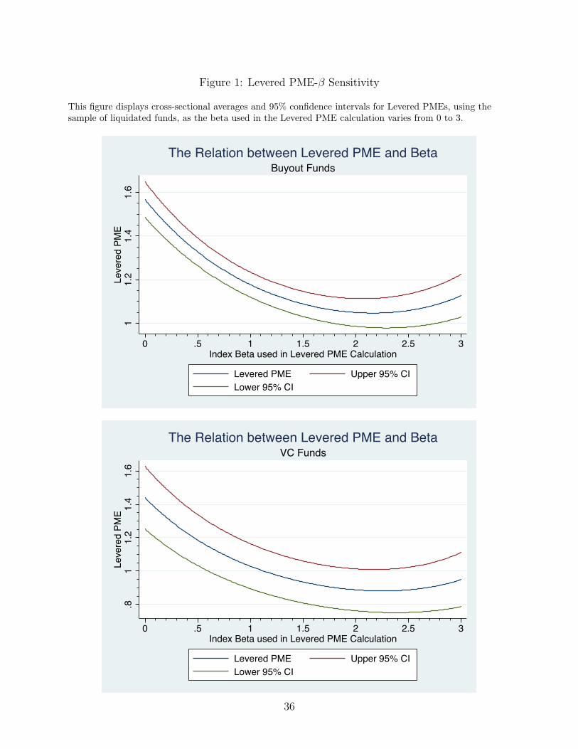
Figure 1: Levered PME-β Sensitivity

This figure displays cross-sectional averages and 95% confidence intervals for Levered PMEs, using thesample of liquidated funds, as the beta used in the Levered PME calculation varies from 0 to 3.

11.

21.

41.

6Le

vere

d PM

E

0 .5 1 1.5 2 2.5 3Index Beta used in Levered PME Calculation

Levered PME Upper 95% CILower 95% CI

Buyout FundsThe Relation between Levered PME and Beta

.81

1.2

1.4

1.6

Leve

red

PME

0 .5 1 1.5 2 2.5 3Index Beta used in Levered PME Calculation

Levered PME Upper 95% CILower 95% CI

VC FundsThe Relation between Levered PME and Beta

36

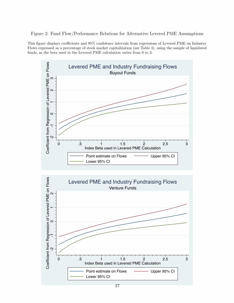
Figure 2: Fund Flow/Performance Relations for Alternative Levered PME Assumptions

This figure displays coefficients and 95% confidence intervals from regressions of Levered PME on IndustryFlows expressed as a percentage of stock market capitalization (see Table 4), using the sample of liquidatedfunds, as the beta used in the Levered PME calculation varies from 0 to 3.

-2-1

01

23

Coe

ffici

ent f

rom

Reg

ress

ion

of L

ever

ed P

ME

on F

low

s

0 .5 1 1.5 2 2.5 3Index Beta used in Levered PME Calculation

Point estimate on Flows Upper 95% CILower 95% CI

Buyout FundsLevered PME and Industry Fundraising Flows

-2-1

01

2C

oeffi

cien

t fro

m R

egre

ssio

n of

Lev

ered

PM

E on

Flo

ws

0 .5 1 1.5 2 2.5 3Index Beta used in Levered PME Calculation

Point estimate on Flows Upper 95% CILower 95% CI

Venture FundsLevered PME and Industry Fundraising Flows

37

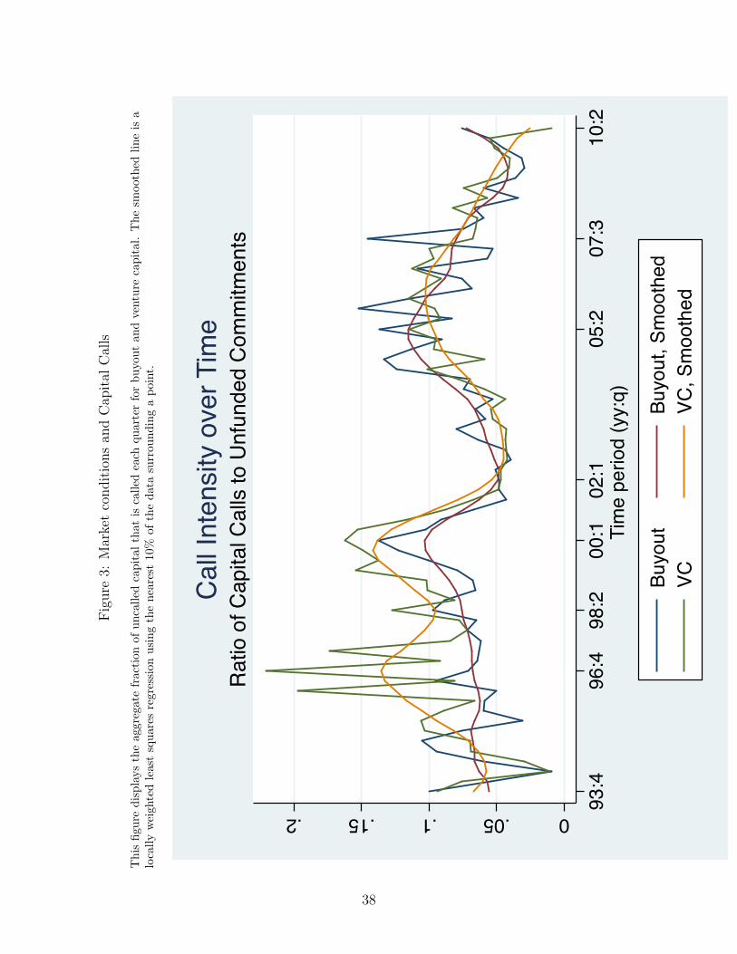
Fig

ure

3:M

arke

tco

ndit

ions

and

Cap

ital

Cal

ls

Thi

sfig

ure

disp

lays

the

aggr

egat

efr

acti

onof

unca

lled

capi

tal

that

isca

lled

each

quar

ter

for

buyo

utan

dve

ntur

eca

pita

l.T

hesm

ooth

edlin

eis

alo

cally

wei

ghte

dle

ast

squa

res

regr

essi

onus

ing

the

near

est

10%

ofth

eda

tasu

rrou

ndin

ga

poin

t.

0.05.1.15.2 93:4

96:4

98:2

00:1

02:1

05:2

07:3

10:2

Tim

e pe

riod

(yy:

q)

Buyo

utBu

yout

, Sm

ooth

edVC

VC, S

moo

thed

Rat

io o

f Cap

ital C

alls

to U

nfun

ded

Com

mitm

ents

Cal

l Int

ensi

ty o

ver T

ime

38

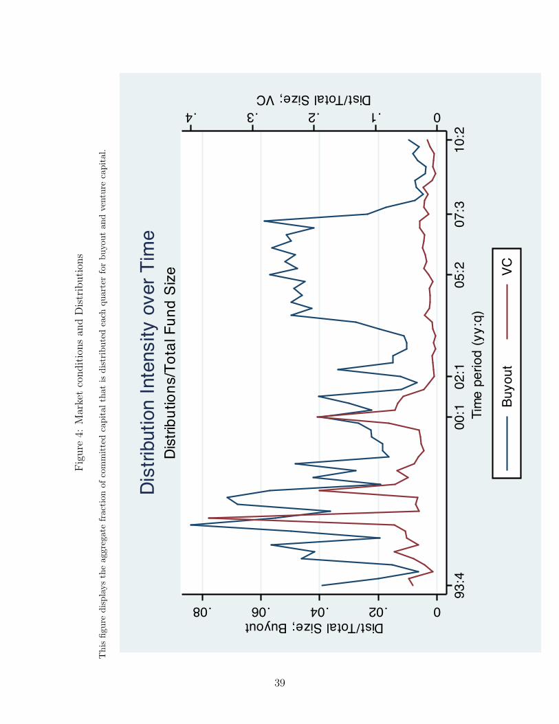
Fig

ure

4:M

arke

tco

ndit

ions

and

Dis

trib

uti

ons

Thi

sfig

ure

disp

lays

the

aggr

egat

efr

acti

onof

com

mit

ted

capi

tal

that

isdi

stri

bute

dea

chqu

arte

rfo

rbu

yout

and

vent

ure

capi

tal.

0.1.2.3.4Dist/Total Size; VC

0.02.04.06.08Dist/Total Size; Buyout

93:4

00:1

02:1

05:2

07:3

10:2

Tim

e pe

riod

(yy:

q)

Buyo

utVC

Dist

ribut

ions

/Tot

al F

und

Size

Dist

ribut

ion

Inte

nsity

ove

r Tim

e

39

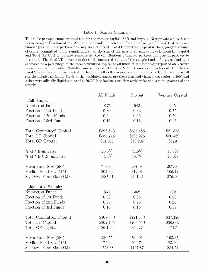
Table 1: Sample Summary

This table presents summary statistics for the venture capital (VC) and buyout (BO) private equity fundsin our sample. Fraction of 1st, 2nd, and 3rd funds indicates the fraction of sample funds of that sequencenumber (position in a partnership’s sequence of funds). Total Committed Capital is the aggregate amountof capital committed to our sample funds (i.e. the sum of the sizes of all sample funds). Total LP Capitaland Total GP Capital indicate, respectively, the contributions of limited partners and general partners tothis total. The % of VE universe is the total committed capital of the sample funds of a given fund typeexpressed as a percentage of the total committed capital to all funds of the same type reported on VentureEconomics over the entire 1984-2009 sample period. The % of VE U.S. universe includes only U.S. funds.Fund Size is the committed capital of the fund. All dollar amounts are in millions of US dollars. The fullsample includes all funds. Funds in the liquidated sample are those that had vintage years prior to 2006 andeither were officially liquidated as of 6/30/2010 or had no cash flow activity for the last six quarters of thesample.

All Funds Buyout Venture CapitalFull Sample:

Number of Funds 837 542 295Fraction of 1st Funds 0.30 0.32 0.25Fraction of 2nd Funds 0.24 0.23 0.26Fraction of 3rd Funds 0.16 0.16 0.15

Total Committed Capital $596,843 $535,485 $61,358Total LP Capital $585,745 $525,276 $60,469Total GP Capital $11,088 $10,209 $879

% of VE universe 26.5% 41.6% 10.8%% of VE U.S. universe 34.4% 55.7% 15.9%

Mean Fund Size ($M) 713.06 987.98 207.96Median Fund Size ($M) 204.34 312.91 106.12St. Dev. Fund Size ($M) 1887.61 2291.21 276.26

Liquidated Sample:Number of Funds 560 368 192Fraction of 1st Funds 0.33 0.35 0.28Fraction of 2nd Funds 0.23 0.23 0.23Fraction of 3rd Funds 0.16 0.15 0.18

Total Committed Capital $308,309 $271,183 $37,126Total LP Capital $302,165 $265,556 $36,609Total GP Capital $6,144 $5,627 $517

Mean Fund Size ($M) 550.55 736.91 193.37Median Fund Size ($M) 172.90 266.72 83.46St. Dev. Fund Size ($M) 1228.38 1467.87 284.51

40

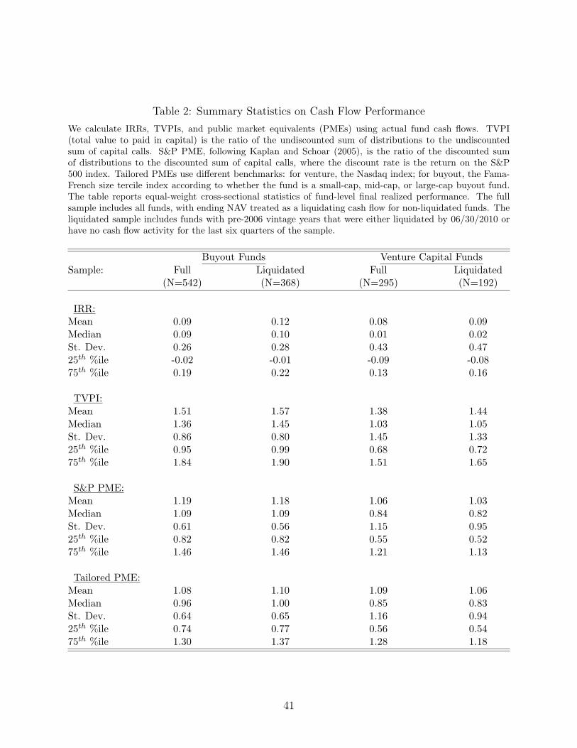
Table 2: Summary Statistics on Cash Flow Performance

We calculate IRRs, TVPIs, and public market equivalents (PMEs) using actual fund cash flows. TVPI(total value to paid in capital) is the ratio of the undiscounted sum of distributions to the undiscountedsum of capital calls. S&P PME, following Kaplan and Schoar (2005), is the ratio of the discounted sumof distributions to the discounted sum of capital calls, where the discount rate is the return on the S&P500 index. Tailored PMEs use different benchmarks: for venture, the Nasdaq index; for buyout, the Fama-French size tercile index according to whether the fund is a small-cap, mid-cap, or large-cap buyout fund.The table reports equal-weight cross-sectional statistics of fund-level final realized performance. The fullsample includes all funds, with ending NAV treated as a liquidating cash flow for non-liquidated funds. Theliquidated sample includes funds with pre-2006 vintage years that were either liquidated by 06/30/2010 orhave no cash flow activity for the last six quarters of the sample.

Buyout Funds Venture Capital FundsSample: Full Liquidated Full Liquidated

(N=542) (N=368) (N=295) (N=192)

IRR:Mean 0.09 0.12 0.08 0.09Median 0.09 0.10 0.01 0.02St. Dev. 0.26 0.28 0.43 0.4725th %ile -0.02 -0.01 -0.09 -0.0875th %ile 0.19 0.22 0.13 0.16

TVPI:Mean 1.51 1.57 1.38 1.44Median 1.36 1.45 1.03 1.05St. Dev. 0.86 0.80 1.45 1.3325th %ile 0.95 0.99 0.68 0.7275th %ile 1.84 1.90 1.51 1.65

S&P PME:Mean 1.19 1.18 1.06 1.03Median 1.09 1.09 0.84 0.82St. Dev. 0.61 0.56 1.15 0.9525th %ile 0.82 0.82 0.55 0.5275th %ile 1.46 1.46 1.21 1.13

Tailored PME:Mean 1.08 1.10 1.09 1.06Median 0.96 1.00 0.85 0.83St. Dev. 0.64 0.65 1.16 0.9425th %ile 0.74 0.77 0.56 0.5475th %ile 1.30 1.37 1.28 1.18

41

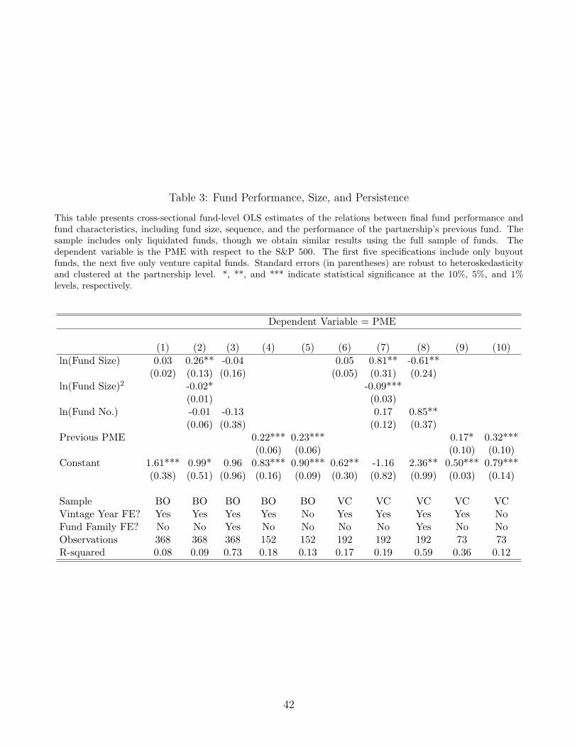
Table 3: Fund Performance, Size, and Persistence

This table presents cross-sectional fund-level OLS estimates of the relations between final fund performance andfund characteristics, including fund size, sequence, and the performance of the partnership’s previous fund. Thesample includes only liquidated funds, though we obtain similar results using the full sample of funds. Thedependent variable is the PME with respect to the S&P 500. The first five specifications include only buyoutfunds, the next five only venture capital funds. Standard errors (in parentheses) are robust to heteroskedasticityand clustered at the partnership level. *, **, and *** indicate statistical significance at the 10%, 5%, and 1%levels, respectively.

Dependent Variable = PME

(1) (2) (3) (4) (5) (6) (7) (8) (9) (10)ln(Fund Size) 0.03 0.26** -0.04 0.05 0.81** -0.61**

(0.02) (0.13) (0.16) (0.05) (0.31) (0.24)ln(Fund Size)2 -0.02* -0.09***

(0.01) (0.03)ln(Fund No.) -0.01 -0.13 0.17 0.85**

(0.06) (0.38) (0.12) (0.37)Previous PME 0.22*** 0.23*** 0.17* 0.32***

(0.06) (0.06) (0.10) (0.10)Constant 1.61*** 0.99* 0.96 0.83*** 0.90*** 0.62** -1.16 2.36** 0.50*** 0.79***

(0.38) (0.51) (0.96) (0.16) (0.09) (0.30) (0.82) (0.99) (0.03) (0.14)

Sample BO BO BO BO BO VC VC VC VC VCVintage Year FE? Yes Yes Yes Yes No Yes Yes Yes Yes NoFund Family FE? No No Yes No No No No Yes No NoObservations 368 368 368 152 152 192 192 192 73 73R-squared 0.08 0.09 0.73 0.18 0.13 0.17 0.19 0.59 0.36 0.12

42

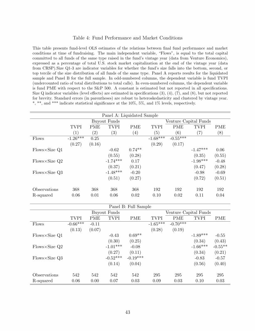
Table 4: Fund Performance and Market Conditions

This table presents fund-level OLS estimates of the relations between final fund performance and marketconditions at time of fundraising. The main independent variable, “Flows”, is equal to the total capitalcommitted to all funds of the same type raised in the fund’s vintage year (data from Venture Economics),expressed as a percentage of total U.S. stock market capitalization at the end of the vintage year (datafrom CRSP).Size Q1-3 are indicator variables for whether the fund’s size falls into the bottom, second, ortop tercile of the size distribution of all funds of the same type. Panel A reports results for the liquidatedsample and Panel B for the full sample. In odd-numbered columns, the dependent variable is fund TVPI(undercounted ratio of total distributions to total calls). In even-numbered columns, the dependent variableis fund PME with respect to the S&P 500. A constant is estimated but not reported in all specifications.Size Q indicator variables (level effects) are estimated in specifications (3), (4), (7), and (8), but not reportedfor brevity. Standard errors (in parentheses) are robust to heteroskedasticity and clustered by vintage year.*, **, and *** indicate statistical significance at the 10%, 5%, and 1% levels, respectively.

Panel A: Liquidated SampleBuyout Funds Venture Capital Funds

TVPI PME TVPI PME TVPI PME TVPI PME(1) (2) (3) (4) (5) (6) (7) (8)

Flows -1.26*** 0.25 -1.68*** -0.55***(0.27) (0.16) (0.29) (0.17)

Flows×Size Q1 -0.62 0.74** -1.47*** 0.06(0.55) (0.28) (0.35) (0.55)

Flows×Size Q2 -1.74*** 0.17 -1.98*** -0.48(0.37) (0.21) (0.47) (0.28)

Flows×Size Q3 -1.48*** -0.20 -0.98 -0.69(0.51) (0.27) (0.72) (0.51)

Observations 368 368 368 368 192 192 192 192R-squared 0.06 0.01 0.06 0.02 0.10 0.02 0.11 0.04

Panel B: Full SampleBuyout Funds Venture Capital Funds

TVPI PME TVPI PME TVPI PME TVPI PMEFlows -0.66*** -0.11 -1.65*** -0.70***

(0.13) (0.07) (0.28) (0.19)Flows×Size Q1 -0.43 0.69** -1.89*** -0.55

(0.30) (0.25) (0.34) (0.43)Flows×Size Q2 -1.01*** -0.08 -1.66*** -0.55**

(0.27) (0.11) (0.34) (0.21)Flows×Size Q3 -0.52*** -0.19*** -0.83 -0.57

(0.14) (0.04) (0.56) (0.40)

Observations 542 542 542 542 295 295 295 295R-squared 0.06 0.00 0.07 0.03 0.09 0.03 0.10 0.03

43

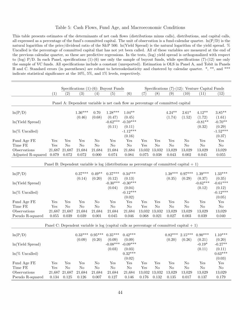
Table 5: Cash Flows, Fund Age, and Macroeconomic Conditions

This table presents estimates of the determinants of net cash flows (distributions minus calls), distributions, and capital calls,all expressed as a percentage of the fund’s committed capital. The unit of observation is a fund-calendar quarter. ln(P/D) is thenatural logarithm of the price/dividend ratio of the S&P 500. ln(Yield Spread) is the natural logarithm of the yield spread. %Uncalled is the percentage of committed capital that has not yet been called. All of these variables are measured at the end ofthe previous calendar quarter, so these are predictive regressions. In the tests, (log) yield spread is orthogonalized with respectto (log) P/D. In each Panel, specifications (1)-(6) use only the sample of buyout funds, while specifications (7)-(12) use onlythe sample of VC funds. All specifications include a constant (unreported). Estimation is OLS in Panel A, and Tobit in PanelsB and C. Standard errors (in parentheses) are robust to heteroskedasticity and clustered by calendar quarter. *, **, and ***indicate statistical significance at the 10%, 5%, and 1% levels, respectively.

Specifications (1)-(6): Buyout Funds Specifications (7)-(12): Venture Capital Funds(1) (2) (3) (4) (5) (6) (7) (8) (9) (10) (11) (12)

Panel A: Dependent variable is net cash flow as percentage of committed capital

ln(P/D) 1.36*** 0.70 1.28*** 1.04** 4.24** 2.61* 4.12** 3.85**(0.46) (0.68) (0.47) (0.45) (1.74) (1.52) (1.72) (1.61)

ln(Yield Spread) -0.62*** -0.59*** -0.81** -0.70**(0.11) (0.11) (0.32) (0.29)

ln(% Uncalled) -1.12*** -1.52***(0.16) (0.37)

Fund Age FE Yes Yes Yes No Yes Yes Yes Yes Yes No Yes YesTime FE Yes No No No No No Yes No No No No NoObservations 21,687 21,687 21,684 21,684 21,684 21,684 13,032 13,032 13,029 13,029 13,029 13,029Adjusted R-squared 0.079 0.072 0.072 0.000 0.074 0.084 0.075 0.038 0.043 0.002 0.045 0.055

Panel B: Dependent variable is log (distributions as percentage of committed capital + 1)

ln(P/D) 0.37*** 0.49** 0.37*** 0.34*** 1.38*** 0.97*** 1.39*** 1.33***(0.14) (0.20) (0.12) (0.13) (0.35) (0.29) (0.37) (0.35)

ln(Yield Spread) -0.30*** -0.30*** -0.62*** -0.61***(0.04) (0.04) (0.12) (0.12)

ln(% Uncalled) -0.12*** -0.12***(0.02) (0.05)

Fund Age FE Yes Yes Yes No Yes Yes Yes Yes Yes No Yes YesTime FE Yes No No No No No Yes No No No No NoObservations 21,687 21,687 21,684 21,684 21,684 21,684 13,032 13,032 13,029 13,029 13,029 13,029Pseudo R-squared 0.055 0.039 0.039 0.001 0.045 0.046 0.068 0.021 0.027 0.003 0.039 0.040

Panel C: Dependent variable is log (capital calls as percentage of committed capital + 1)

ln(P/D) 0.33*** 0.95*** 0.35*** 0.42*** 0.82*** 2.15*** 0.90*** 1.10***(0.09) (0.20) (0.09) (0.09) (0.20) (0.26) (0.21) (0.20)

ln(Yield Spread) -0.08*** -0.09*** -0.19* -0.27**(0.03) (0.03) (0.11) (0.11)

ln(% Uncalled) 0.32*** 0.63***(0.02) (0.03)

Fund Age FE Yes Yes Yes No Yes Yes Yes Yes Yes No Yes YesTime FE Yes No No No No No Yes No No No No NoObservations 21,687 21,687 21,684 21,684 21,684 21,684 13,032 13,032 13,029 13,029 13,029 13,029Pseudo R-squared 0.134 0.125 0.126 0.007 0.127 0.146 0.176 0.132 0.135 0.017 0.137 0.179

44

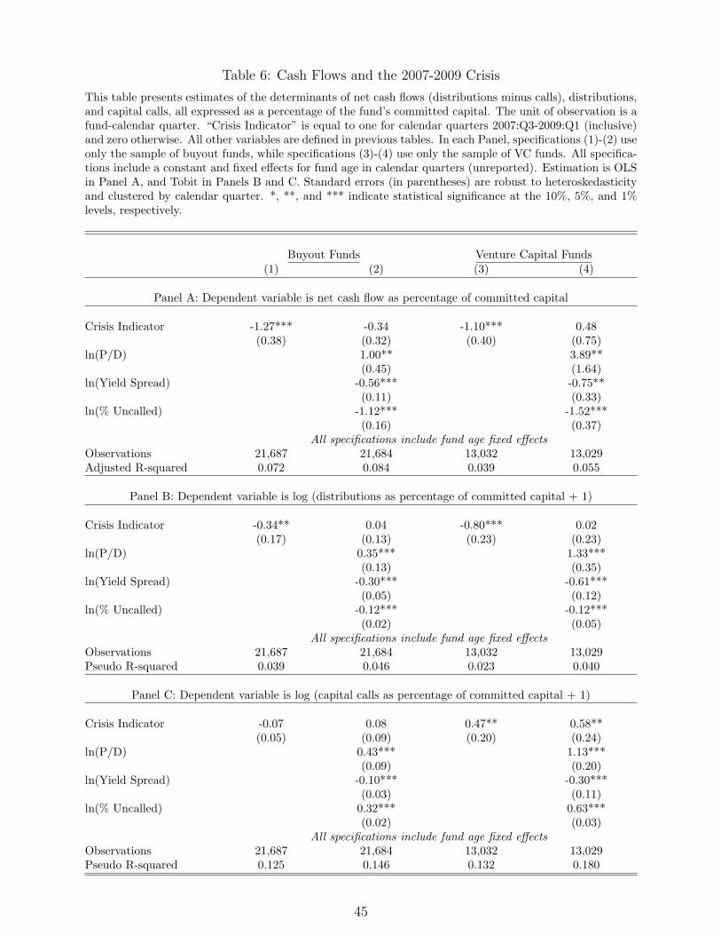
Table 6: Cash Flows and the 2007-2009 Crisis

This table presents estimates of the determinants of net cash flows (distributions minus calls), distributions,and capital calls, all expressed as a percentage of the fund’s committed capital. The unit of observation is afund-calendar quarter. “Crisis Indicator” is equal to one for calendar quarters 2007:Q3-2009:Q1 (inclusive)and zero otherwise. All other variables are defined in previous tables. In each Panel, specifications (1)-(2) useonly the sample of buyout funds, while specifications (3)-(4) use only the sample of VC funds. All specifica-tions include a constant and fixed effects for fund age in calendar quarters (unreported). Estimation is OLSin Panel A, and Tobit in Panels B and C. Standard errors (in parentheses) are robust to heteroskedasticityand clustered by calendar quarter. *, **, and *** indicate statistical significance at the 10%, 5%, and 1%levels, respectively.

Buyout Funds Venture Capital Funds(1) (2) (3) (4)

Panel A: Dependent variable is net cash flow as percentage of committed capital

Crisis Indicator -1.27*** -0.34 -1.10*** 0.48(0.38) (0.32) (0.40) (0.75)

ln(P/D) 1.00** 3.89**(0.45) (1.64)

ln(Yield Spread) -0.56*** -0.75**(0.11) (0.33)

ln(% Uncalled) -1.12*** -1.52***(0.16) (0.37)

All specifications include fund age fixed effectsObservations 21,687 21,684 13,032 13,029Adjusted R-squared 0.072 0.084 0.039 0.055

Panel B: Dependent variable is log (distributions as percentage of committed capital + 1)

Crisis Indicator -0.34** 0.04 -0.80*** 0.02(0.17) (0.13) (0.23) (0.23)

ln(P/D) 0.35*** 1.33***(0.13) (0.35)

ln(Yield Spread) -0.30*** -0.61***(0.05) (0.12)

ln(% Uncalled) -0.12*** -0.12***(0.02) (0.05)

All specifications include fund age fixed effectsObservations 21,687 21,684 13,032 13,029Pseudo R-squared 0.039 0.046 0.023 0.040

Panel C: Dependent variable is log (capital calls as percentage of committed capital + 1)

Crisis Indicator -0.07 0.08 0.47** 0.58**(0.05) (0.09) (0.20) (0.24)

ln(P/D) 0.43*** 1.13***(0.09) (0.20)

ln(Yield Spread) -0.10*** -0.30***(0.03) (0.11)

ln(% Uncalled) 0.32*** 0.63***(0.02) (0.03)

All specifications include fund age fixed effectsObservations 21,687 21,684 13,032 13,029Pseudo R-squared 0.125 0.146 0.132 0.180

45

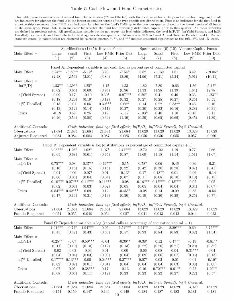
Table 7: Cash Flows and Fund Characteristics

This table presents interactions of several fund characteristics (“Main Effects”) with the focal variables of the prior two tables. Large and Smallare indicators for whether the fund is in the largest or smallest tercile of the type-specific size distribution. First is an indicator for the first fund ina partnership’s sequence. Low PME is an indicator for whether the fund’s PME up to the previous quarter placed in the lowest tercile of all fundsof the same type. Prior Dist. is an indicator for whether the fund had previously distributed capital prior to that quarter. All other variablesare defined in previous tables. All specifications include but do not report the level crisis indicator, the level ln(P/D), ln(Yield Spread), and ln(%Uncalled), a constant, and fixed effects for fund age in calendar quarters. Estimation is OLS in Panel A, and Tobit in Panels B and C. Robuststandard errors (in parentheses) are clustered by calendar quarter. *, **, and *** indicate statistical significance at the 10%, 5%, and 1% levels.

Specifications (1)-(5): Buyout Funds Specifications (6)-(10): Venture Capital FundsMain Effect = Large Small First Low PME Prior Dist. Large Small First Low PME Prior Dist.

(1) (2) (3) (4) (5) (6) (7) (8) (9) (10)

Panel A: Dependent variable is net cash flow as percentage of committed capitalMain Effect 5.94** -5.58** -5.12* 3.23 -7.54* 5.82 -11.39 1.81 3.42 -19.06*

(2.48) (2.56) (2.81) (3.80) (3.89) (4.96) (7.21) (5.24) (5.91) (10.11)Main Effect ×:

ln(P/D) -1.53** 1.39** 1.25* -1.42 1.53 -1.82 2.80 -0.66 -1.36 5.42*(0.62) (0.65) (0.69) (0.95) (0.96) (1.33) (1.98) (1.39) (1.64) (2.78)

ln(Yield Spread) 0.09 0.17 -0.10 0.30* -0.97*** 0.50* 0.41 0.40 0.33 -1.23**(0.18) (0.20) (0.19) (0.17) (0.32) (0.27) (0.28) (0.27) (0.25) (0.55)

ln(% Uncalled) 0.13 -0.01 0.05 0.39*** 0.68* 0.14 0.22 0.33** 0.43 0.16(0.13) (0.12) (0.14) (0.11) (0.37) (0.20) (0.32) (0.16) (0.28) (0.31)

Crisis -0.18 0.59 0.25 0.19 -1.17 -1.03* 0.40 1.10 -0.48 0.11(0.46) (0.54) (0.58) (0.34) (1.19) (0.59) (0.65) (0.69) (0.45) (1.39)

Additional Controls: Crisis indicator, fund age fixed effects, ln(P/D), ln(Yield Spread), ln(% Uncalled)Observations 21,684 21,684 21,684 21,684 21,684 13,029 13,029 13,029 13,029 13,029Adjusted R-squared 0.084 0.084 0.084 0.087 0.085 0.056 0.056 0.055 0.057 0.060

Panel B: Dependent variable is log (distributions as percentage of committed capital + 1)Main Effect 3.93*** -1.26* 1.02* 1.07* 2.41*** -2.72 -1.02 1.19 0.77 2.66

(0.65) (0.68) (0.61) (0.65) (0.87) (1.69) (1.18) (1.14) (1.51) (1.67)Main Effect ×:

ln(P/D) -0.75*** 0.08 -0.37** -0.49*** -0.15 0.78* 0.06 -0.46 -0.36 -0.21(0.16) (0.16) (0.15) (0.16) (0.22) (0.42) (0.30) (0.28) (0.37) (0.41)

ln(Yield Spread) 0.04 -0.06 -0.07* 0.01 -0.13* 0.17 0.18** 0.01 -0.06 -0.14(0.06) (0.06) (0.04) (0.04) (0.07) (0.11) (0.08) (0.10) (0.10) (0.15)

ln(% Uncalled) -0.10*** 0.07*** 0.11*** 0.11*** -0.08 -0.16*** 0.12*** 0.13*** -0.02 0.05(0.02) (0.03) (0.03) (0.02) (0.05) (0.05) (0.04) (0.04) (0.04) (0.07)

Crisis -0.54*** 0.42*** 0.09 0.12 -0.45** -0.08 0.14 -0.09 -0.35 -0.54(0.17) (0.13) (0.21) (0.13) (0.20) (0.19) (0.26) (0.29) (0.25) (0.77)

Additional Controls: Crisis indicator, fund age fixed effects, ln(P/D), ln(Yield Spread), ln(% Uncalled)Observations 21,684 21,684 21,684 21,684 21,684 13,029 13,029 13,029 13,029 13,029Pseudo R-squared 0.054 0.055 0.048 0.054 0.057 0.041 0.043 0.042 0.044 0.053

Panel C: Dependent variable is log (capital calls as percentage of committed capital + 1)Main Effect 1.91*** -0.72* 1.94*** 0.05 2.51*** 2.24** -1.24 -2.29*** 0.60 3.75***

(0.45) (0.42) (0.43) (0.50) (0.57) (0.93) (0.84) (0.89) (0.82) (1.34)Main Effect ×:

ln(P/D) -0.25** -0.07 -0.50*** -0.04 -0.30** -0.38* 0.12 0.47** -0.19 -0.81**(0.11) (0.10) (0.10) (0.12) (0.13) (0.22) (0.20) (0.21) (0.20) (0.32)

ln(Yield Spread) -0.02 -0.03 -0.03 0.01 0.00 -0.06 0.08 0.04 0.31*** 0.04(0.04) (0.04) (0.03) (0.03) (0.04) (0.09) (0.06) (0.07) (0.06) (0.13)

ln(% Uncalled) -0.17*** 0.13*** 0.00 0.04*** -0.27*** -0.07* 0.02 -0.01 -0.01 -0.10*(0.02) (0.02) (0.01) (0.01) (0.04) (0.04) (0.04) (0.03) (0.03) (0.05)

Crisis 0.07 0.05 -0.38*** 0.17 -0.13 0.16 -0.72*** -0.61** -0.22 1.29**(0.08) (0.06) (0.11) (0.12) (0.23) (0.23) (0.22) (0.27) (0.22) (0.57)

Additional Controls: Crisis indicator, fund age fixed effects, ln(P/D), ln(Yield Spread), ln(% Uncalled)Observations 21,684 21,684 21,684 21,684 21,684 13,029 13,029 13,029 13,029 13,029Pseudo R-squared 0.154 0.159 0.147 0.146 0.149 0.184 0.187 0.183 0.181 0.181

46

Appendix

Table A-1 compares coverage and performance statistics for our sample to the samples

available from publicly-available commercial databases Venture Economics (VE), Preqin,

and Cambridge Associates. These data sources provide fund-level IRRs only, and not PMEs

or underlying cash flows. Our source for information on the coverage of these databases is

Harris, Jenkinson, and Stucke (2010), Tables 9 and 12. Table A-1 displays coverage and IRR

statistics by vintage year. See Section II.B for a discussion of these comparisons.

Table A-2 reports average final fund performance by vintage year for our sample of

liquidated funds. Performance is measured three ways: IRR, S&P PME, and Tailored PME.

Following Kaplan and Schoar (2005), performance statistics are size-weighed within vintage

year and fund type.

47

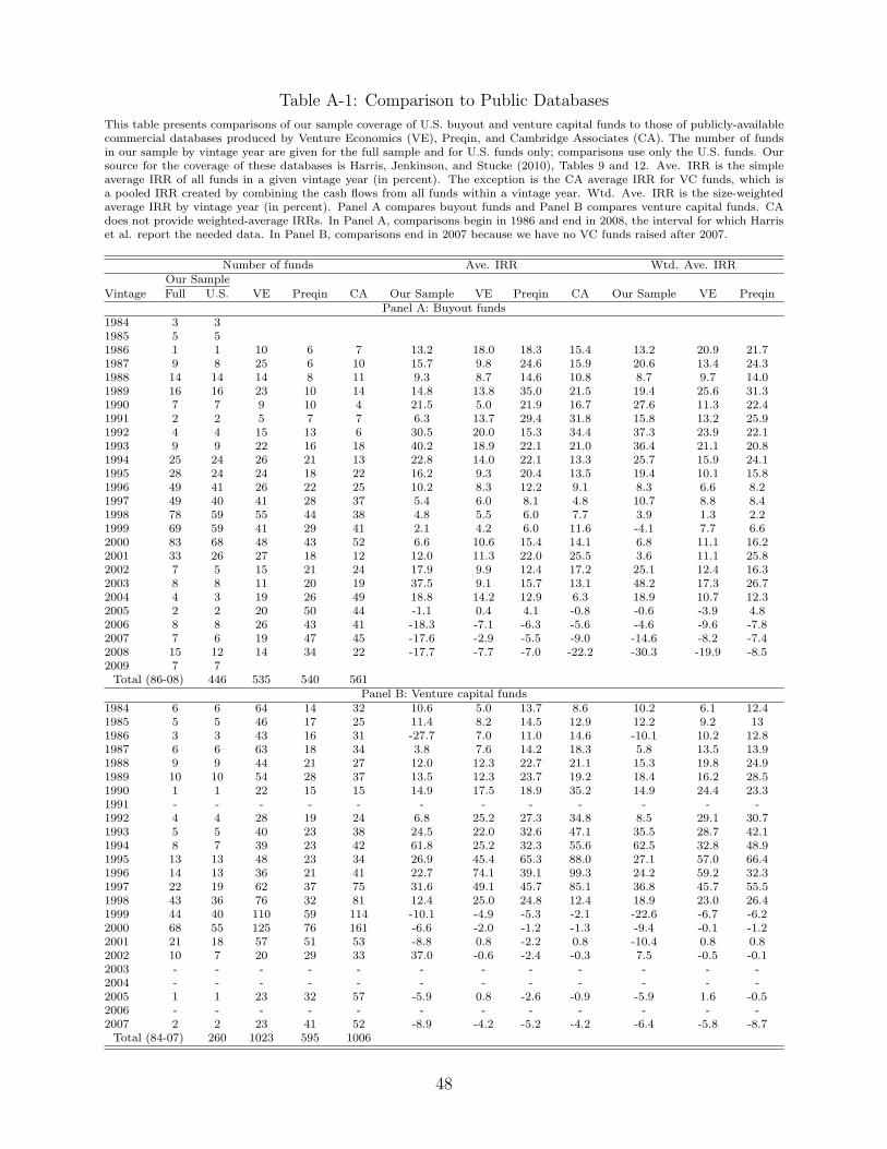
Table A-1: Comparison to Public Databases

This table presents comparisons of our sample coverage of U.S. buyout and venture capital funds to those of publicly-availablecommercial databases produced by Venture Economics (VE), Preqin, and Cambridge Associates (CA). The number of fundsin our sample by vintage year are given for the full sample and for U.S. funds only; comparisons use only the U.S. funds. Oursource for the coverage of these databases is Harris, Jenkinson, and Stucke (2010), Tables 9 and 12. Ave. IRR is the simpleaverage IRR of all funds in a given vintage year (in percent). The exception is the CA average IRR for VC funds, which isa pooled IRR created by combining the cash flows from all funds within a vintage year. Wtd. Ave. IRR is the size-weightedaverage IRR by vintage year (in percent). Panel A compares buyout funds and Panel B compares venture capital funds. CAdoes not provide weighted-average IRRs. In Panel A, comparisons begin in 1986 and end in 2008, the interval for which Harriset al. report the needed data. In Panel B, comparisons end in 2007 because we have no VC funds raised after 2007.

Number of funds Ave. IRR Wtd. Ave. IRROur Sample

Vintage Full U.S. VE Preqin CA Our Sample VE Preqin CA Our Sample VE PreqinPanel A: Buyout funds

1984 3 31985 5 51986 1 1 10 6 7 13.2 18.0 18.3 15.4 13.2 20.9 21.71987 9 8 25 6 10 15.7 9.8 24.6 15.9 20.6 13.4 24.31988 14 14 14 8 11 9.3 8.7 14.6 10.8 8.7 9.7 14.01989 16 16 23 10 14 14.8 13.8 35.0 21.5 19.4 25.6 31.31990 7 7 9 10 4 21.5 5.0 21.9 16.7 27.6 11.3 22.41991 2 2 5 7 7 6.3 13.7 29.4 31.8 15.8 13.2 25.91992 4 4 15 13 6 30.5 20.0 15.3 34.4 37.3 23.9 22.11993 9 9 22 16 18 40.2 18.9 22.1 21.0 36.4 21.1 20.81994 25 24 26 21 13 22.8 14.0 22.1 13.3 25.7 15.9 24.11995 28 24 24 18 22 16.2 9.3 20.4 13.5 19.4 10.1 15.81996 49 41 26 22 25 10.2 8.3 12.2 9.1 8.3 6.6 8.21997 49 40 41 28 37 5.4 6.0 8.1 4.8 10.7 8.8 8.41998 78 59 55 44 38 4.8 5.5 6.0 7.7 3.9 1.3 2.21999 69 59 41 29 41 2.1 4.2 6.0 11.6 -4.1 7.7 6.62000 83 68 48 43 52 6.6 10.6 15.4 14.1 6.8 11.1 16.22001 33 26 27 18 12 12.0 11.3 22.0 25.5 3.6 11.1 25.82002 7 5 15 21 24 17.9 9.9 12.4 17.2 25.1 12.4 16.32003 8 8 11 20 19 37.5 9.1 15.7 13.1 48.2 17.3 26.72004 4 3 19 26 49 18.8 14.2 12.9 6.3 18.9 10.7 12.32005 2 2 20 50 44 -1.1 0.4 4.1 -0.8 -0.6 -3.9 4.82006 8 8 26 43 41 -18.3 -7.1 -6.3 -5.6 -4.6 -9.6 -7.82007 7 6 19 47 45 -17.6 -2.9 -5.5 -9.0 -14.6 -8.2 -7.42008 15 12 14 34 22 -17.7 -7.7 -7.0 -22.2 -30.3 -19.9 -8.52009 7 7

Total (86-08) 446 535 540 561Panel B: Venture capital funds

1984 6 6 64 14 32 10.6 5.0 13.7 8.6 10.2 6.1 12.41985 5 5 46 17 25 11.4 8.2 14.5 12.9 12.2 9.2 131986 3 3 43 16 31 -27.7 7.0 11.0 14.6 -10.1 10.2 12.81987 6 6 63 18 34 3.8 7.6 14.2 18.3 5.8 13.5 13.91988 9 9 44 21 27 12.0 12.3 22.7 21.1 15.3 19.8 24.91989 10 10 54 28 37 13.5 12.3 23.7 19.2 18.4 16.2 28.51990 1 1 22 15 15 14.9 17.5 18.9 35.2 14.9 24.4 23.31991 - - - - - - - - - - - -1992 4 4 28 19 24 6.8 25.2 27.3 34.8 8.5 29.1 30.71993 5 5 40 23 38 24.5 22.0 32.6 47.1 35.5 28.7 42.11994 8 7 39 23 42 61.8 25.2 32.3 55.6 62.5 32.8 48.91995 13 13 48 23 34 26.9 45.4 65.3 88.0 27.1 57.0 66.41996 14 13 36 21 41 22.7 74.1 39.1 99.3 24.2 59.2 32.31997 22 19 62 37 75 31.6 49.1 45.7 85.1 36.8 45.7 55.51998 43 36 76 32 81 12.4 25.0 24.8 12.4 18.9 23.0 26.41999 44 40 110 59 114 -10.1 -4.9 -5.3 -2.1 -22.6 -6.7 -6.22000 68 55 125 76 161 -6.6 -2.0 -1.2 -1.3 -9.4 -0.1 -1.22001 21 18 57 51 53 -8.8 0.8 -2.2 0.8 -10.4 0.8 0.82002 10 7 20 29 33 37.0 -0.6 -2.4 -0.3 7.5 -0.5 -0.12003 - - - - - - - - - - - -2004 - - - - - - - - - - - -2005 1 1 23 32 57 -5.9 0.8 -2.6 -0.9 -5.9 1.6 -0.52006 - - - - - - - - - - - -2007 2 2 23 41 52 -8.9 -4.2 -5.2 -4.2 -6.4 -5.8 -8.7

Total (84-07) 260 1023 595 1006

48

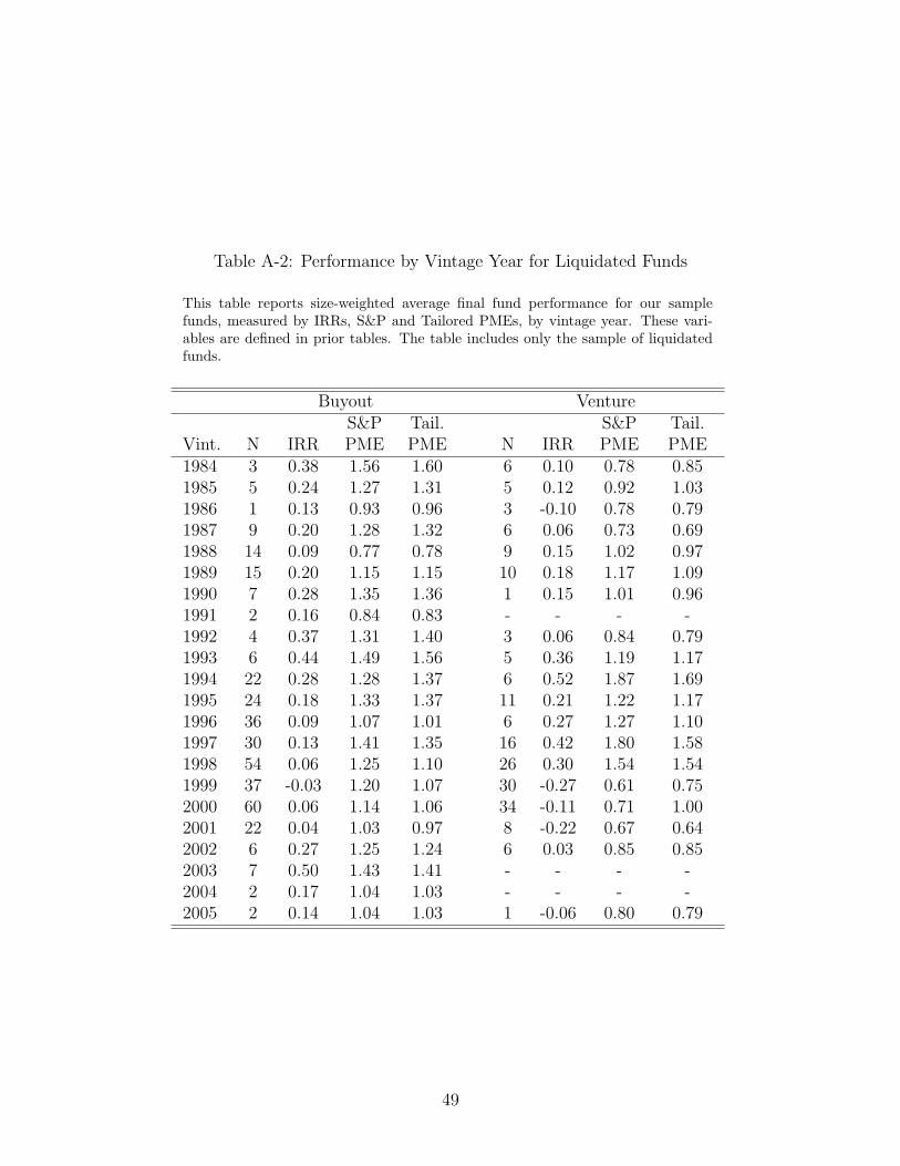
Table A-2: Performance by Vintage Year for Liquidated Funds

This table reports size-weighted average final fund performance for our samplefunds, measured by IRRs, S&P and Tailored PMEs, by vintage year. These vari-ables are defined in prior tables. The table includes only the sample of liquidatedfunds.

Buyout VentureS&P Tail. S&P Tail.

Vint. N IRR PME PME N IRR PME PME1984 3 0.38 1.56 1.60 6 0.10 0.78 0.851985 5 0.24 1.27 1.31 5 0.12 0.92 1.031986 1 0.13 0.93 0.96 3 -0.10 0.78 0.791987 9 0.20 1.28 1.32 6 0.06 0.73 0.691988 14 0.09 0.77 0.78 9 0.15 1.02 0.971989 15 0.20 1.15 1.15 10 0.18 1.17 1.091990 7 0.28 1.35 1.36 1 0.15 1.01 0.961991 2 0.16 0.84 0.83 - - - -1992 4 0.37 1.31 1.40 3 0.06 0.84 0.791993 6 0.44 1.49 1.56 5 0.36 1.19 1.171994 22 0.28 1.28 1.37 6 0.52 1.87 1.691995 24 0.18 1.33 1.37 11 0.21 1.22 1.171996 36 0.09 1.07 1.01 6 0.27 1.27 1.101997 30 0.13 1.41 1.35 16 0.42 1.80 1.581998 54 0.06 1.25 1.10 26 0.30 1.54 1.541999 37 -0.03 1.20 1.07 30 -0.27 0.61 0.752000 60 0.06 1.14 1.06 34 -0.11 0.71 1.002001 22 0.04 1.03 0.97 8 -0.22 0.67 0.642002 6 0.27 1.25 1.24 6 0.03 0.85 0.852003 7 0.50 1.43 1.41 - - - -2004 2 0.17 1.04 1.03 - - - -2005 2 0.14 1.04 1.03 1 -0.06 0.80 0.79

49