Cyclotron waves in a non-neutral plasma columnDaniel H. E. Dubin Citation: Phys. Plasmas 20, 042120 (2013); doi: 10.1063/1.4802101 View online: http://dx.doi.org/10.1063/1.4802101 View Table of Contents: http://pop.aip.org/resource/1/PHPAEN/v20/i4 Published by the American Institute of Physics. Additional information on Phys. PlasmasJournal Homepage: http://pop.aip.org/ Journal Information: http://pop.aip.org/about/about_the_journal Top downloads: http://pop.aip.org/features/most_downloaded Information for Authors: http://pop.aip.org/authors

Cyclotron waves in a non-neutral plasma column

Daniel H. E. DubinDepartment of Physics, University of California at San Diego, La Jolla, California 92093, USA

(Received 22 February 2013; accepted 4 April 2013; published online 25 April 2013)

A kinetic theory of linear electrostatic plasma waves with frequencies near the cyclotron frequency

Xcsof a given plasma species s is developed for a multispecies non-neutral plasma column with

general radial density and electric field profiles. Terms in the perturbed distribution function up to

Oð1=X2csÞ are kept, as are the effects of finite cyclotron radius rc up to Oðr2

c Þ. At this order, the

equilibrium distribution is not Maxwellian if the plasma temperature or rotation frequency is not

uniform. For rc ! 0, the theory reproduces cold-fluid theory and predicts surface cyclotron waves

propagating azimuthally. For finite rc, the wave equation predicts that the surface wave couples to

radially and azimuthally propagating Bernstein waves, at locations where the wave frequency

equals the local upper hybrid frequency. The equation also predicts a second set of Bernstein

waves that do not couple to the surface wave, and therefore have no effect on the external

potential. The wave equation is solved both numerically and analytically in the WKB

approximation, and analytic dispersion relations for the waves are obtained. The theory predicts

that both types of Bernstein wave are damped at resonances, which are locations where the

Doppler-shifted wave frequency matches the local cyclotron frequency as seen in the rotating

frame. VC 2013 AIP Publishing LLC. [http://dx.doi.org/10.1063/1.4802101]

I. INTRODUCTION

This paper considers linear plasma waves near the cy-

clotron frequencies of a multispecies ion plasma column

with near-Maxwellian velocity distributions. We focus on

the z-independent component of the plasma response in the

electrostatic (non-relativistic) limit, in order to simplify the

analysis and make connections to experimental systems that

measure this component. A broad range of devices use the

electrical signal induced by this plasma response in order to

diagnose the charge to mass ratio and/or the relative concen-

tration of plasma species1 (via the technique of “ion-

cyclotron mass spectrometry”). While most of these devices

work in the low-density regime where plasma effects are

small, cyclotron frequency shifts universally arise from elec-

tric fields that can originate either from the plasma or poten-

tials applied to electrodes, as will be discussed here.

Previous papers2,3 have described theory of the electro-

static plasma response near the cyclotron frequency, in the

low temperature “cold-fluid” limit, where thermal effects are

not included. It was found that the cold fluid plasma response

is peaked at frequencies associated with surface cyclotron

waves–electrostatic plasma waves that propagate azimu-

thally along the surface of the plasma column as

expði‘h� ixtÞ, with azimuthal mode number ‘ and fre-

quency x near the cyclotron frequency Xcs¼ qsB=msc for a

given species s. The difference between x and Xcsarises

from a Doppler shift and a Coriolis force effect due to

plasma rotation, and from plasma effects proportional to the

density ns of species s. The frequency x can then be used to

diagnose the plasma rotation frequency, the density of the

species, as well as the cyclotron frequency (which deter-

mines the charge to mass ratio of the species, the main inter-

est in mass spectrometry).

In other work,4–6 effects of finite temperature were also

considered. It was observed that electrostatic Bernstein

waves can be excited in addition to the cold fluid surface

waves. These waves propagate both radially and azimuthally

within the plasma, with frequencies that depend on the cy-

clotron frequency, as well as the plasma density and temper-

ature T, which enters through the cyclotron radius

rc ¼ffiffiffiffiffiffiffiffiffiffiffiT=ms

p=Xcs

. An approximate dispersion relation for

the Bernstein waves was derived in Refs. 5 and 6, based on

WKB analysis.

In this paper, we present a theory of the plasma response

near the cyclotron frequency, which describes both the sur-

face cyclotron waves and the Bernstein waves in the regime

xp=Xcs� 1, where xp is the plasma frequency. A wave

equation for the perturbed plasma potential is derived assum-

ing rc=L � 1 and krc � 1 (where k is the wavenumber of

the response and L is the radial scale length of the equilib-

rium plasma), which includes both the surface cyclotron and

Bernstein waves as solutions. This equation is solved

numerically, as well as through the WKB approximation,

which is valid provided kL � 1, and we extend this WKB

solution through to the regime krc � 1.

The Bernstein waves are reflected at locations where

their frequency equals the plasma’s upper hybrid frequency

and can then set up normal modes inside the plasma column.

We find that the dispersion relation for the Bernstein normal

modes is modified from the qualitative result of Ref. 6 due to

linear mode coupling between these modes and the electro-

static surface cyclotron waves. This coupling also allows the

Bernstein modes to be observed via their effect on the exter-

nal electrostatic potential, which can be picked up using

electrodes. An expression is derived for the electrode signal,

which can exhibit peaks at the Bernstein mode frequencies,

consistent with experiments.5 (Previous theory could not

1070-664X/2013/20(4)/042120/25/$30.00 VC 2013 AIP Publishing LLC20, 042120-1

PHYSICS OF PLASMAS 20, 042120 (2013)

explain this phenomenon.) This effect is similar to the linear

mode coupling between electromagnetic waves and

Bernstein waves that is known to occur at the upper hybrid

resonance in neutral plasmas, of importance to cyclotron

heating and current drive in magnetic fusion applications.7–10

We also find a second set of Bernstein modes that do not

couple to the surface cyclotron waves. These modes are in-

ternal to the plasma, having no effect on the external

potential.

To derive the wave equation, we must first derive sev-

eral new results for the cylindrical plasma equilibrium. First,

in Sec. II, we solve for charged particle motion in the equi-

librium radial electric field of the plasma, keeping finite cy-

clotron radius effects, which are necessary to describe the

finite-temperature Bernstein modes. In so doing, we obtain

finite electric field and finite cyclotron radius corrections to

the particle cyclotron frequency and the drift rotation fre-

quency. Next, in Sec. III, we obtain a closed-form expression

for the collisional quasi-equilibrium velocity distribution of

the rotating plasma, for given density, temperature, and ra-

dial electric field profiles, keeping finite-cyclotron radius

effects. The system evolves to this quasi-equilibrium distri-

bution due to collisions between the plasma charges. The

distribution deviates from Maxwellian due to radial varia-

tions in the plasma rotation frequency and temperature;

eventually on a longer “transport” timescale, these variations

are wiped out by viscosity and thermal conduction, but dur-

ing an intermediate timescale between the collision time and

the transport time, they are present and affect the velocity

distribution.

Next, in Sec. IV, we derive a general dispersion relation

for linear electrostatic waves on this near-Maxwellian quasi-

equilibrium by linearizing and solving the Vlasov equation

with an added Krooks collision operator. The solution is

obtained for general radial density, temperature, and electric

field profiles. In Sec. V, we focus on the plasma response for

z-independent perturbations near the cyclotron frequency of

a given species, deriving the aforementioned wave equation,

which keeps terms to first-order in k2r2c . In Sec. VI, we

review the cold-fluid theory of solutions to this equation (the

rc ! 0 limit), discussing the surface cyclotron waves that

are predicted to appear under various scenarios. In Sec. VII,

we add finite temperature and in Sec. VIII, we consider

WKB solutions to the wave equation. In Sec. IX, we consider

the behavior of the WKB solutions for a few examples.

II. PARTICLE ORBITS

Consider the orbit of a particle with charge 6q and

mass m in a uniform magnetic field 7Bz and a cylindrically

symmetric potential /0ðrÞ. Here, q and B are positive-

definite quantities. For positive (negative) charges, we

assume a magnetic field in the �ðþÞz direction, so that vari-

ous frequencies (cyclotron, drift rotation) are positive for ei-

ther sign of charge; i.e., the resultant circular motions

associated with each frequency are counter-clockwise when

viewed from a location on the z axis above the orbit. The

Hamiltonian for this particle, expressed in cylindrical coordi-

nates ðr; h; zÞ, is

Hðr; pÞ ¼ p2r

2mþ

ph þqB

2cr2

� �2

2mr2þ p2

z

2mþ /0ðrÞ; (1)

where pr ¼ m _r; ph ¼ mr2ð _h � Xc=2Þ; and pz ¼ m _z are the

momenta canonically conjugate to r, h, and z, respectively,

and Xc ¼ qB=mc is the “bare” cyclotron frequency of an iso-

lated particle. Note that /0 has units of potential energy; it is

q times the electrostatic potential. This potential can arise

from voltages applied to cylindrically symmetric electrodes or

from a cylindrically symmetric equilibrium distribution of

plasma charges, which produces a “mean-field” equilibrium

potential. In this case, H is the mean field Hamiltonian for the

motion of a charge in the static field produced by the other

charges. However, /0ðrÞ can also arise from the interaction of

a charge with its own image in the cylindrical electrodes of

the trap, even in the absence of other charges.11 This image

charge potential is typically weak compared to other poten-

tials and is often neglected, but it should be kept in high-

precision work.12 For example, for a point charge q at radius rwithin a hollow cylindrical conductor of radius rw, this image

potential is most easily expressed as an integral:

/image0 ðrÞ ¼ � q2

rw

X1‘¼�1

2

p

ð10

dx I2‘ x

r

rw

� �K‘ðxÞI‘ðxÞ

; (2)

where I‘ and K‘ are modified Bessel functions. Expressions

for the image potential for other electrode geometries, both

cylindrically symmetric and asymmetric, can be found in

Ref. 11.

The Hamiltonian given in Eq. (1) is separable, with three

constants of the motion ph, pz, and H? ¼ H � p2z=2m. We

will find it useful to replace the constant H? by the action

l ¼ 12p

Þprdr, where the line integral is performed along the

closed radial particle orbit. Since pr can be expressed as a

function of H?; ph, and r via Eq. (1), this implies

l ¼ lðH?; phÞ. Inverting this relation yields H? ¼ H?ðl; phÞ,the perpendicular Hamiltonian written in terms of the action.

When the magnetic field is large, this transformation can

be accomplished perturbatively in an expansion in 1/B via

Hamiltonian perturbation theory. This expansion requires

that the cyclotron frequency associated with radial particle

oscillations is large compared to the other motional frequen-

cies, in particular the “drift” frequency associated with hmotion in the radial electric field. As a corollary, this also

requires that the spatial scale length of the electric field, L,

be large compared to the cyclotron radius, so that we can

perform Taylor expansions of the field around the guiding

center position. (This latter requirement is sometimes vio-

lated in cyclotron mass spectrometry, where large amplitude

cyclotron motion can be driven by external fields.) The

result, good to order 1=B4, is

H?ðl;phÞ ¼ lXðr0Þ þ/0ðr0Þ þe2E2ðr0Þ

2mX2c

þ e4E3ðr0Þm2r0X

4c

þ l2e4

8m2X2c

� 15

2

Eðr0Þr3

0

� 15

2

E0ðr0Þr2

0

� 5E00ðr0Þ

r0

� 1

2E000ðr0Þ

� �þOðe6Þ; (3)

042120-2 Daniel H. E. Dubin Phys. Plasmas 20, 042120 (2013)

where e is an ordering parameter used to keep track of the

order in 1/B of different terms, primes denote derivatives

with respect to r, EðrÞ ¼ �@/0=@r, and r0ðphÞ is the radial

location of the effective potential minimum, i.e., the mini-

mum of /0ðrÞ þ ðph þ qBr2=2cÞ2=2mr2, as given by the so-

lution to

R4 ¼ r40 � 4Eðr0Þ r3

0=mX2c ; (4)

where R �ffiffiffiffiffiffiffiffiffiffiffiffiffiffiffiffiffiffiffiffiffiffiffiffiffi�2ph c=ðqBÞ

p, a constant of the motion (the

lowest-order guiding center radius). The shifted cyclotron

frequency Xðr0Þ is given by the (exact) expression

X2ðr0Þ ¼ X2c �

3Eðr0Þmr0

� E0ðr0Þm

: (5)

Note that the action l appearing in Eq. (3) is of order e. In

fact, this equation implies that to lowest order in e,l � e mv2

?=2Xc, the well-known expression for the cyclotron

action. Also, Eq. (5) shows that the cyclotron frequency is

shifted by the radial electric field. In experiments with low

plasma density or even single particles, the shift arises pre-

dominantly from applied trap potentials and/or image charges.

In this paper, we obtain frequency shifts to collective plasma

modes (as well as single particle frequencies), including

plasma effects, applied potentials, and image charges.

The transformation from ðr; pr; h; phÞ to the action-angle

variables ðw; l; �h; phÞ used in Eq. (3) can be carried out with

generating functions Wr and Wh where13

Wh � phh; (6)

Wrðr; l; phÞ �ðr

prðr;H?; phÞ; (7)

and we have used H? ¼ H?ðl; phÞ. These generating func-

tions relate the new and old coordinates via

w ¼ @

@lðWr þWhÞ ¼

@Wr

@lðr; l; phÞ: (8)

Inverting, this yields

r ¼ rðw; l; phÞ � r0 þ drðw; l; phÞ; (9)

where the second form is actually a definition of dr, the devi-

ation of r from r0 due to finite cyclotron radius effects. Also,

we have

�h ¼ @

@phðWr þWhÞ ¼ hþ @Wr

@phðr; l; phÞ; (10)

which we can rearrange as

h ¼ �h þ dhðw; l; phÞ; (11)

where

dhðw; l; phÞ ¼ �@Wr

@phðrðw; l; phÞ; l; phÞ: (12)

Perturbation analysis, described in Appendix A, provides us

with explicit expressions for dr and dh:

dr ¼X1n¼0

enDrnðq; r0; eÞcos nw; (13)

dh ¼X1n¼1

enDhnðq; r0; eÞsin nw: (14)

Here, Drn and Dhn are given as power series in e up to Oðe4Þin Table I, and q2 � 2l=mXc. The parameter q is, to lowest

order in 1/B, the radius of the cyclotron orbit. The coefficient

Dr0 is the radial change in guiding center position due to fi-

nite cyclotron radius effects. Note that for n � 1, both Drn

and Dhn enter dr and dh at OðenÞ.The inverse of these transformations can also be written

as power series in e. In particular, lðr; vr; vhÞ is given by

l ¼ emv2

r þ v2h

2Xc� e2vh

EðrÞX2

c

þ e3

�mv2hðEðrÞ þ 3rE0ðrÞÞ þmv2

r ð3EðrÞ þ rE0ðrÞÞ þ 2rEðrÞ2

4mrX2c

þOðe4Þ: (15)

The Hamiltonian of Eq. (3) implies that the angle varia-

bles �h and w, and the coordinate z evolve in time according

to

dwdt¼ @H?

@l¼ �Xðr0; qÞ; (16)

d�hdt¼ @H?@ph¼ �x0ðr0; pÞ; (17)

dz

dt¼ @H

@pz¼ pz

m; (18)

where the frequencies �X and �x0 are given by the series

expressions

TABLE I. Orbit coefficients in Eqs. (13) and (14).

n Drn

0 34

e2q2

4r0� 15

64e4q4

r30

þ e4q2

mX2c

38

Eðr0Þr2

0

þ 98

E0ðr0Þr0þ 1

4E00ðr0Þ

� �þ Oðe6Þ

1 qþ e2 �q3

8r20

þ qmX2

c

ð34

Eðr0Þr0þ 1

4Eðr0ÞÞ

� �þ Oðe4Þ

2 � q2

4r0þ e2 3

16q4

r30

� e2q2

mX2c

ð18

Eðr0Þr2

0

þ 38

E0 ðr0Þr0þ 1

12E00ðr0ÞÞ

� �þ Oðe4Þ

3 q3

8r20

þ Oðe2Þ

4 � 564

q4

r30

þ Oðe2Þ

n Dhn

1 qr0þ e2 � 1

2q3

r30

þ qr0

Eðr0Þþ3r0E0 ðr0Þ4mr0X

2c

� �þ Oðe4Þ

2 � q2

2r20

þ e2 12

q4

r40

� q2

8r20

3Eðr0Þþ5r0E0 ðr0Þþr20E00 ðr0Þ=3

mr0X2c

� �þ Oðe4Þ

3 q3

3r30

þ Oðe2Þ

4 � q4

4r40

þ Oðe2Þ

042120-3 Daniel H. E. Dubin Phys. Plasmas 20, 042120 (2013)

�Xðr0; qÞ ¼Xðr0Þ

eþ e3q2

8mXc

� 15

2

Eðr0Þr3

0

� 15

2

E0ðr0Þr2

0

� 5E00ðr0Þr0

� 1

2E000ðr0Þ

� �þ Oðe5Þ; (19)

�x0ðr0; qÞ ¼dr0

dph

@H

@r0

����l;pz

¼ exEðr0Þ þe3xEðr0Þ2

Xc� e3q2

4mXcr0

� 3Eðr0Þr2

0

� 3E0ðr0Þr0

� E00ðr0Þ� �

þ Oðe5Þ;

(20)

and where

xEðr0Þ �Eðr0ÞmXcr0

: (21)

The drift rotation frequency �x0 is, to lowest order in

1/B, given by the E� B drift rotation frequency xE in the ra-

dial electric field. The second term in Eq. (20) is a correction

due to centrifugal force, which acts as an extra radial force

that causes an F� B drift in the h-direction. The terms pro-

portional to q2 are finite cyclotron radius corrections to the

rotation rate.

The cyclotron frequency �X also has finite cyclotron ra-

dius corrections. However, when comparing this expression

to previous expressions for the cyclotron frequency in the

presence of an electric field,14 it is important to remember

that here the frequency is derived as the rate of radial oscilla-

tions, which is not the same as the cyclotron rotation rate

with respect to fixed Cartesian axes since the direction of the

radial unit vector varies in time as the particle moves in h.

Thus, single particle resonances can be shifted from the cy-

clotron frequency �X by (multiples of) the rotation frequency

�x0. In fact, when subjected to external fields varying in r, h,

and t as d/ðrÞei‘h�ixt, we will see that particles can absorb

energy resonantly when the applied fields are at the frequen-

cies x ¼ n �X þ ‘�x0 for any integer n. The resonant interac-

tion with n¼ 1 at a frequency near �X is typically the

strongest resonance and is the main effect observed in ion-

cyclotron mass spectrometry for low density systems.

However, for higher densities, there are collective electro-

static plasma waves that can be excited. These collective

excitations are the subject of the next sections.

One type of system for which these frequency formulae

simplify is the harmonic trap where to a good approximation

(and neglecting z dependence, valid for particles moving in

the z¼ 0 plane), /0ðrÞ / r2. Then, the finite cyclotron radius

corrections to �X and �x0 vanish in Eqs. (19) and (20), and

these frequencies are independent of radial position, which

simplifies the analysis. This is one reason why harmonic

traps are often preferred in ion-cyclotron spectrometry appli-

cations. (For a harmonic trap, our frequencies �X and �x0 are

related to the standard harmonic trap frequencies xþ and

x�,15 via the formulae �x0 ¼ x� and �X ¼ xþ � x�.) Of

course, even in traps designed so that the vacuum field is har-

monic, effects such as plasma space charge and image

charges can add anharmonic corrections to /0, necessitating

inclusion of the frequency corrections described by Eqs. (19)

and (20).

III. EVOLUTION OF THE DISTRIBUTION FUNCTION

We assume that the particle distribution f ðr; v; tÞ for a

single species plasma evolves according to the Boltzmann

equation

@f

@tþ v rf þ q

mEþ v� B

c

� � @f

@v¼ Cðf ; f Þ; (22)

where C is the 2 particle Boltzmann collision operator.

We first consider the cylindrically symmetric quasi-

equilibrium distribution predicted by Eq. (22). Neglecting

collisions, the collisionless Boltzmann equation has time-

independent solutions of the general form

f ¼ f0ðl; ph; pzÞ (23)

since l, ph, and pz are constants of the collisionless motion

described by Eq. (1). Any function of these constants of the

motion is a collisionless (Vlasov) equilibrium. However,

when collisions are taken into account, this distribution

evolves on the timescale of the collision rate to a quasi-

equilibrium near-Maxwellian distribution whose dependence

on the constants of motion is determined by the collision op-

erator.16 However, the temperature, density, and rotation rate

of the equilibrium can have arbitrary radial dependence.

[This quasi-equilibrium then proceeds to evolve in time on a

slower “transport” timescale due to radial fluxes driven by

gradients in the plasma rotation frequency and the plasma

temperature, toward a thermal equilibrium state with no such

gradients. We neglect this slow evolution here.] The deriva-

tion of the quasi-equilibrium distribution function is outlined

in Appendix B. Assuming that the temperature gradient is of

order e2 while density and rotation frequency gradients are

of O(1), the quasi-equilibrium is, to Oðe4Þ,

fqeðl; ph; pzÞ ¼NðRÞ

ð2pTðRÞ=mÞ3=2exp �H=TðRÞf

� lXcð1=TlðRÞ � 1=TðRÞÞ þ Oðe4Þg; (24)

where R �ffiffiffiffiffiffiffiffiffiffiffiffiffiffiffiffiffiffiffiffiffiffi�2ph=mXc

p¼

ffiffiffiffiffiffiffiffiffiffiffiffiffiffiffiffiffiffiffiffiffiffiffiffiffiffiffir2 � 2rvh=Xc

pis the lowest-

order guiding center radius [see Eq. (4)], the function N(R) is

related to equilibrium density n(r) and potential /0ðrÞ,

NðRÞ � nðRÞ expf½/0ðRÞ � 1=2mR2e2x2r ðRÞ=TðRÞg; (25)

the cyclotron temperature TlðRÞ is related to the parallel

temperature T(R) through

TlðRÞ � TðRÞ 1þ e2R

2Xc

@xr

@R

� �; (26)

and xrðRÞ is the fluid rotation frequency, defined as

042120-4 Daniel H. E. Dubin Phys. Plasmas 20, 042120 (2013)

r nðrÞxrðrÞ ¼ð

d3v vhfqe: (27)

[Note that in these velocity integrals, r is held fixed, not R.

The expression for fqe given in Eq. (B25), while less elegant

than Eq. (24), is easier to integrate over velocities.]

Performing the velocity integrals yields the following

expression for xr up to Oðe3Þ:

xrðrÞ ¼e

mXcr� 1

n

@

@rðTðrÞnðrÞÞ þ EðrÞ

� þ e3

� x2r

Xc� T

2mX2cr

r

n

@n

@rþ 3

� �@xr

@r� T

2mX2c

@2xr

@r2

" #

þOðe5Þ: (28)

The lowest order fluid rotation frequency in Eq. (28) is the

familiar expression for diamagnetic and E� B drifts.17 The

Oðe3Þ corrections are due to centrifugal force (the first term)

and thermally averaged finite cyclotron radius corrections

due to shear in the fluid rotation (the 2nd and 3rd terms).

Although xr appears on both sides of this expression, to

Oðe3Þ one can use the lowest-order drift expression for xr on

the right hand side to obtain an explicit expression for xr in

terms of density, potential, and temperature.

When T and xr are uniform (independent of r), Eq. (24)

reduces to the thermal-equilibrium form

fqe ¼N0

ð2pT=mÞ3=2e�H=Tþxrph=T ; (29)

where N0 is a constant. This can be seen by noting that,

when xr and T are constant, Eqs. (25) and (28) imply that

� T

mXcRN

@N

@R¼ xr; (30)

which implies that in thermal equilibrium, NðRÞ ¼ N0exrph=T .

When applied to Eq. (24), this leads to Eq. (29).

However, when T and/or xr are not uniform, Eq. (24) is

not a Maxwellian distribution due to the dependence of R on

vh. Collisions drive the system “as close to a Maxwellian as

possible” when variations in xr and T are present. The non-

Maxwellian nature of fqe is responsible for the difference

between cyclotron temperature Tl and parallel temperature

T. With the definition of Tl given by Eq. (26), the mean ki-

netic energy per particle in each degree of freedom, as deter-

mined by velocity integration over fqe, is given by

hmv2r i ¼ TðrÞ 1þ e2r

2Xc

@xr

@rþ Oðe4Þ

� �; (31)

hmðvh � xrrÞ2i ¼ TðrÞ 1� e2r

2Xc

@xr

@rþ Oðe4Þ

� �; (32)

andhmv2

z i ¼ TðrÞ: (33)

Thus, the mean transverse thermal energy h1=4 mðv2r

þðvh � xrrÞ2Þi is equal to the mean parallel thermal energy

hmv2z=2i. This is required in quasi-equilibrium; otherwise there

will be equipartition of parallel and perpendicular thermal

energy on a collisional timescale. (Note that the differences in

mean radial, axial, and azimuthal thermal energy could, in

principle, be observed using, say, laser doppler diagnostics.)

IV. GENERAL DISPERSION RELATION FOR LINEARWAVES

We now consider small perturbations dfsðr; v; tÞ of

fsðr; v; tÞ away from the quasi-equilibrium fqesgiven by Eq.

(24). Here, we re-introduce a species label s for species with

mass ms and charge qs. The perturbations are described by

linearization of the multispecies version of the Boltzmann

equation, Eq. (22). For simplicity, we use a simple Krook

collision operator of the form C ¼ ��ðfs � fqesÞ. Substituting

fs ¼ fqesþ dfsðr; v; tÞ (34)

and

/ ¼ /0ðrÞ þ dUðr; tÞ (35)

into Eq. (22) and linearizing, we obtain

d

dtdfs þ �dfs ¼

@fqes

@l@dU@wþ @fqes

@ph

@dU

@�hþ @fqes

@pz

@dU@z

; (36)

where

d

dt¼ @

@tþ v r þ EðrÞ

mr � v� zXcs

� � @@v

(37)

is a derivative taken along the orbit of the Hamiltonian of

Eq. (1). The right-hand side of Eq. (36) is written in terms of

action-angle variables.

Next, we Fourier analyze df and dU in h, z, and t, writ-

ing these functions as

dfsðr; v; tÞ ¼ dFsðr; vÞ ei‘hþikzz�ixt (38)

and

dUðr; tÞ ¼ d/ðrÞ ei‘hþikzz�ixt: (39)

Applying Eqs. (9) and (11), we define

d/ðr0 þ drÞ ei‘dh �X1

n¼�1D/‘nðph; lÞ einw; (40)

where the D/‘n are the Fourier coefficients of the left-hand

side, which is periodic in w [see Eqs. (13) and (14)]. We may

then integrate Eq. (36), obtaining

ei‘hþikzz�ixtdFsðr; vr; vh; vzÞ

¼X1

n¼�1D/‘nðph; lÞ in

@fqe

@lþ i‘

@fqe

@phþ ikz

@fqe

@pz

� �

� e��t

ðt�1

dt0 einwðt0Þþi‘�hðt0Þþikzzðt0Þ�iðxþi�Þt0 ; (41)

042120-5 Daniel H. E. Dubin Phys. Plasmas 20, 042120 (2013)

where wðt0Þ; �hðt0Þ, and zðt0Þ are determined by the equations

of motion (16)–(19)

wðt0Þ ¼ w0 þ �Xsðr0; qÞðt0 � tÞ; (42a)

�hðt0Þ ¼ h0 þ �x0sðr0; qÞðt0 � tÞ; (42b)

zðt0Þ ¼ zþ vzðt0 � tÞ: (42c)

Here, the constants of integration w0 and h0 and the constant

of motion l are determined in terms of r, h, vr, and vh by the

conditions

h0 þ dhðw0; r0; qÞ ¼ h; (43)

r0 þ drðw0; r0; qÞ ¼ r; (44)

d _rðw0; r0; qÞ ¼ vr: (45)

Equations (44) and (45) determine w0 and l using Eqs. (4)

and (13), and then Eq. (43) determines h0. Note that no equa-

tion for vh is necessary since vh is determined in terms of rand ph by ph ¼ mvhr � qBr2=2c. Of course, l is also deter-

mined by r, vr , and vh via Eq. (15).

Using Eqs. (42) in Eq. (41), the time integral can be per-

formed, yielding

dFsðr;vr;vh;vzÞ ¼X1

n¼�1e�i‘dhðw0;r0;qÞþinw0D/‘nðph;lÞ

�n@fqes

@lþ ‘@fqes

@phþ kz

@fqes

@pz

n �Xsðr0;qÞþ ‘�x0sðr0;qÞþ kzvz�x� i�

:

(46)

The resonant denominator in Eq. (46) provides an expression

for the frequency x at which there is a strong wave-particle

resonant interaction, as we discussed at the end of Sec. II.

Finally, the dispersion relation for d/ is obtained by

substituting Eqs. (38) and (39) into Poisson’s equation

1

r

@

@rr@d/ðrÞ@r

� ‘2

r2þ k2

z

� �d/ðrÞ

¼ �4pe2X

s

ðd3v dFsðr; vr; vh; vzÞ: (47)

This integro-differential equation for d/ can be solved sub-

ject to the boundary conditions on d/. With regard to Eqs.

(46) and (47), we note that the derivatives with respect to land ph are easiest to evaluate using the form of fqes

given in

Eq. (24), but the velocity integrals are easiest to evaluate

using the equivalent form given in Eq. (B25).

V. CYCLOTRON MODES FOR SPECIES s

We focus on z-independent cyclotron modes, assuming

kz ¼ 0. There are cyclotron modes near multiples n of the cy-

clotron frequency for each species. In this paper, we consider

only the modes for which n¼ 1, near the cyclotron frequency

Xcsof species s, with x ¼ Xcs

þ OðeÞ. Substituting Eq. (24)

[or Eq. (B25)] for fqesinto Eq. (47), expanding the integrand

in e, and carrying out the velocity integrals, we keep enough

terms in the series expressions so that finite temperature cor-

rections to the dispersion relation are obtained. These correc-

tions enter at Oðe2Þ, so, noting that �x0 ¼ OðeÞ and

D/‘n ¼ OðenÞ for n 6¼ 0, analysis of Eq. (47) implies that

terms in the sum over n in dFs can be dropped only for jnj > 2

that fqesmust be evaluated including terms up to Oðe3Þ and

that D/‘n must be evaluated up to Oðe4Þ. The perturbed den-

sity for species s can then be evaluated by performing the ve-

locity integral over dFsðd3vdFs ¼ dnFs

ðrÞ þ dnTsðrÞ; (48)

where dnFsðrÞ is the T¼ 0 “cold fluid” density response to

the perturbed potential d/, and dnTsðrÞ is the T > 0 thermal

correction. The cold fluid density perturbation can also be

derived directly to all orders in e from fluid equations6 and

has the form

4pq2s dnFs

ðrÞ

¼ � ‘r

x2psðrÞ

x

ðXvs � rx0FsðrÞÞd/0ðrÞ þ ‘ðx þ i�Þd/=r

XvsðXvs� rx0Fs

ðrÞÞ � ðx þ i�Þ2

þ 1

xr

@

@rrx2

psðrÞ ‘Xvs

d/=r þ ðx þ i�Þd/0ðrÞXvsðXvs� rx0Fs

ðrÞÞ � ðx þ i�Þ2

" #;

(49)

where x � x� ‘xFsðrÞ is the Doppler-shifted frequency,

Xvs� Xcs

� 2xFs, x2

psðrÞ � 4pq2

s nsðrÞ=ms is the square of

the species s plasma frequency, and xFsðrÞ is the cold-fluid

rotation frequency given by the solution to the equation

2xFsðXcs� xFs

Þ ¼P

s x2psðrÞ. However, the velocity inte-

gral in Eq. (47) yields an expansion in e of this general

expression, including terms of Oðe2Þ:

4pq2s dnFs

ðrÞ ¼ 1

r

@

@rðrðD� 1ÞuðrÞÞ � ðD� 1Þ ‘u

rþ Oðe2Þ;

(50)

where the field amplitude uðrÞ is defined as

uðrÞ � d/0ðrÞ þ ‘d/=r; (51)

DðrÞ � 1� bðrÞaðrÞ (52)

is the dielectric constant for the species s cyclotron modes,

aðrÞ � x� Xcsþ ð2� ‘ÞxE þ rx0EðrÞ=2þ i� (53)

is a frequency “offset”, and

bðrÞ �x2

psðrÞ

2Xcs

(54)

represents the local species density nsðrÞ, expressed as the

equivalent E� B rotation rate for a uniform ns. We do not

display the Oðe2Þ terms in the cold fluid density perturbation

as they are fairly complex and will not be needed in what fol-

lows. The frequency offset a is, in fact, (the negative of) the

042120-6 Daniel H. E. Dubin Phys. Plasmas 20, 042120 (2013)

resonant denominator that appears in Eq. (46) for X¼ 1,

expanded to lowest order in e with the assumption that

x ¼ Xcsþ OðeÞ. This implies that a is also of OðeÞ.

Next, we consider the thermal density correction for

species s, which takes the form

4pq2s dnTs

ðrÞ ¼ �r2c C1 þ

C2

a2þ C3

a3þ C4

a4

� �; (55)

where

C1 ¼ r2‘

bar2‘d/

� �þ 2

‘� 1

r

@

@r� ‘

r

� �b0ua; (56)

C2 ¼x0Er‘ð‘� 1Þ @

@rþ ð‘� 5Þ

r

� bu

þa02‘2 � ‘

r2buþ ‘� 2

rb0u� bu0

r� b0u0 � b00u

�

�a00 2b0uþ bu0 � ð‘� 2Þr

bu

� � a000bu; (57)

C3 ¼ a02 bu0 þ 3b0uþ ð3� ‘Þ bu

r

�

þ 2a0 2a00 � x0E‘ð‘� 1Þ

r

� bu; (58)

C4 ¼ �3a03bu; (59)

where

r2‘ �

1

r

@

@rr@

@r� ‘

2

r2: (60)

Finally, we note that Eq. (49) implies that for a different

species �s 6¼ s with Xc�s � Xcs¼ Oð1=eÞ, dnF�s ¼ Oðe2Þ. Also,

we find the thermal corrections to dn�s are even higher order

in e. We, therefore, neglect dn�s when solving Eq. (47), so

only the density perturbation for species s need be kept for

species s cyclotron waves.

Furthermore, since Eqs. (60) and (51) imply

r2‘d/ ¼ 1

r

@

@rðruÞ � ‘u

r; (61)

the thermal density correction for species s can be written

entirely in terms of u and its derivatives up to third order.

Thus, Eq. (47) combined with Eqs. (48), (50) and (55) con-

stitute a third-order ordinary differential equation (ODE) for

u(r), which must be solved subject to the boundary condi-

tions for d/.

While the ODE is fairly complex, its form can be tested

in various ways. For instance, the thermal corrections, pro-

portional to r2c , enter as expected from analysis for a homo-

geneous system, i.e., dnTs¼ �ns k4r2

cd/=ð2msXcsaÞ.18 Also

for the case ‘ ¼ 1 in a single species plasma, a simple ana-

lytic solution exists6

d/ðrÞ ¼ Ar½xþ i� � Xcsþ xEðrÞ; (62)

due to the fact that this excitation is a center-of-mass oscilla-

tion in which the entire column is displaced, and thermal

effects on the density perturbation must vanish as a conse-

quence. Indeed, substitution of Eq. (51) and (62) into Eq.

(55) for ‘ ¼ 1, along with the Poisson equation relating total

charge density qtot ¼P

s qsns to E� B rotation frequency,

qtotðrÞ ¼B

4pcr

@

@rðr2xEÞ; (63)

yields dnTs ¼ 0 if there is only one species, so that

qtot ¼ qsns. Furthermore, the cold-fluid density perturbation

satisfies r2d/þ 4pq2s dnFs

¼ 0, showing that Eq. (62) is a

solution of Eq. (47) for ‘ ¼ 1 in a single species plasma.

Furthermore, if x is chosen as x ¼ Xcs� xEðrwÞ � i�,

Eq. (62) implies that the perturbed potential at rw vanishes.

This is the frequency of the ‘ ¼ 1 “center of mass” cyclotron

eigenmode in a single species plasma column [correct to OðeÞ].The frequency shift xEðrwÞ is caused by E� B rotation of the

center of mass in the plasma’s image charge electric field.

VI. COLD FLUID THEORY OF SURFACE CYCLOTRONMODES

In the zero-temperature “cold-fluid” limit, the cyclotron

mode dispersion relation becomes

r2d/þ 4pq2s dnFs

¼ 0; (64)

with dnFsgiven by Eq. (50). Following Gould,6 we will solve

this equation for d/ðrÞ using the related field amplitude u(r).

Using Eqs. (50) and (61), Eq. (64) can be written as a first-

order ODE for u(r),6

1

r

@

@rðrDuÞ � ‘

rDu ¼ 0: (65)

The solution of this equation is

uðrÞ ¼ Ar‘�1=DðrÞ; (66)

where the constant A is determined by boundary conditions

on d/ðrÞ. We will consider the following boundary

conditions

d/ðrwÞ ¼ /w; d/ðrinÞ ¼ 0; 0 � rin < rw: (67)

For the special case ‘ � 0 and rin ¼ 0, the 2nd boundary con-

dition must be modified to d/ð0Þ ¼ finite:The first boundary condition corresponds to a potential

of magnitude /w applied to an exterior electrode of radius

rw, oscillating in time at frequency x; and the second bound-

ary condition corresponds to an inner conductor of radius rin

at fixed voltage (see Fig. 1). Taking rin ¼ 0 (by which we

mean no interior conductor) is typical in many experiments.

The equilibrium density of a given species s, nsðrÞ, can

have arbitrary radial dependence, but in most experiments,

xEðrÞ is monotonically decreasing; otherwise, the plasma

can be unstable.26 The E� B rotation frequency is deter-

mined by the total charge density qtot through Eq. (63) (see

Fig. 1). The density of species s need not have the same pro-

file shape as qtotðrÞ since various forces act differently on

different species and can even produce centrifugal or charge

042120-7 Daniel H. E. Dubin Phys. Plasmas 20, 042120 (2013)

separation of the species densities at sufficiently low temper-

ature and large xE.25 We will find that there are surface cy-

clotron waves that propagate along the edge(s) of each

species’ density profile, producing measurable electric fields

at the walls. When there is no inner conductor, there is also a

second set of internal upper hybrid waves that do not affect

the potential outside the plasma.

With the boundary condition d/ðrinÞ ¼ 0, Eq. (51)

implies

d/ðrÞ ¼ r�‘ðrrin

dr0r0‘uðr0Þ: (68)

For the special case rin ¼ 0 (no interior conductor), this must

be modified to

d/ðrÞ ¼ r�‘ Cþðr0

dr0r0‘uðr0Þ

24

35: (69)

For ‘ � 0, the constant C is undetermined, but for ‘ > 0, we

require that C ¼ 0 so that d/ remains finite at r¼ 0.

A. Upper hybrid cutoff

For any ‘, a possible solution of Eq. (65) is Du¼ 0. This

corresponds to a localized upper-hybrid oscillation with

u ¼ Bdðr � rUHÞ, at any location rUH for which DðrUHÞ ¼ 0,

which can be written as aðrUHÞ ¼ bðrUHÞ using Eq. (52). In

the theory of electromagnetic wave propagation, such locations

are referred to as upper hybrid resonances,18 but for the electro-

static Bernstein waves discussed in this paper, these locations

act as cutoffs, reflecting the waves. We, therefore, refer to a

location where a ¼ b as an upper hybrid cutoff. Using Eqs.

(53), (52), and (63), the frequency at cutoff can be written as

xþ i� � Xcs¼ ð‘� 1ÞxEðrUHÞ �

X�s 6¼s

xp�s2ðrUHÞ

2Xcs

: (70)

This is the expression for the upper hybrid frequency in a

rotating plasma column, in the low density limit

xps=Xcs

� 1. At rUH, u(r) is undefined, but it is zero every-

where else.

The potential corresponding to these upper hybrid oscil-

lations is, according to Eq. (69),

d/ ¼ Cr�‘ þ 0; r < rUH

BðrUH=rÞ‘; r > rUH;

(71)

where C¼ 0 if rin > 0 or ‘ > 0. In these instances, the choice

B ¼ /wðrw=rUHÞ‘ matches the boundary conditions at

r ¼ rw, so the oscillation amplitude is clamped by the value

at the wall. But, if rin ¼ 0 and ‘ � 0 either B or C is undeter-

mined, so any oscillation amplitude is allowed; these are sin-

gular upper hybrid eigenmodes. These modes make no

potential outside the plasma; they are internal modes. Note

that these occur only if there is no interior conductor

(rin ¼ 0). Finite temperature effects on these modes will be

discussed in Secs. VII–IX.

B. Surface cyclotron waves for no inner conductor

Turning to the surface cyclotron waves, we first examine

the case where there is no interior conductor. In this case, the

solution domain includes r¼ 0, and then Eq. (66) implies

that nontrivial solutions for u(r) exist only for ‘ � 1. These

waves have angular phase velocity x=‘ � Xcs=‘ in the same

direction as the cyclotron motion. Then, Eq. (66) along with

Eq. (69) implies that

d/ðrÞ ¼ Ar�‘ðr0

dr0r0ð2‘�1Þ

Dðr0Þ ; ‘ > 0: (72)

The constant A is determined by the boundary condition

that d/ðrwÞ ¼ d/w,

A ¼ r‘wd/wðrw

0

dr0r0ð2‘�1Þ=Dðr0Þ

: (73)

A dimensionless measure of the system response to the

applied potential d/w is the admittance function Y, where

Y � rw@d/=@rw

d/w

: (74)

This function is proportional to the surface charge on the

wall electrode for a given wall potential. The out-of-phase

(imaginary) component of Y is due only to the plasma and is

a useful measure of the amplitude of the plasma response to

the applied wall potential. Using Eq. (51), the admittance

can be expressed in terms of d/w and uðrwÞ as

Y ¼ �‘þ rwuðrwÞd/w

;

¼ �‘þ r2‘wðrw

0

dr0r02‘�1=Dðr0Þ: (75)

FIG. 1. Schematic diagram of the charge densities and E� B rotation fre-

quency xE in a non-neutral plasma column consisting of three species.

Cylindrical conductors bound the plasma at rin and rw; in many experiments,

the inner conductor is not present. Centrifugal and/or charge separation25

can cause the species to separate radially, in order of largest to smallest

charge to mass ratio.

042120-8 Daniel H. E. Dubin Phys. Plasmas 20, 042120 (2013)

The imaginary part of the admittance has peaks at frequen-

cies for which the denominator in Eq. (75) is small, i.e.,

where

ðrw

0

dr0 r0ð2‘�1Þ=Dðr0Þ ! 0: (76)

For finite collisional damping and real x, this integral never

equals zero, but for weak damping, minima in its magnitude

approach zero at one or more frequencies corresponding to

the frequencies of weakly damped cyclotron modes in the

cold fluid limit. For the case of a uniform rotation frequency

xE and a uniform density (possibly hollow) plasma column

with outer radius r2 and inner radius r1 (similar to the species

2 profile shown in Fig. 1), the integral in Eq. (76) can be per-

formed analytically. There is a single mode frequency for

each (positive) value of ‘, given by

xþ i� � Xcs¼ ð‘� 2ÞxE þ b 1� r2‘

2 � r2‘1

r2‘w

� �; ‘ � 0:

(77)

The frequency shift ‘xE arises from the Doppler effect due

to plasma rotation. The term �2xE arises from a shift in the

cyclotron frequency caused by the Coriolis force. The term

proportional to b is the frequency shift due to the self-

consistent plasma electric field created by the perturbation.

The shift is reduced by the factor ðr2‘2 � r2‘

1 Þ=r2‘w due to the

effect of image charge electric fields.

For more general density and rotation profiles, the inte-

gral in Eq. (76) must be performed numerically. In the limit

of weak damping, � ! 0, there is a singularity in the inte-

grand at radial locations rUH where DðrÞ ! 0, corresponding

to the aforementioned upper hybrid cutoff. If there is only

one such location, at r ¼ rUH, application of the Plemelj for-

mula to Eq. (72) for � ! 0þ allows one to write the admit-

tance as

Y ¼ �‘þ r2‘w

ðrw

0

Pdr0r0ð2‘�1Þ

Dðr0Þ �pi r2‘�1

UH

jD0ðrUHÞj

24

35:

,(78)

This expression shows that if the density or rotation fre-

quency gradient is large (which makes jD0j large), the

amount of enhanced absorption due to the upper hybrid cut-

off will be small. (This is why no effect of the cutoff appears

in Eq. (77)–the cutoff occurs on the plasma edge, which was

taken to be arbitrarily narrow.) An example with an edge of

finite width is shown in Fig. 2. Here, we plot the imaginary

part of Y versus the applied frequency for a single-species

plasma with a density profile of the form

nðrÞ ¼ n0

2tanh

r2 � r

Dr

� �þ 1

h i; (79)

with associated equilibrium potential (and hence rotation fre-

quency) given by the solution to Poisson’s equation,

r2/0 ¼ �4pq2nðrÞ. Here, and throughout the paper, we

take r2 ¼ rw=2. For this profile, there is a range of

frequencies for which there is a single cutoff. For finite edge

width Dr, even if � ! 0 the peak in Im Y has finite frequency

width caused by energy absorption at the upper hybrid cut-

off. The width in Im Y decreases as Dr decreases (Fig. 3).

Also, as Dr decreases, the location of the peak in the plasma

response approaches the analytic result given by Eq. (77),

shown by the arrow in the figure.

We will see in Secs. VIII and IX that this absorption is

due to the coupling of the surface cyclotron wave to Bernstein

waves. The Bernstein waves draw energy from the surface cy-

clotron wave, causing a broadened frequency response. This

damping mechanism is similar to the absorption of unmagne-

tized surface plasma wave energy that occurs at bulk plasma

resonances in an inhomogeneous unmagnetized plasma.19

C. Surface cyclotron waves for an inner conductorwith radius rin > 0

For the boundary conditions d/ðrinÞ ¼ 0; d/ðrwÞ ¼ /w,

the origin is not in the solution domain and, therefore, Eq.

(66) provides nontrivial surface cyclotron mode solutions for

all integers ‘. Now the perturbed potential is, from Eqs. (68)

and (66),

d/ðrÞ ¼ Ar�‘ðrw

rin

dr0r0ð2‘�1Þ

Dðr0Þ ; (80)

FIG. 2. Imaginary part of the admittance versus frequency for an ‘ ¼ 2 wall

perturbation, in the cold fluid limit, at different collision frequencies �(measured in units of bmax ¼ Max ðbÞ for the density profile of Eq. (79) with

r2 ¼ rw=2;Dr ¼ rw=20, where rw is the wall radius).

FIG. 3. Same as Fig. 2 but for fixed � ¼ bmax=100, at different profile widths

Dr (in units of rw). The arrow shows the frequency for a step profile, Eq. (77).

042120-9 Daniel H. E. Dubin Phys. Plasmas 20, 042120 (2013)

and the constant A is again given by the condition that

d/ðrwÞ ¼ /w. The admittance is then given by Eq. (74)

Y ¼ r2‘wðrw

rin

dr0r0ð2‘�1Þ=Dðr0Þ

� ‘: (81)

Peaks in the admittance function again appear where the de-

nominator approaches zero,

ðrw

rin

dr0r0ð2‘�1Þ

Dðr0Þ ! 0: (82)

For example, for a uniform density hollow column with

inner and outer radii r1 and r2 and with uniform rotation fre-

quency xE, there is again one cyclotron mode per ‘ value, at

frequency

xþ i� � Xcs¼ ð‘� 2ÞxE þ b 1� ðr2=rwÞ2‘ � ðr1=rwÞ2‘

1� ðrin=rwÞ2‘

!:

(83)

For ‘ > 0 and rin ! 0, this formula returns to the previous

result, Eq. (77). However, there are now also modes for

‘ � 0. For example, for ‘ ¼ 0, Eq. (83) reduces to

xþ i� � Xcs¼ �2xE þ b

lnrwr1

rinr2

� �lnðrw=rinÞ

; ‘ ¼ 0: (84)

This is the frequency of a cyclotron “breathing” mode, where

the column oscillates radially without changing its density.

For more general density profiles with an inner conduc-

tor, for which Eq. (83) roughly applies, there are not neces-

sarily any locations where D(r)¼ 0 in the plasma (unlike the

previous example with no inner conductor), so in cold fluid

theory, these modes are then undamped “discrete” eigenmo-

des when � ¼ 0.

An example is shown in Fig. 4 for ‘ ¼ 0 and the same

tanh density profile as we used for Figs. 2 and 3, taking

rin ¼ r1 ¼ 1=10 rw. The potential on the inner conductor is

chosen so that xE is uniform inside the plasma far from the

edges. Now, as � decreases for any fixed value of Dr, peaks

in Im Y become narrower without limit, signifying a discrete

undamped mode in the � ! 0 limit. For small Dr, the peak

in the plasma response occurs at the frequency predicted by

Eq. (84) (the arrow in Fig. 4).

The modes are undamped as � ! 0 in this example

because, for the range of frequencies plotted in Fig. 4, there

is no longer an upper hybrid cutoff, although D changes sign

from a negative value inside the plasma to a positive value

(unity) outside it. This is because D changes sign by passing

through infinity, since aðrÞ ¼ 0 at a location inside the

plasma. This is the location of a wave-particle “resonance”

that has important implications for finite-temperature cyclo-

tron wave propagation.

Because the frequency of the surface cyclotron mode

depends on species density, measurement of the mode

frequency is a useful and nondestructive diagnostic for the

density of each species.2 The internal upper hybrid modes

have frequencies given by Eq. (70), which also depend on

density and rotation frequency, but these modes may be

harder to detect experimentally. There are no peaks in the ad-

mittance function Y, indicating that, within the model of an

infinitely long plasma column, these modes cannot be

observed by their effect on wall image charges. On the other

hand, it should be possible to detect these modes using a

wall electrode located at the end of a finite-length plasma

column.

VII. FINITE TEMPERATURE EFFECTS, BERNSTEINWAVES

When finite temperature terms are added to the analysis

of the surface cyclotron waves, new waves appear, referred

to as Bernstein waves. These waves were analyzed qualita-

tively by Gould.5,6 We will see that these waves couple to

the surface cyclotron waves. Also, when there is no inner

conductor, the ‘ � 0 singular upper hybrid continuum given

by Eq. (70) breaks into another set of finite temperature

Bernstein eigenmodes, which do not couple to the surface

cyclotron waves.

The perturbed potential now satisfies

r2‘d/þ 4pq2ðdnFs

þ dnTsÞ ¼ 0; (85)

where dnFsand dnTs

are given by Eqs. (50) and (55). For

now, we consider only boundary conditions with no inner

conductor where r¼ 0 is included in the domain, and d/ is

specified on the outer wall. We also assume, for now, that

the species s density profile extends to the origin, and that

there is a vacuum region between the plasma and the wall.

Inside the plasma, Eq. (85) is a fourth order homogene-

ous equation for d/, or, alternately, a third order equation

for u when we apply Eq. (61), but outside the equation

reverts to Laplace’s equation, second order in d/ (first order

in u). The general solution of the third order equation for u is

a sum of three independent solutions, u1ðrÞ; u2ðrÞ; u3ðrÞ.

FIG. 4. Imaginary part of the admittance for an ‘ ¼ 0 cold-fluid cyclotron

mode in a plasma with an inner conductor of radius rin ¼ rw=10, for two val-

ues of the profile width Dr (in units of rw) and for �=bmax ¼ 1=20, 1/100 and

1/1000 (in order from broadest to sharpest admittance curves). The arrow

shows the frequency for a step profile, Eq. (84).

042120-10 Daniel H. E. Dubin Phys. Plasmas 20, 042120 (2013)

For ‘ > 0, it can be shown that one of these solutions

(u3, say) blows up at the origin. The interior solution within

the plasma is then

uinðrÞ ¼ B1u1ðrÞ þ B2u2ðrÞ: (86)

This must be matched onto the outer Laplace solution at the

plasma edge. The outer Laplace solution is

uout ¼ Ar‘�1: (87)

The matching of inner and outer solutions is accomplished

by setting

uinðroutÞ ¼ uoutðroutÞ; (88)

where rout is a radius outside the plasma (typically chosen

close to the plasma edge), where Eq. (85) is first-order. A

WKB analysis (Sec. VIII) shows that only one of the two in-

terior solutions remains finite outside the plasma (u1, say);

the other blows up as nðrÞ ! 0. Therefore, we set B2 ¼ 0, so

Eqs. (86)–(88) determine B1 in terms of A,

B1 ¼ A r‘�1out =u1ðroutÞ: (89)

Finally the constant A is determined in terms of the applied

wall potential via Eq. (69),

/w ¼ B1r�‘w

ðrout

0

u1ðrÞr‘dr þ Ar�‘w

ðrw

rout

r2‘�1dr (90)

(taking C¼ 0 since ‘ > 0 is assumed).

Equation (90) determines the amplitude of the plasma

response to the applied wall potential /w. This amplitude is

unbounded wherever the rhs of Eq. (90) equals zero, i.e.,

0 ¼ r‘�1out

ðrout

0

u1ðrÞr‘dr þ u1ðroutÞðrw

rout

r2‘�1dr: (91)

These zeros correspond to a sequence of normal modes–the

aforementioned Bernstein modes. The behavior of these

modes is analyzed in the next sections.

For ‘ � 0, one can show that two of the three interior

solutions blow up at the origin (u2 and u3, say), so

uinðrÞ ¼ B1u1ðrÞ: (92)

This interior solution is not necessarily finite outside the

plasma; it generally blows up as density ns ! 0, so the only

solution is A ¼ B1 ¼ 0, i.e., u¼ 0. Then, Eq. (69) implies

that the solution for d/ is a vacuum potential:

d/ ¼ d/wðr=rwÞ�‘. However, there may be certain choices

of x for which the interior solution does not blow up. These

frequencies correspond to eigenfrequencies of ‘ � 0

Bernstein oscillations.

In the cold-fluid theory, the ‘ � 0 upper hybrid oscilla-

tions were excited over a continuum of frequencies associ-

ated with an upper hybrid cutoff and were localized to a

given radius for a given frequency in the continuum. With

finite temperature, these modes are not localized and may

occur only at discrete frequencies.

VIII. WKB ANALYSIS OF FINITE TEMPERATURECYCLOTRON MODES

The previous general ideas concerning the solution of

Eq. (85) can be illustrated and expanded using a WKB solu-

tion of the problem. We first make some general observa-

tions about the Bernstein wave solutions expected from this

analysis. For a uniform plasma in the low-density regime

xp=Xc � 1, the finite-T dielectric constant DTðx; kÞ near the

cyclotron frequency for species s is18,20

DTðx; kÞ ¼ 1� 2bXcs

xðx� XcsÞ e�k2r2

cI1ðk2r2

c Þk2r2

c

; (93)

where I1ðxÞ is a modified Bessel function. The zeros of the

dielectric constant yield the Bernstein mode dispersion

relation,

xðkÞ ¼ Xcsþ 2b e�k2r2

cI1ðk2r2

c Þk2r2

c

þ O1

X2c

!

¼ Xcsþ bð1� k2r2

c þ…Þ; k rc � 1: (94)

The time-averaged energy density in the waves is

Ew ¼jEj2

16p@

@xðxDTÞ ¼

jEj2

16pXc

x� Xc; (95)

where E ¼ �rd/ is the wave electric field. The energy flux

is

S ¼ vg Ew; (96)

and

vg ¼@x@k¼ �4brc

½k2r2c ðI1 � I0Þ þ 2I1

k3r3c

e�k2r2c k (97)

is the group velocity.

Our wave Eq. (85) should produce results consistent

with the small k limit of these expressions. Outside the

plasma, the solution for u(r) is given by Eq. (87). Inside, we

assume a WKB form

uðrÞ ¼ eSðrÞ; (98)

where we expand the eikonal S(r) in a power series in the cy-

clotron radius rc,

SðrÞ ¼ S0ðrÞrcþ S1ðrÞ þ rcS2ðrÞ þ : (99)

This asymptotic expansion will be useful provided that

rc=L � 1, where L is the scale length of the equilibrium.

The only term in dnTðrÞ that enters the analysis to determine

S0 and S1 is the first term in Eq. (56).

042120-11 Daniel H. E. Dubin Phys. Plasmas 20, 042120 (2013)

Substituting Eqs. (98) and (99) into Eq. (85) and keeping

the lowest order terms in rc yields the following equation

for S0:

D S00 �ba

S030 ¼ 0: (100)

This implies S00 ¼ 0 or S00 ¼ 6ikðrÞrc, where

kðrÞ �ffiffiffiffiffiffiffiffiffiffiffiffiffiffiffiffiffiffiffiffiffiffiffi�aD=ðbr2

c Þq

¼ffiffiffiffiffiffiffiffiffiffiffiffiffiffiffiffi1� a=b

p=rc (101)

is the local radial wavenumber of the solution. For the case

S00 ¼ 0, the solution is slowly varying and is entirely deter-

mined at the next order.

Considering the next-order equation in rc yields the fol-

lowing expression for S1 when S00 ¼ 0:

S01 þD0

D� ð‘� 1Þ

r¼ 0: (102)

The solution is the cold fluid result S1 ¼ �log Dþð‘� 1Þ log r, or

u1ðrÞ ¼r‘�1

DðrÞ : (103)

An order r2c correction to this solution could be found by

working to even higher order, but we will not use that correc-

tion here. This cold fluid solution is invalid if 1/D(r) varies

rapidly, which occurs near the upper hybrid cutoff where

D(r)¼ 0.

The amplitudes of the other two rapidly varying solu-

tions with S00 ¼ 6ikðrÞrc are also obtained by considering

the next-order equation in rc, which now yields

S01ðrÞ þ1

2rþ 1

r

D0

Dþ b0

b� a0

a

� �¼ 0: (104)

Thus, the second and third WKB solutions for u(r) are

u2;3ðrÞ ¼1ffiffirp a

bD

� �14

e6iÐr

kðrÞdr

: (105)

These solutions are traveling waves moving radially

inward or outward, depending on the sign of x and Re(k).

Their wavenumber and amplitude (but not their frequency)

vary in radius as the plasma density and/or rotation rate

varies. The local dispersion relation of these waves follows

from Eq. (101):

a ¼ bð1� k2r2cÞ: (106)

Equation (106) matches the long-wavelength limit of the

Bernstein-mode dispersion relation, Eq. (94), for the shear-

free case; noting that for a rotating system, there is a Doppler

shift to x and a shift to Xc from the Coriolis force that

appears in Eq. (106) through a [see Eq. (53)]. The radial

group velocity follows from the derivative with respect to kof Eq. (106):

vg ¼ �2bkr2c : (107)

The WKB amplitude factor for the Bernstein waves,

u / 1ffiffirp a

bD

� �1=4

; (108)

is consistent with energy conservation. For WKB traveling

waves, the conserved quantity is the total radial energy flux

rS r given by Eq. (96). Identifying x� Xc with a and iden-

tifying jEj2 with u2 [using Eq. (52) and the WKB limit

kr � ‘] implies the following general WKB amplitude

factor:

u / � aðrÞrXcs

vgðr; kÞ

� �1=2

: (109)

To compare this to Eq. (108), we substitute for vg from

Eq. (107), noting that the group velocity can be written as

vg ¼ �2brc

ffiffiffiffiffiffiffiffiffiffiffiffiffiffiffiffi1� a=b

pusing Eq. (106). Substituting this

expression into Eq. (109) and using Eq. (52) yields Eq.

(108), the krc � 1 form of the amplitude factor.

The two WKB solutions in Eq. (105) break down near

r¼ 0; near any upper hybrid cutoffs where DðrÞ ! 0; and

near any “resonances” where aðrÞ ¼ 0 and DðrÞ ! 1, corre-

sponding to strong wave-particle resonant interactions. These

resonances, if they occur, cause damping of Bernstein waves.

Note that the slowly varying “cold fluid” solution u1 also

breaks down at the upper hybrid cutoff, but not at r¼ 0 or at

the a ¼ 0 resonance. Also, when bðrÞ ! 0 at the plasma

edge, Eq. (101) implies that k ! i1, so one Bernstein solu-

tion blows up and the other decays to zero exponentially.

Connection formulae18 must be derived in order to con-

nect WKB solutions on either side of a cutoff or resonance.

We first consider the connection formula for a cutoff.

A. Connection formula for an upper hybrid cutoff

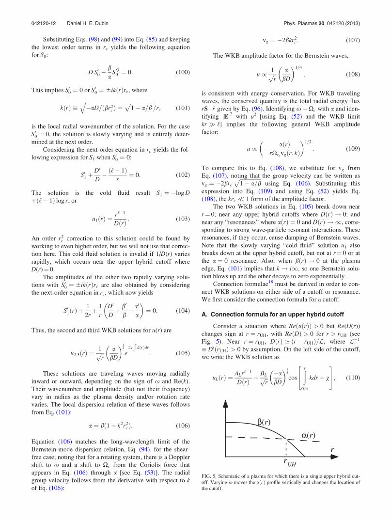
Consider a situation where ReðaðrÞÞ > 0 but Re(D(r))

changes sign at r ¼ rUH, with ReðDÞ > 0 for r > rUH (see

Fig. 5). Near r ¼ rUH, DðrÞ ’ ðr � rUHÞ=L, where L�1

� D0ðrUHÞ > 0 by assumption. On the left side of the cutoff,

we write the WKB solution as

uLðrÞ ¼ALr‘�1

DðrÞ þBLffiffi

rp �a

bD

� �14

cos

ðrrUH

kdr þ v

24

35; (110)

FIG. 5. Schematic of a plasma for which there is a single upper hybrid cut-

off. Varying x moves the aðrÞ profile vertically and changes the location of

the cutoff.

042120-12 Daniel H. E. Dubin Phys. Plasmas 20, 042120 (2013)

where AL and BL are the amplitudes of the solution and v is

the phase. [Throughout the remainder of the paper, we

assume a sign in the square root in Eq. (101) such that

Re k > 0. In this section, we use the krc � 1 form of the

WKB amplitude factor, Eq. (108), since near cutoff k ! 0.]

On the right side of the cutoff, the WKB solution is

uRðrÞ ¼ARr‘�1

DðrÞ þ1ffiffirp a

bD

� �14

BR1e

ÐrrUH

kdr

þ BR2e�Ðr

rUH

kdr

264

375:

(111)

To connect these two solutions, we note that near r ¼ rUH,

Eq. (85) can be approximated as

�r2c u000ðxÞ þ @

@x

x

L u� �

¼ 0; (112)

where x ¼ r � rUH, we have used the relation b=ajr¼rUH¼ 1,

and we have kept only the dominant balance in Eq. (85),

assuming rc=L � 1. [This balance involves only the first

term in dnF (see Eq. (50)) and the first term in Eq. (56).] The

general solution can be written in terms of Airy functions

and integrals of Airy functions:

uðxÞ ¼ D1Aið�xÞ þ D2Bið�xÞ þ D3Cið�xÞ; (113)

where the function Ci is defined as

Cið�xÞ � pAið�xÞð�x�1

dx0Biðx0Þ þ pBið�xÞð1�x

dx0Aiðx0Þ (114)

and �x � x=ðLr2c Þ

1=3. For �x � �1 but jxj=L � 1, we can

connect Eq. (110) to Eq. (113) using the asymptotic form of

Eq. (113). The asymptotic forms of the Airy functions Ai and

Bi are well known.21 The asymptotic forms for Cið�xÞ are

Cið�xÞ ¼1

�xþ 2

�x4þ 40

�x7þ þ

ffiffiffipp

ð��xÞ1=4cos

2

3ð��xÞ3=2 þ p

4

�

� 1þ 385

4608�x3

� �þ 5

48

ffiffiffipp

ð��xÞ7=4sin

2

3ð��xÞ3=2 þ p

4

�

� 1þ 17017

13824�x3þ

� �; �x ��1

Cið�xÞ ¼1

�xþ 2

�x4þ 40

�x7…; �x � 1: (115)

Using the �x � �1 asymptotic form in Eq. (113) along with

the corresponding forms for the Airy functions yields the fol-

lowing lowest-order form for u:

lim�x!�1

uðxÞ ¼ 1ffiffiffippð��xÞ1=4

D1sin2

3ð��xÞ3=2 þ p

4

� ��

þ ðD2 þ pD3Þ cos2

3ð��xÞ3=2 þ p

4

� �þ D3

�x:

(116)

Comparing Eq. (116) to Eq. (110), and noting that for

0�ðrUH�rÞ=L�1, we can approximate 23j�xj3=2 ¼

Ð rUH

r kdr,

DðrÞ¼ x=L, and ð�a=ðbDÞÞ1=4¼ð�L=xÞ1=4, so we obtain

AL ¼ D3r1�‘UH ðr2

c=L2Þ1=3; (117)

BL cos v ¼ffiffiffiffiffiffiffirUH

2p

rðrc=LÞ1=6½D1 þ D2 þ pD3; (118)

BL sin v ¼ffiffiffiffiffiffiffirUH

2p

rðrc=LÞ1=6½D1 � D2 � pD3: (119)

On the right side of the cutoff the lowest order asymptotic

form of Eq. (113) is

lim�x!1

uðxÞ ¼ 1ffiffiffipp

�x1=4

1

2e�2�x3=2=3D1 þ D2e2�x3=2=3

� þ D3=�x:

(120)

Connecting to Eq. (111) for �x � 1 but ðr � rUHÞ=L � 1

implies

AR ¼ D3r1�‘UH ðrc=LÞ2=3; (121)

BR1¼

ffiffiffiffiffiffiffirUH

p

rðrc=LÞ1=6D2; (122)

BR2¼

ffiffiffiffiffiffiffirUH

p

rðrc=LÞ1=6 D1

2: (123)

Eliminating D1, D2, and D3 from Eqs. (117)–(119) and

(121)–(123) yields the connection formulae at an upper

hybrid cutoff,

AL ¼ AR; (124)

BL cos v ¼ BR1ffiffiffi2p þ

ffiffiffi2p

BR2þ

ffiffiffiffiffiffipL2rc

sr‘�1=2UH AR; (125)

BL sin v ¼ �BR1ffiffiffi2p þ

ffiffiffi2p

BR2�

ffiffiffiffiffiffipL2rc

sr‘�1=2UH AR: (126)

These formulae indicate that, at a cutoff, the slowly varying

“cold fluid” solution, responsible for surface cyclotron

waves, and proportional to coefficients AR and AL, is mixed

with the rapidly varying “Bernstein” solutions, proportional

to BR and BL.

B. Behavior near a resonance

There may be locations in the plasma where aðrÞ ¼ 0,

due to shears in the E� B rotation frequency. At such loca-

tions, the WKB Bernstein mode solutions, Eq. (105), are

invalid. This is because Eq. (101) implies that krc ¼ 1 at

a ¼ 0, which breaks the assumption used to derive Eq. (85)

that krc � 1. Therefore, we modify the Bernstein WKB sol-

utions by using the exact Bernstein mode dispersion relation

for a uniform system, Eq. (94), writing the dispersion rela-

tion as

aðrÞ ¼ 2bðrÞ e�k2r2c

I1ðk2r2c Þ

k2r2c

(127)

in order to account for Doppler and Coriolis force shifts due

to plasma rotation. This WKB dispersion relation agrees

042120-13 Daniel H. E. Dubin Phys. Plasmas 20, 042120 (2013)

with the xp=Xc � 1 limit of the Bernstein dispersion rela-

tion for a rotating uniform density single species plasma col-

umn, derived in Ref. 22. This equation shows that at a

resonance, the radial wavenumber k approaches infinity, not

1=rc as our approximate dispersion relation, Eq. (106),

predicted.

Furthermore, the resonance does not act as a turning

point for rays, unlike the upper hybrid cutoff. The rays are

curves in the ðr; krÞ plane describing the trajectory of

Bernstein wave packets. The rays are obtained from Eq.

(127), as contours of constant x.23 When aðrÞ and bðrÞ have

the form shown in Fig. 6, these constant x contours have the

form shown schematically in Fig. 7(a). The rays are simply

diverted to large k without reflecting, as opposed to the case

of a upper hybrid cutoff (Fig. 5), for which the rays have a

turning point (Fig. 7(b)).

Furthermore, the WKB wave amplitude becomes large

at the resonance. As krc !1, Eq. (127) implies that

aðrÞ !ffiffiffi2

p

rbðrÞk3r3

c

; (128)

so the radial group velocity approaches zero as

vg ! �3

ffiffiffi2

p

rbðrÞk4r3

c

: (129)

Using these equations in the expression for conservation of

energy flux, Eq. (96) implies that, near the resonance where

a! 0,

jEj2 / 1

½aðrÞ1=3: (130)

These large amplitude large k Bernstein waves will be

absorbed by the plasma at the resonance. The absorption

mechanism could be viscous damping due to large k, nonlin-

ear processes due to large amplitude such as wave-breaking,

or direct Landau damping at the resonance. [None of these

effects are included in Eq. (85), which does not apply at a

resonance.] Such damping is observed in experiments on

fusion plasmas.10

Since the Bernstein waves are absorbed at a resonance

rather than being reflected, there are generally no longer any

Bernstein normal modes in WKB theory, since normal

modes are standing waves that require interference between

waves propagating radially in both directions. However, a

reflection is still possible if there is an abrupt density change

in the plasma with kL < 1, which violates the WKB approxi-

mation. This case has been considered by Spencer et al. for

‘ ¼ 0 modes.24

On the other hand, the cold fluid solution to Eq. (85)

passes through the resonance, essentially unchanged. In cold

fluid theory, we have already observed that the solution for

u(r), Eq. (66), merely changes sign at locations where

aðrÞ ¼ 0. When finite temperature corrections are added, we

find that this is still the case provided that rc=L � 1. To

derive this result, we expand aðrÞ near the resonance, writing

a ¼ x0

rRðr � rRÞ; (131)

where

x0 � rR@a@r

����r¼rR

: (132)

Defining f � ðx0=rRÞu=a and x � r � rR, so that u¼ xf,the dominant balance for jx=rRj � 1 and rc=jrRj � 1 in Eq.

(85) is

FIG. 6. Schematic of a plasma with parameters chosen so that there is a sin-

gle resonance.

FIG. 7. (a) Rays (contours of constant x)

for Bernstein waves at a frequency corre-

sponding to the aðrÞ profile in Fig. 6. (b)

Analogous ray (contour of constant x)

for Bernstein waves at a frequency corre-

sponding to the aðrÞ profile in Fig. 5.

042120-14 Daniel H. E. Dubin Phys. Plasmas 20, 042120 (2013)

r2c f 000 þ @

@x

f 0

x

� �� �þ f 0 ¼ 0: (133)

[This dominant balance involves the first term in Eqs. (50),

(56), and (58), and Eq. (59).] The solution is

f ¼ D1J0

x

rc

� �þ D2Y0

x

rc

� �þ D3: (134)

The Bessel functions J0 and Y0 are the two Bernstein

wave solutions near resonance, but with an incorrect (finite)

wavelength due to the aforementioned breakdown of Eq.

(85) as krc becomes of order unity. However, the fluid solu-

tion to Eq. (85) remains valid provided that it remains slowly

varying. In fact, for small rc, Eq. (134) shows this to be true:

near resonance the fluid solution for f is simply the constant

D3, which implies that u ¼ D3 aðrÞ. This solution can be

asymptotically matched onto the fluid solution away from

the resonance, Eq. (66), via the choice D3 ¼ �Ar‘�1R =bðrRÞ.

Thus, the fluid solution is unaffected by the resonance

even when finite temperature effects are included (provided

that rc is small). This is illustrated in Fig. 8, which displays a

solution of Eq. (85) for a single-species plasma with the den-

sity profile of Eq. (79) and for ‘ ¼ 0. For this ‘ value, there is

a range of frequencies for which a single resonance occurs.

The figure shows uðrÞ for one such frequency and for

rc ¼ rw=100, compared to the fluid solution; the two solutions

are matched at r ¼ 0:6rw. A small collision frequency � is

added to the frequency in order to regularize the poles in Eq.

(85) that occur at the resonance; but the results displayed are

in the limit of small �. One can see that for small but finite rc,

the fluid solution closely follows the numerical solution.

IX. WKB SOLUTIONS: EXAMPLES

The connection formulae derived in Sec. VIII B can be

used to solve for the potential response of a finite-

temperature plasma to an oscillatory wall signal. The behav-

ior of the solutions is influenced by the locations of cutoffs

and resonances. We consider several examples.

A. One upper-hybrid cutoff

The simplest example is the case of a single upper-

hybrid cutoff. For instance, this can occur for the lightest

species in a multi-component plasma with nearly uniform

total density that has undergone some centrifugal separation;

see Fig. 1.25 In this case, aðrÞ is nearly constant over the

range of radii for which bðrÞ is nonzero, and there is a range

of mode frequencies for which

0 < a < Max ðbÞ: (135)

There is then a single cutoff at the radial location rUH where

aðrUHÞ ¼ bðrUHÞ (see Fig. 5). For frequencies outside this

range, the real part of the dielectric constant D(r) does not

change sign and the plasma response is well-represented by

the fluid limit, Eq. (66). This fluid response was already dis-

cussed in Sec. V.

For frequencies within the range given by Eq. (135), the

upper hybrid cutoff causes reflection of the Bernstein waves

that sets up a strong resonant plasma response at a discrete

set of mode frequencies. Inside the plasma, to the left of the

cutoff, DðrÞ < 0 and a > 0, so the WKB solution for u(r) is

of the form given by Eq. (110)

u ¼ ALr‘�1

DðrÞ þ BL �2rca

rvgðr; kÞ

� �1=2

� cos

ðrrUH

kðrÞdr þ v

0@

1A; r < rUH: (136)

Here, we have used the general form for the WKB amplitude

factor, Eq. (109), normalized so as to approach the krc � 1

form, Eq. (108), as krc becomes small. The phase v is deter-

mined by the r < rUH form of the solution near r¼ 0. For

r=Dr � 1, we can take nðrÞ � n0 and then the solution of

Eq. (85) that is finite at r¼ 0 is

uðrÞ ¼ ALr‘�1

DðrÞ þ E J‘�1ðk0rÞ; r

L � 1; (137)

where k0 ¼ kð0Þ, and J‘ðxÞ is a Bessel function. This solution

can be connected to Eq. (136) for r=rc � 1 using the large

argument form of the Bessel function.21 This implies

v ¼ðrUH

0

kðrÞdr � ð‘� 1Þ p2� p

4: (138)

To complete the solution for u, we match Eq. (136) to the

form for r > rUH, using Eqs. (124)–(126) adding the require-

ments that the solution remain finite as nðrÞ ! 0, and the

outer solution match to Eq. (87). This implies that the coeffi-

cient BR1 must vanish, so the matching conditions are

AL ¼ A; (139)

BL cos v ¼ffiffiffi2p

BR2 þ

ffiffiffiffiffiffipL2rc

sr�1=2UH A; (140)

BL sin v ¼ffiffiffi2p

BR2 �

ffiffiffiffiffiffipL2rc

sr�1=2UH A; (141)

where L�1 ¼ D0ðrUHÞ.

FIG. 8. Comparison of cold fluid theory, Eq. (66), to a solution to Eq. (85)

when there is a resonance. Fluid solution and numerical solution are

matched at r=rw ¼ 0:6. The resonance is located at the arrow.

042120-15 Daniel H. E. Dubin Phys. Plasmas 20, 042120 (2013)

Equations (140) and (141) can be used to determine BR2

and BL in terms of A

BL ¼

ffiffiffiffiffiffipLrc

sr‘�1=2UH

cosðvþ p=4ÞA; (142)

BR2 ¼

ffiffiffiffiffiffipLrc

sr‘�1=2UH

2tan vþ p

4

� �L: (143)

Equation (69) then allows determination of the perturbed

potential d/. Near r¼ 0, substitution of Eq. (137) into Eq.

(69) yields

d/ðrÞ ¼ Cr�‘ þ Ar�‘ðr0

dr0r02‘�1

Dðr0Þ þE

k0

J‘ðk0rÞ; r

L � 1;

(144)

where we require C ¼ 0 for ‘ > 0 and A¼ 0 for ‘ � 0. This

can be connected onto the WKB form by using the following

integration identity, obtained using integration by parts:

limrc!0

ðba

dr gðrÞ eiUðrÞ=rc ’ rc

iU0ðrÞ gðrÞ eiUðrÞ=rc

����b

a

þ Oðr2c Þ;

(145)

provided that there are no locations in a � r � b, where

U0ðrÞ ¼ 0. We break Eq. (69) into two terms,

d/ ¼ d/ðNrcÞ þ r�‘ðr

Nrc

dr0 r0‘uðr0Þ; (146)

where N � 1 but Nrc � Dr. This allows use of the WKB

form, Eq. (136) in the integral, and Eq. (144) in the first

term. After asymptotic-expansion of J‘ for large argument,

and cancellation of terms involving N, we obtain

d/ðrÞ ¼ Cr�‘ þ Ar�‘ðr0

dr0r02‘�1

Dðr0Þ þBL

k� 2rca

rvgðk; rÞ

� �1=2

� sin

ðrrUH

kðrÞdr þ v

0@

1A; rc � r < rUH: (147)

This form for d/ is valid to the left of the upper hybrid cut-

off, but away from the origin.

To find d/ to the right of the cutoff, one must integrate

across the cutoff using the connecting form, Eq. (113). We

write Eq. (69) as

d/ðrÞ ¼ d/ðrUH � Na0Þ þ r�‘ðrUHþNa0

rUH�Na0

dr0 r0‘uðr0Þ

þ r�‘ðr

rUHþNa0

dr0r0‘uðr0Þ; (148)

where a0 � ðLr2c Þ

1=3;N � 1 but N a0=L � 1.

We can use the WKB form for d/, Eq. (147), in the first

term. In the last term, we can use u ¼ Ar‘�1=D, and in the

middle term, we can use Eq. (113). Noting that DðrÞ’ L�1ðr � rUHÞ for r near rUH, and using Eq. (107) for vg

near the cutoff where krc ! 0, Eq. (142) for BL, Eqs. (139)

and (117)–(119), we find that terms involving N cancel, and

we are left with

d/ðrÞ ¼ Cr�‘ þ Ar�‘ðr0

Pdr0r0ð2‘�1Þ

Dðr0Þ þ D1a0r‘UHr�‘; (149)

whereÐP means the principal part of the integral, neglecting

the pole at r ¼ rUH. In deriving Eq. (149), we have also used

the identitiesÐ1�1 Aið�xÞ d�x ¼ 1 and limN!1

Ð N�N Cið�xÞ d�x

¼ 0. The latter follows by applyingÐ1�1 d�x to Eq. (114) and

integrating by parts.

Substituting for D1 from the solution of Eqs.

(118)–(119) and using Eq. (142) yields

r‘d/ðrÞ ¼ Cþ A

ðr0

Pdr0r0ð2‘�1Þ

Dðr0Þ þ pL r2‘�1UH tan

�vþ p

4

�24

35;

r � rUH � a0: (150)

For ‘ > 0, C¼ 0 is required, so Eqs. (150), (75), and (51)

determine the admittance

Y ¼ r2‘wðrw

0

Pdr0r0ð2‘�1Þ=Dðr0Þ þ pL r2‘�1UH tan½vþ p=4

� ‘ : (151)

Here, v is given by Eq. (138), and k by Eq. (101) when a=bis close to unity (so that krc � 1). More generally, we can

extend the validity of Eq. (151) to all krc by using Eq. (127)

for k.

The first term in the denominator of Eq. (151) is the

same as for cold fluid theory, Eq. (78). The second term

leads to the Bernstein modes. These modes occur wherever

the denominator vanishes, i.e., where

ðrUH

0

kdr ¼ ð‘� 1Þp2

þ np� arctanr1�2‘

UH

pL

ðrw

0

P dr0r0ð2‘�1Þ

Dðr0Þ

24

35(152)

for any integer n [using Eq. (138)]. This is the dispersion

relation for the ‘ > 0 Bernstein modes in the WKB limit for

a single cutoff.

For a uniform density step profile of radius r2 and

assuming krc � 1, we can estimate the frequency predicted

by Eq. (152) by taking k constant, given by Eq. (101), and

rUH ’ r2, yielding

a ’ b 1� r2c

r22

x2n

� �; (153)

where xn is the right hand side of Eq. (152). Note that in a step

profile, L ! 0 and arctanð1Þ ¼ p=2, so xn ¼ ð‘=2 þnÞp.

042120-16 Daniel H. E. Dubin Phys. Plasmas 20, 042120 (2013)

As mode number n increases, the frequency decreases, with a

frequency spacing between modes proportional to plasma

temperature through the factor r2c=r2

2. (This result is only an

estimate since a step profile has rapid variation that violates

the WKB approximation kL � 1. However, a solution of Eq.

(85) for a step profile does predict Bernstein mode frequencies

of the form given in Eq. (153), albeit with a different value for

xn.)

In Fig. 9, we display the admittance Y for the density

profile given by Eq. (79), versus cyclotron radius rc. The sin-

gularities of Y locate the frequencies of the Bernstein modes.

We assume aðrÞ is uniform and equal to 4 Max ðbÞ=5, and

for Dr ¼ rw=10, r2 ¼ rw=2, and ‘ ¼ 2 using Eq. (101) for k.

Equation (101) is correct only for small krc. We use this

form for k in order to compare to numerical solutions of Eq.

(85) (the dots in Fig. 6), which are valid only for krc � 1.

The WKB form for this function, Eq. (151), is an excellent

fit to the numerical solution of Eq. (85).

In Fig. 10, we show two of the potential eigenfunctions

for these modes, compared to the WKB forms, using the

krc � 1 expressions for the WKB wave number and ampli-

tude in order to better compare to solutions of Eq. (85).

When there is finite damping �, the admittance exhibits a

sequence of peaks at frequencies determined by the solution of

Eq. (152) (see Fig. 11, plotted for ‘ ¼ 1). In this figure, we use

the general form for k, from a solution of Eq. (127) for kða=bÞ,rather than Eq. (101). The solution of Eq. (85) is compared to

the WKB prediction on the right side of the figure, where

krc � 1 for the Bernstein modes. The numerical solution dif-

fers from the WKB solution as a=bmax ! 1 because WKB

theory breaks down as kL becomes small. For sufficiently small

rc, there is a regime for which both krc � 1 and kL � 1,

where the WKB and numerical solutions of Eq. (85) match.

As the cyclotron radius rc decreases, the spacing

between the admittance peaks in Fig. 11, and the height of

the peaks, decreases until the result is indistinguishable from

the cold-fluid admittance given by Eq. (78). This happens

because, in Eq. (138), the imaginary part of v (due to finite

�) becomes large and negative as rc decreases, so that

tanðvþ p=4Þ ! �i, implying that Eq. (151) becomes identi-

cal to Eq. (78). This will occur roughly when �rUH � jvgj

FIG. 9. Admittance versus cyclotron radius at fixed frequency and uniform

aðrÞ profile, a ¼ 4bmax=5, � ¼ 0, and density given by Eq. (79). Dots: nu-

merical solution of Eq. (85). Solid lines: WKB approximation, Eq. (151).

Singularities in Y occur at the frequencies of Bernstein modes.

FIG. 10. Perturbed potential of ‘ ¼ 2 Bernstein modes for two different tem-

peratures but the same frequency, and assuming uniform aðrÞ, with

a ¼ 4bmax=5, and density given by Eq. (79). Solid lines: numerical solution

of Eq. (85). Dashed lines: WKB approximation, Eqs. (147), (150), (138),

(101), and (107). The dashed vertical line shows the location of the upper

hybrid cutoff. (a) rc=rw ¼ 0:014 and (b) rc=rw ¼ 0:008: The WKB approxi-

mation improves for smaller rc, and breaks down as expected near r¼ 0 and

r ¼ rUH.

FIG. 11. Admittance versus frequency for uniform a, density given by Eq.

(79), and � ¼ bmax=40 for ‘ ¼ 1, at three temperatures, with corresponding

cyclotron radii rc measured in units of rw. As rc decreases, the admittance

approaches cold fluid theory, Eq. (70). For larger rc, Bernstein mode peaks are

evident. Curves: WKB theory given by Eq. (151), (138), and (127). Dots: nu-

merical solution of Eq. (85), shown only in the regime of validity for

Bernstein solutions of Eq. (85), krc � 1. The arrow at a=bmax ¼ 0:75 shows

the prediction of Eq. (77) for the frequency of the surface cyclotron wave.

042120-17 Daniel H. E. Dubin Phys. Plasmas 20, 042120 (2013)

[note that jvgj decreases as rc decreases; see Eq. (107)]. In

this regime, the Bernstein modes merge and disappear, and

the cold-fluid limit is valid. Physically, the Bernstein waves

are carrying energy away from the surface cyclotron wave

and then damping due to collisions before normal modes can

be set up.

1. Internal Bernstein modes with ‘£ 0

In addition to the Bernstein modes which occur for

‘ > 0, there is a second set of Bernstein modes with ‘ � 0,

related to the singular upper hybrid modes discussed in Sec.

VI A. When there is no inner conductor, the ‘ � 0 Bernstein

modes are purely internal modes, having no effect on the ad-

mittance. These Bernstein modes satisfy cosðvþ p=4Þ ¼ 0,

which implies v ¼ ðnþ 1=4Þp, for any integer n. Then, Eq.

(142) implies that AL ¼ A ¼ 0 and BL is undetermined.

Outside the plasma, u¼ 0.

Inside the plasma, d/ is given by Eq. (147) with

AL ¼ A ¼ 0. Outside, d/ is given by Eq. (149) with D1 given

in terms of BL by Eqs. (118) and (119). Thus,

d/ðrÞ ¼ Cr�‘ þ

BL

k� 2rca

rvg

� �1=2

sin

ðrrUH

kdr þ ðnþ 1=4Þp

24

35 ; r < rUH

�BL

ffiffiffiffiffiffiffiffiffiffipLrc

rUH

rð�1Þn rUH

r

� �‘; r > rUH:

8>>>>><>>>>>:

(154)

For ‘ � 0, C can be chosen arbitrarily. By taking

C ¼ BL

ffiffiffiffiffiffiffiffiffiffiffiffiffiffiffiffiffiffiffipLrc=rUH

pr‘UHð�1Þn, the perturbed potential out-

side the plasma vanishes. The result is an internal Bernstein

mode with arbitrary amplitude BL. The mode has no effect

on the admittance; it can neither be detected nor launched

using wall potentials. These modes have similar appearance

to the ‘ > 0 Bernstein modes, except that d/ ¼ 0 outside the

plasma. The dispersion relation is given by v ¼ ðnþ 1=4Þp,

which implies, using Eq. (138),

ðrUH

0

kdr ¼ ‘ p2þ np : (155)

The frequencies predicted by Eq. (155) [using the gen-

eral form for kða=bÞ found by solving Eq. (127)] are shown

in Fig. 12 for ‘ ¼ 0 and compared to the frequencies

obtained from numerical solution of Eq. (85), again taking

Eq. (79) as the species s density profile with Dr ¼ 1=10 rw,

and a uniform in r. There is good agreement with Eq. (85)

solutions when krc � 1 (the lowest-order modes), and fre-

quencies show the expected behavior given by Eq. (127) as

wavenumber increases. A few of the low-order modes are

displayed in Fig. 13.

B. Two upper hybrid cutoffs

There are circumstances where the a and b profiles have

the form shown in Fig. 14. For instance, in a centrifugally

separated plasma, the density of a species of intermediate

mass may have the form shown while the overall density is

uniform, so that a is roughly constant;25 see Fig. 1. There is

then a range of frequencies for which there are two upper

hybrid cutoffs, at radii rUH1and rUH2

, rUH1< rUH2

. The

Bernstein dispersion relations are modified by the second

cutoff.

In between the cutoffs, the WKB solution for u(r) can

be written in two equivalent ways,

FIG. 12. Frequency spectrum of internal ‘ ¼ 0 Bernstein modes for two val-

ues of the cyclotron radius (measured in units of rw). Plasma parameters are

chosen, so that there is a single cutoff: the aðrÞ profile is assumed to be uni-

form, and density is given by Eq. (79). Crosses: numerical solution of Eq.

(85), valid for the low order modes with krc � 1. Dots: WKB approxima-

tion, Eq. (155), valid for kL > 1.

FIG. 13. The five lowest order internal Bernstein potential eigenmodes for

‘ ¼ 0 for the same plasma parameters as in Fig. 12, taking rc ¼ 1=60.

042120-18 Daniel H. E. Dubin Phys. Plasmas 20, 042120 (2013)

uðrÞ ¼ Ar‘�1

Dþ

r‘�1=2UH2

cosðv2 þ p=4Þ

"

� � 2pL2arvg

� �1=2

cos

ðrrUH2

kdr þ v2

!#(156)

or

uðrÞ ¼ Ar‘�1

Dþ

r‘�1=2UH1

cosðv1 � p=4Þ

"

� �2pL1arvg

� �1=2

cos

ðrrUH1

kdr þ v1

!#; (157)

where L�11 ¼ jD0ðrUH1

Þj and L�12 ¼ D0ðrUH2

Þ. These solu-

tions must match, and therefore we require that the phases v1

and v2 satisfy

v1 ¼ v2 �ðrUH2

rUH1

k dr; (158)

and also

cosðv2 þ p=4Þ ¼ rUH2

rUH1

� �‘�1=2ffiffiffiffiffiffiL2

L1

scosðv1 � p=4Þ : (159)

The perturbed potential then follows from Eq. (69). We

must now integrate over the intermediate form, Eq. (113), at

both rUH1and rUH2

, to obtain the following WKB result for

d/ðrÞ:

d/ ¼ Cr�‘ þ Ar�‘ðr0

Pdr0r02‘�1

Dðr0Þ þ A

0 ; r < rUH1

�pL1r2‘�1UH1

tan v1 �p4

� �r�‘ þ

r‘�1=2UH1

kcos v1 �p4

� �

� �2pL1arvg

� �1=2

cos

ðr

rUH1

kdr þ v1

!; rUH1

< r < rUH2

p L2r2‘�1UH2

tan v2 þp4

� �� L1r2‘�1

UH1tan v1 �

p4

� �h ir�‘; r > rUH2

:

8>>>>>>>>>>><>>>>>>>>>>>:

(160)

The Bernstein modes with ‘ > 0 have C¼ 0 and satisfy

d/ðrwÞ ¼ 0, which implies the WKB dispersion relation

ðrw

0

Pdr0r02‘�1

Dðr0Þþp L2r2‘�1UH2

tan

�v2þ

p4

��L1r2‘�1

UH1tan

�v1�

p4

��

¼0: (161)

The Bernstein modes with ‘ � 0 have C 6¼ 0 and satisfy

A¼ 0 and cosðv1 � p=4Þ ¼ 0 ¼ cosðv2 þ p=4Þ [but

A=cosðv1 � p=4Þ finite], which by Eq. (158) requires

ðrUH2

rUH1

k dr ¼ ðn� 1=2Þp (162)

for any integer n.

C. Admittance regimes for the ‘> 0 cyclotronresponse in a single-species plasma

For a single species plasma with a monotonically

decreasing density profile, the driven response to a wall

potential with given mode number ‘ at a real frequency near

the cyclotron frequency exhibits several regimes that depend

on the locations of cutoffs and resonances. These in turn

depend on the a and b profiles.

For ‘ � 0, the only possible plasma excitations are in-

ternal Bernstein modes (unless there is an inner conductor

as in Sec. VI C). Furthermore, the aðrÞ profile for ‘ � 0 has

the form shown in Fig. 15(b): it is monotonically decreasing

in r. A cutoff, if one occurs, now traps the modes on the

outside of the plasma. In this case, there will also generally

be a resonance which will cause strong absorption unless

the plasma edge is sharp compared to k, so that a reflection

at the edge can occur. In any case, the ‘ � 0 excitations

have no effect on the admittance because they are internal

modes.

For ‘ > 1, the aðrÞ profile has a typical form shown in

Fig. 15(b); it may be non-monotonic, depending on the

sharpness of the edge in the density profile, and the value of

‘. Cutoffs and resonances occur in various locations depend-

ing on the frequency and mode number.

For ‘ > 1, the different regimes are

FIG. 14. a and b profiles for a case with two upper hybrid cutoffs.

042120-19 Daniel H. E. Dubin Phys. Plasmas 20, 042120 (2013)

1. x 2 Xc > ð‘2 1Þbmax or x 2 Xc < ð‘2 1ÞxE ðrw Þ: Fluidregime

In this regime there are no resonances or cutoffs, so

the admittance should be nearly that of a cold fluid plasma

(Sec. IV); see Eq. (75).

2. ð‘2 2Þbmax 1 Da < x 2 Xc < ð‘2 1Þbmax : Bernsteinmode regime

Here, Da is the depth of the minimum in aðrÞ (if a mini-

mum exists–see Fig. 15(b)). In this regime, there is a single

upper hybrid cutoff, so the admittance is as described in Sec.

IX A: it displays peaks at the Bernstein mode frequencies,

whose widths vanish as collisional damping � vanishes; see

Eq. (151).

3. ð‘2 1ÞxE ðrw Þ< x 2 Xc < ð‘2 2Þbmax 1 Da: Resonanceregime

In this regime there are one or possibly two resonances,

along with a cutoff at larger radius. At the cutoff, the cold

fluid solution (driven by the wall potential) couples to a

Bernstein wave. This wave then carries energy to the nearest

resonance, where it is absorbed via one of the processes

mentioned in Sec. VIII B. Thus, the solution for u(r) to the

right of the cutoff is Eq. (66), and to the left (but away from

the resonance) it is

u ¼ Ar‘�1

Dþ B

�2rcarvg

� �1=2

eiÐ r

rUHkdr: (163)

Here, the positive sign in the exponential is chosen because

the group velocity, given by Eq. (107), will then be negative,

carrying energy to smaller radii according to Eq. (96).

Furthermore, the coefficients B and A are related by the con-

nection formulae (124)–(126) where, comparing Eq. (163)

(calculated near the cutoff where krc ! 0) to (110), we find

BL cos v ¼ B;

BL sin v ¼ �iB;

AL ¼ A:

(164)

Then taking BR1¼ 0 in Eqs. (125) and (126) and solving for

B yields

B ¼ ð1� iÞ

ffiffiffiffiffiffipL2rc

sr‘�1=2UH A : (165)

The perturbed potential to the right of the cutoff is still given

by Eq. (149), where D1 is related to A through Eqs. (118),

(119), (164), and (165)

D1 ¼ ð1� iÞffiffiffiffiffiffiffiffiffiffi

p2rUH

r Lrc

� �1=6

B ¼ �ipLrc

� �2=3

r‘�1UH A :

(166)

When this expression for D1 is used in Eq. (149), and that

expression for d/ðrÞ is used to determine the admittance via

Eq. (75), the result is

Y ¼ �‘þ r2‘w

ðrw

0

P dr0r02‘�1

Dðr0Þ � piL r2‘�1UH

0@

1A ;

,(167)

which is identical to the cold fluid result for a single cutoff,

Eq. (78). In both cases, Bernstein waves carry energy away

from the surface wave and damp before normal modes can be

set up. In Eq. (78), the damping is due to collisions, but here

the damping is also caused by absorption at the resonance.

Figure 16 plots the predicted admittance versus fre-

quency for a single-species density profile of the form shown

in Fig. 15, ‘ ¼ 4 and � ¼ bmax=100. We use the general

form for kða=bÞ found by solving Eq. (127), and we use

Eq. (167) in the resonance regime, and Eq. (151) in the

Bernstein mode regime. For the parameters of the figure,

these regimes are delineated by 0:66 � ðx� XcÞ=bmax � 2

and 2 � ðx� XcÞ=bmax � 3, respectively. Numerical solu-

tions of Eq. (85) are also shown for values of x that satisfy

krc � 1. Peaks in the admittance due to weakly damped

Bernstein modes are apparent, but the peaks disappear in the

resonance regime where strong absorption of the Bernstein

waves is predicted.

FIG. 15. b and representative a profiles (in units of bmax) for a single species

plasma with monotonically decreasing density nðrÞ ¼ n0 expð�ð2r=rwÞ4Þ.Frequencies are chosen so that there is one cutoff and one or more resonan-

ces. (a) ‘ � 0 and (b) ‘ > 1.

042120-20 Daniel H. E. Dubin Phys. Plasmas 20, 042120 (2013)

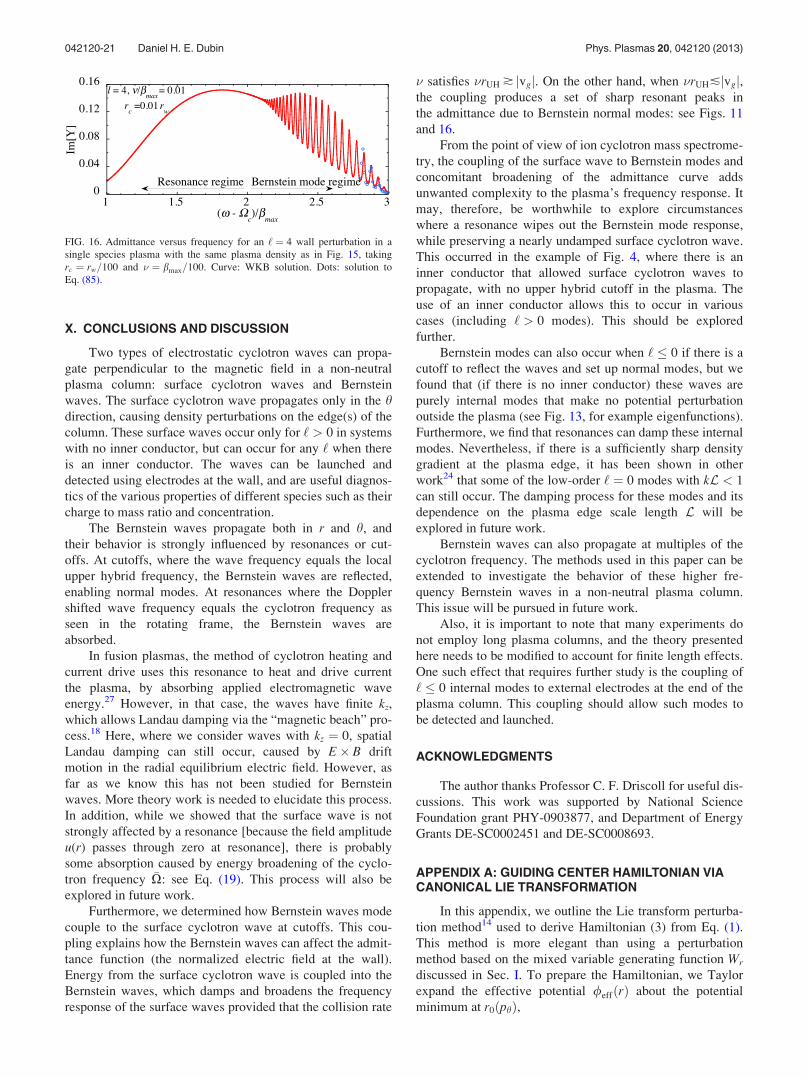
X. CONCLUSIONS AND DISCUSSION

Two types of electrostatic cyclotron waves can propa-

gate perpendicular to the magnetic field in a non-neutral

plasma column: surface cyclotron waves and Bernstein

waves. The surface cyclotron wave propagates only in the hdirection, causing density perturbations on the edge(s) of the

column. These surface waves occur only for ‘ > 0 in systems

with no inner conductor, but can occur for any ‘ when there

is an inner conductor. The waves can be launched and

detected using electrodes at the wall, and are useful diagnos-

tics of the various properties of different species such as their

charge to mass ratio and concentration.

The Bernstein waves propagate both in r and h, and

their behavior is strongly influenced by resonances or cut-

offs. At cutoffs, where the wave frequency equals the local

upper hybrid frequency, the Bernstein waves are reflected,

enabling normal modes. At resonances where the Doppler

shifted wave frequency equals the cyclotron frequency as

seen in the rotating frame, the Bernstein waves are

absorbed.

In fusion plasmas, the method of cyclotron heating and

current drive uses this resonance to heat and drive current

the plasma, by absorbing applied electromagnetic wave

energy.27 However, in that case, the waves have finite kz,

which allows Landau damping via the “magnetic beach” pro-

cess.18 Here, where we consider waves with kz ¼ 0, spatial

Landau damping can still occur, caused by E� B drift

motion in the radial equilibrium electric field. However, as

far as we know this has not been studied for Bernstein

waves. More theory work is needed to elucidate this process.

In addition, while we showed that the surface wave is not

strongly affected by a resonance [because the field amplitude

u(r) passes through zero at resonance], there is probably

some absorption caused by energy broadening of the cyclo-

tron frequency �X: see Eq. (19). This process will also be

explored in future work.

Furthermore, we determined how Bernstein waves mode

couple to the surface cyclotron wave at cutoffs. This cou-

pling explains how the Bernstein waves can affect the admit-

tance function (the normalized electric field at the wall).

Energy from the surface cyclotron wave is coupled into the

Bernstein waves, which damps and broadens the frequency

response of the surface waves provided that the collision rate

� satisfies �rUH � jvgj. On the other hand, when �rUH�jvgj,the coupling produces a set of sharp resonant peaks in

the admittance due to Bernstein normal modes: see Figs. 11

and 16.

From the point of view of ion cyclotron mass spectrome-

try, the coupling of the surface wave to Bernstein modes and

concomitant broadening of the admittance curve adds

unwanted complexity to the plasma’s frequency response. It

may, therefore, be worthwhile to explore circumstances

where a resonance wipes out the Bernstein mode response,

while preserving a nearly undamped surface cyclotron wave.

This occurred in the example of Fig. 4, where there is an

inner conductor that allowed surface cyclotron waves to

propagate, with no upper hybrid cutoff in the plasma. The

use of an inner conductor allows this to occur in various

cases (including ‘ > 0 modes). This should be explored

further.

Bernstein modes can also occur when ‘ � 0 if there is a

cutoff to reflect the waves and set up normal modes, but we

found that (if there is no inner conductor) these waves are

purely internal modes that make no potential perturbation

outside the plasma (see Fig. 13, for example eigenfunctions).

Furthermore, we find that resonances can damp these internal

modes. Nevertheless, if there is a sufficiently sharp density

gradient at the plasma edge, it has been shown in other

work24 that some of the low-order ‘ ¼ 0 modes with kL < 1

can still occur. The damping process for these modes and its

dependence on the plasma edge scale length L will be

explored in future work.

Bernstein waves can also propagate at multiples of the

cyclotron frequency. The methods used in this paper can be

extended to investigate the behavior of these higher fre-

quency Bernstein waves in a non-neutral plasma column.

This issue will be pursued in future work.

Also, it is important to note that many experiments do

not employ long plasma columns, and the theory presented

here needs to be modified to account for finite length effects.

One such effect that requires further study is the coupling of

‘ � 0 internal modes to external electrodes at the end of the

plasma column. This coupling should allow such modes to

be detected and launched.

ACKNOWLEDGMENTS

The author thanks Professor C. F. Driscoll for useful dis-

cussions. This work was supported by National Science

Foundation grant PHY-0903877, and Department of Energy

Grants DE-SC0002451 and DE-SC0008693.

APPENDIX A: GUIDING CENTER HAMILTONIAN VIACANONICAL LIE TRANSFORMATION

In this appendix, we outline the Lie transform perturba-

tion method14 used to derive Hamiltonian (3) from Eq. (1).

This method is more elegant than using a perturbation

method based on the mixed variable generating function Wr

discussed in Sec. I. To prepare the Hamiltonian, we Taylor

expand the effective potential /effðrÞ about the potential

minimum at r0ðphÞ,

FIG. 16. Admittance versus frequency for an ‘ ¼ 4 wall perturbation in a

single species plasma with the same plasma density as in Fig. 15, taking

rc ¼ rw=100 and � ¼ bmax=100. Curve: WKB solution. Dots: solution to

Eq. (85).

042120-21 Daniel H. E. Dubin Phys. Plasmas 20, 042120 (2013)

/effðrÞ ¼ /0ðrÞ þ1

2mr2ph þ

qB

2cr2

� �2

¼ /0ðr0Þ þe2

2mX2c

E2ðr0Þ þe4

m2r0X4c

E3ðr0Þ

þ 1

2mX2ðr0Þdr2 þ emX2

c

r0

dr3

� � 1

2þ 2e2Eðr0Þ

mX2cr0

� 1

6e2 E00ðr0Þ

mX2c

r0

!

þ e2mX2cdr4

r20

5

8� 5

2

e2Eðr0ÞmX2

cr0

� 1

24e2E000ðr0Þr2

0

!

� 3

4

e3mX2cdr5

r30

þ 7

8e4 mX2

cdr6

r40

þ Oðe5Þ ; (A1)

where dr ¼ r � r0ðphÞ, and where we have used Eq. (4). A

canonical transformation from r to dr is accomplished with a

type-2 mixed generating function,

F2ðr;PÞ ¼ ðr � r0ðPhÞÞPr þ hPh; (A2)

where capitalized momenta are the new momenta. This gen-

erator implies pr ¼ Pr; ph ¼ Ph, and it yields a new canoni-

cal angle coordinate H defined as

H ¼ @F2

@Ph¼ h� @r0

@phpr: (A3)

Next, we introduce lowest-order action-angle variables

ðw0; l0Þ [and corresponding new conjugate coordinates

ðH0; ph0Þ] using the usual definitions for the action-angle

variables of a harmonic oscillator,

dr ¼ffiffiffiffiffiffiffiffiffiffiffiffiffiffiffi

2l0

mXðr0Þ

scos w0; pr ¼ �

ffiffiffiffiffiffiffiffiffiffiffiffiffiffiffiffiffiffiffiffiffiffi2l0mXðr0Þ

psin w0: (A4)

The canonical transformation to these variables can be

accomplished using a second generator �F2ðdr;H; l0; ph0Þ

defined as

�F2 ¼ �dr

2

ffiffiffiffiffiffiffiffiffiffiffiffiffiffiffiffiffiffiffiffiffiffiffiffiffiffiffiffiffiffiffiffiffiffiffiffiffi2mXl0 � m2X2dr2

q

þ l0 cos�1 dr

ffiffiffiffiffiffiffimX2l0

s !þHph0

: (A5)

This generator implies that ph0¼ ph and that

H0 ¼@F2

@ph0

¼ H� @X=@ph

2Xl0 sin 2w0: (A6)

When written in these coordinates, the Hamiltonian has the

form

H?ðw0; l0; phÞ ¼ l0Xðr0Þ þ /0ðr0Þ þe2

2mX2c

E2ðr0Þ

þ e4

m2r0X2c

E3ðr0Þ þ eH1ðw0; l0; phÞ

þ e2H2ðw0; l0; phÞ þ ; (A7)

where

H1 ¼ �ffiffiffiffiffiffiffiffiffiffiffi2l3

0Xm

rcos3w0

r0

; (A8)

and H2, H3,… are not displayed due to their complexity.

The terms in H? involving w0 are transformed away

order-by-order using infinitesimal Lie transformations13,14

from coordinates z ¼ ðw0; l0;H0; phÞ to new conjugate coor-

dinates Z ¼ ðw; l; �h; �phÞ. The transformation is generated by

the following operator, defined by its action on a phase func-

tion f(z):

T f ¼XM

n¼0

ð�eÞn

n!wnf : (A9)

The operators wn are defined recursively in terms of their

action on f,

wnf ¼ ½wn�1f ; g ; w0 ¼ 1; (A10)

where ½ ; is the Poisson bracket for the phase space and g is

the generator of the transformation. Like T , g is also written

as a series in e,

g ¼XM

n¼1

en�1gnðzÞ: (A11)

A new Hamiltonian K(Z) is then obtained as a power series

in e via

K ¼ T H?: (A12)

The generators gn are chosen to remove the w-dependence

from the Hamiltonian, order-by-order in e. Writing K¼ K0 þ eK1 þ and expanding Eq. (A12) in e implies

K0 ¼ lX � H0;

K1 ¼ H1 � ½H0; g1;

K2 ¼ H2 � ½H0; g2 � ½H1; g1 þ1

2½½H0; g1; g1

�

(A13)

Also, coordinates are transformed according to

z ¼ T Z ¼ Z� e½Z; g1 þ Oðe2Þ: (A14)

Note that since Hn is independent of H0, so are gn and K.

Then, no derivatives of gn with respect to �h or �ph appear in

Eqs. (A13). Also, Eq. (A14) then implies that ph ¼ �ph.

At first order in e, Eq. (A13) implies that K1 ¼ 0 and

X@g1

@w¼ �H1ðw; l; phÞ; (A15)

which may be solved for g1 by integration. The constant of

integration is chosen so that g1 is periodic in w. Then, Eq.

(A14) implies that

042120-22 Daniel H. E. Dubin Phys. Plasmas 20, 042120 (2013)

l0 ¼ lþ e@g1

@wþ Oðe2Þ;

w0 ¼ w� e@g1

@lþ Oðe2Þ;

H0 ¼ �h � e@g1

@phþ Oðe2Þ:

(A16)

Working to Oðe4Þ, the result for the Hamiltonian is given in

Eq. (3). Also, application of the series expressions (A14)

[taken up to Oðe4Þ] to Eqs. (A6), (A4), and (A3) yields Eqs.

(13) and (14).

APPENDIX B: DERIVATION OF THEQUASI-EQUILIBRIUM DISTRIBUTION

In this Appendix, we outline the derivation of Eq. (24), the

expression for the quasi-equilibrium distribution function fqe.

One elegant approach employs a novel gyro-averaged collision

operator that keeps both short-range (Boltzmann) and long-

range28 collisions. This approach will be discussed in a separate

publication.29 Here, we employ a perturbation approach,

adapted from Ref. 16. The collision operator is assumed to be a

Boltzmann operator. Equation (22) is transformed from coordi-

nates ðr; vÞ to new coordinates ðr; v?;w0; vzÞ, where

vr ¼ v? cos w0; �vh ¼ v? sin w0; vr ¼ v r;�vh ¼ v h � evdðr; tÞ (B1)

and the drift velocity vd is defined by the solution of the

quadratic equation

v2d

rþ E

m� Xc

evd ¼ 0: (B2)

In these coordinates, Eq. (22) becomes

@f

@t� e

@vd

@tsin w0

@

@v?þ cos w0

v?

@

@w0

� �f þ v? cos w0

@f

@r

� erv? cos w0

@

@r

vd

r

� �sin b

@

@v?þ cos w0

v?

@

@w0

� �f

þ Xc

e� 2e

vd

r� v?

rsin w0

� �@f

@w0

¼ Cðf ; f Þ: (B3)

The solution for f is obtained as a power series in e and

� � �e=Xc, where � is the collision frequency [a frequency

scale factor on the order of C (f,f)/f]:

f ¼X1n ¼ 0

m ¼ 0

en�m fnm: (B4)

It was determined in Ref. 16 that @=@t is of order �e3, assum-

ing that @T=@r is of order e2 and @n=@r is O(1). For the

quasi-equilibrium, we therefore are concerned with terms of

order �0, i.e., fn0.

The lowest order equation is

Xc

e@f00

@w0

¼ 0; (B5)

which implies that f00 ¼ f00ðr; v?; vz; tÞ. The equation of

order e0�1 is

�@f01

@w0

¼ Cðf00; f00Þ: (B6)

Averaging both sides over w0 from 0 to 2p, and noting that

f01 is periodic in w0, implies that Cðf00; f00Þ ¼ 0, which

implies that f00 is a local Maxwellian,

f00 ¼ nðr; tÞ m

2pTðr; tÞ=m

� �3=2

e�mv2=2Tðr;tÞ: (B7)

Since Cðf00; f00Þ ¼ 0, Eq. (B6) then implies that

f01 ¼ f01ðr; v?; vz; tÞ. This function is determined at next

order in �

�@f02

@w0

¼ �Cðf00; f01Þ; (B8)

where �Cðf ; gÞ � Cðf ; gÞ þ Cðg; f Þ. A w0 average then

implies that �Cðf00; f01Þ ¼ 0. However, this implies that f01

¼ ðAðr; tÞ þ Bðr; tÞvz þ Cðr; tÞv2Þf00 (the collision operator

conserves particle number, parallel momentum, and kinetic

energy). When f01 is added to f00, this merely redefines

nðr; tÞ and T(r,t) (and allows a vz drift which we ignore), so

we can set f01 ¼ 0.

Next we consider f10, which must satisfy

Xc@f10

@w0

þ v? cos w0

1

n

@n

@rf00 ¼ 0 (B9)

[where we have used @T=@r ¼ Oðe2Þ]. The solution for f10 is

f10 ¼ h10ðr; v?; vz; tÞ �v?Xc

sin w0

1

n

@n

@rf00: (B10)

The function h10 is determined using the equation of order e1�1,

�@f11

@w0

¼ �Cðf00; h10Þ �1

Xcn

@n

@r�Cðf00; v?sin w0f00Þ: (B11)

In Ref. 16, it is shown that the second term on the rhs vanishes

due to conservation of momentum during collisions. Then, a

w0 average implies that �Cðf00; h10Þ ¼ 0, which implies, as

before, that we may set h10 ¼ 0, and we may set f11 ¼ 0.

In Ref. 16, working to higher order, similar arguments

were used to obtain f20,

f20 ¼ h20ðr; vz; v?; tÞ þKðr; tÞ4X2

c

v2?cos 2w0f00; (B12)

where

h20 ¼1

4X2c

1

n

@n

@r

� �2

v2? �

2T

m

� �f00 (B13)

and

Kðr; tÞ ¼ � 1

n

@2n

@r2þ 1

rn

@n

@rþ mXc

Tr@

@r

vd

r

� �: (B14)

Also, f21 was determined to be

042120-23 Daniel H. E. Dubin Phys. Plasmas 20, 042120 (2013)

�f21 ¼Mðr; tÞ

8X2c

�Cðf00; v2? sin 2w0f00Þ; (B15)

where

M ¼ �r@

@r

1

rn

@n

@r� mXc

T

vd

r

� �: (B16)

Finally, an expression for f30 was also obtained,

f30 ¼ h30ðr; vz; v?; tÞ �v?Xc

sin w0f00

mv2

2T2

@T

@rþ v2

?4X2

cn

@

@r

1

n

@n

@r

� �2" #

þ v2?

8X2cn

1

r2

@

@rr2nK � v2

?4Xc

m

Tr@

@r

vd

r

� � 1

n

@n

@r

( )

þ v?Xc

sin w0f00

3

2T

@T

@rþ T

2X2cmn

@

@r

1

n

@n

@r

� �2" #

� 2vd

Xcrn

@n

@r� r

Xcn

@

@r

vd

r

� � @n

@r

( )

� v3?

Xcnsin 3w0f00

1

24X2c

@

@r� 2

r

� �ðnKÞ þ rm

12XcT

@

@r

vd

r

� � @n

@r

" #: (B17)

However, the function h30 was not determined. Since we

require f30, we continue the derivation, using the Oðe3�1Þequation

�@f31

@w0

� v?Xcr

sin w0

@f21

@w0

þ v?cos w0

Xc

@f21

@r

� ¼ �Cðf00; f30Þ þ �Cðf10; f20Þ: (B18)

The function h30 is determined by integrating this equation

over w0. First, consider the terms involving f21. To evaluate

these, we note that the Boltzmann operator �Cðf ; gÞ has the

form

�Cðf ; gÞ ¼ð

d3vsdXsrðXs; uÞ u½f ðv0Þgðv0sÞ þ f ðv0sÞgðv0Þ

�f ðvÞgðvsÞ � f ðvsÞgðvÞ; (B19)

where rðXs; uÞ is the cross-section for scattering angle Xs,

u ¼ jv� vsj and the prime denotes post-collision velocities.

For f21, the collision integral involved in Eq. (B15) is

�Cðf00; v2?sin 2wf00Þ ¼

ðd3vsdXsrðXs; uÞ u f00ðvÞf00ðvsÞ

� ðv02?ssin 2w0s þ v02?sin 2w00� v2

?ssin 2ws � v2?sin 2w0Þ; (B20)

where ws is a variable of integration through vs, and w00 and

w0s are variables of integration through their dependence on

Xs. The operator has the following symmetry: if we define

new angles via ws ¼ w0 þ Dws;w00 ¼ w0 þ Dw0 and

w0s ¼ w0 þ Dw0s, the operator

ðd3vsdXs rðXs; uÞ u f00ðvÞf00ðvsÞ (B21)

is independent of w0, by the isotropy of the collision process

with respect to rotations about the z axis. This angle transfor-

mation transfers all w0 dependence to the four sin terms in

Eq. (B20), specifically sinð2w0 þ 2Dw0sÞ, sinð2w0 þ Dw0Þ,sinð2w0 þ DwsÞ, and sin 2w0. Therefore, f21 is a sum of two

terms, one proportional to sin 2w0 and the other proportional

to cos 2w0. This implies that

ð2p

0

dw0

2psin w0

@f21

@w0

¼ð2p

0

dw0

2pcos w0

@f21

@r¼ 0: (B22)

A similar argument implies that

ð2p

0

dw0

2p�Cðf10; f20Þ ¼ 0 (B23)

and that

ð2p

0

dw0

2p�Cðf00; f30Þ ¼ �Cðf00; h30Þ: (B24)

Thus, the w0 average of Eq. (B18) implies that�Cðf00; h30Þ ¼ 0, so we can set h30 ¼ 0. Therefore, to Oðe3Þ,the quasi-equilibrium distribution is

fqe ¼ f00 þ ef10 þ e2f20 þ e3f30 þ Oðe4Þ ¼ nðrÞð2pT=mÞ3=2

exp½�mDv2=2TðrÞ 1þe2rx0r0

4XcTmðv2

r � Dv2hÞþe3Dvh

(

� T0

2XcT3� mDv2

T

� ��

x0r0

4X2cT

m v2r þ

5

3Dv2

h

� �þ 2rT

n0

n

� ��

rx00r0

4X2cT

mðv2r þ

1

3Dv2

hÞ" #)

þ Oðe4Þ; (B25)

042120-24 Daniel H. E. Dubin Phys. Plasmas 20, 042120 (2013)

where Dv2 ¼ v2r þ v2

z þ Dv2h, Dvh ¼ v h � erxr0

, and xr0is

the rotation frequency for a thermal equilibrium system,

xr0ðrÞ ¼ 1

mXcrEðrÞ � TðrÞ

nðrÞ n0ðrÞ� �

þx2

r0ðrÞ

Xc: (B26)

When Eq. (B25) is multiplied by Dvh, integrated over v, and

divided by nr, one obtains a correction to this rotation fre-

quency due to shears, given in Eq. (28).

This expression for fqe can be converted into a function

solely of the constants of motion, Eq. (24), by substituting

Eqs. (9) and (13) for r, their time derivative for vr [using Eq.

(16)], and the time-derivative of Eqs. (11) and (14) for vh=r[using Eqs. (16) and (17)]. The result, in terms of r0, vz and

l, and independent of w, can be converted to Eq. (24) using

Eq. (4).

1A. G. Marshall and C. L. Hendrickson, Int. J. Mass Spectrometry 215, 59

(2002).2E. Sarid, F. Anderegg, and C. F. Driscoll, Phys. Plasmas 2, 2895 (1995).3R. W. Gould and M. A. LaPointe, Phys. Fluids B 4, 2038 (1992).4G. Pearson, Phys. Fluids 9, 2454 (1966).5R. W. Gould and M. A. LaPointe, Phys. Rev. Lett. 67, 3685 (1991).6R. W. Gould, Phys. Plasmas 2, 1404 (1995).7T. H. Stix and D. G. Swanson, “Propogation and mode conversion for

waves in nonuniform plasmas,” in Handbook of Plasma Physics, edited by

A. Galeev and R. Sudan (North-Holland, Amsterdam, 1983), Vol. 1.8P. L. Colestock and R. J. Kashuba, Nucl. Fusion 23, 763 (1983).

9A. K. Ram, A. Bers, S. Schultz, and V. Fuchs, Phys. Plasmas 3, 1976

(1996).10A. K. Ram and S. Schultz, Phys. Plasmas 7, 4084 (2000).11M. D. Tinkle and S. Barlow, J. Appl. Phys. 90, 1612 (2001).12R. S. Van Dyck, F. L. Moore, D. L. Farnham, and P. B. Schwinberg, Phys.

Rev. A 40, 6308 (1989).13H. Goldstein, Classical Mechanics, 2nd ed. (Addison Wesley, Reading,

Massachusetts, 1980).14R. G. Littlejohn, J. Math. Phys. 20, 2445 (1979).15L. S. Brown and G. Gabrielse, Rev. Mod. Phys. 58, 233 (1986).16T. M. O’Neil and C. F. Driscoll, Phys. Fluids 22, 266 (1979).17D. H. E. Dubin and T. M. O’Neil, Rev. Mod. Phys. 71, 87 (1999).18T. H. Stix, Waves in Plasmas (American Institute of Physics, New York,

1992).19D. E. Baldwin and D. W. Ignat, Phys. Fluids 12, 697 (1969); D. H. E.

Dubin, Phys. Plasmas 12, 042107 (2005).20P. Bellan, Fundamentals of Plasma Physics (Cambridge Univ. Press,

Cambridge, 2006).21I. S. Gradshteyn and I. M. Ryzhik, Tables of Integrals, Series and

Products (American Institute of Physics, New York, 1980).22R. C. Davidson, Physics of Non-neutral Plasmas (Addison-Wesley, New

York, 1998), Eq. (4.226). Note that xþ � x� ffi Xc � 2xE.23G. B. Whitham, Linear and Nonlinear Waves (John Wiley and Sons, New

York, 1974), p. 383.24G. W. Hart and R. L. Spencer, “Properties of axisymmetric Bernstein

modes in an infinite length non-neutral plasma” (to be published).25T. M. O’Neil, Phys. Fluids 24, 1447 (1981).26L. Rayleigh, Scientific Papers (Cambridge Univ. Press, Cambridge, 1899),

Vol. 1, p. 474.27N. J. Fisch, Rev. Mod. Phys. 59, 175 (1987).28D. H. E. Dubin, Phys. Plasmas 5, 1688 (1998).29D. H. E. Dubin, Phys. Plasmas (to be published).

042120-25 Daniel H. E. Dubin Phys. Plasmas 20, 042120 (2013)