Embed Size (px)
Citation preview

JADC 77157-30 NOR 76-190
WAVE DRAG REDUCTION FORAIRCRAFT FUSELAGE -WING CONFIGURATIONS
VOLUME 1: Analysis and Results
C .W. Chu, J. Der, Jr., H. Ziegler
Northrop Corporation Aircraft Division
FINAL REPORT OCTOBER 1977
Contract N62269-7S-C-0537 D D CAPPROVED FOR PUBLIC RELEASE; U1
DISTRIBUI-ION UNLIMITED
* INAVAL A IR DEVELOPMENT CENTERc::;~. Warminster, Pennsylvania 18974
c-,c

Best Available Copy
UNCIASS I F1 EDSECURITY CLAS•I't|CATION OF HlS PAGE f er1,r ) Data Entere.d)
774 PORT DOCUMENTATION PAGE ... ... ............ ...
I REPORT MJile.. - 2. GOVT ACCESSION NO. 3 kECIPIENT*S CATALOG NULIM8ER
NADC 77157-30
4. TITLE ('Mad Subt ft.) S ,TYPE OF REPORT II PFRIO0 COVEgiEo
WAVE DRAG REDUCTION FOR AIRCRAFT FinalFUSELAGE-WIN~G CONFIGURATIONS, 30 June 1975-30 Oct. 1976ý,
6.. PERFORMING 0, . RoPORT NUMEPVolume 1. Analyses and Results - NOR 76-1907 AuTHOR(SI a. CONTrACT OR GR1'r 4u rNsEtf,
N62269-75-C-0537C. W. Chu, J. Der, Jr., H. Ziegler
9. PERFORMING ORGANIZATION NAME ANO AODORSS 10 PROGRAM ELEMENT. PROJECT. TASKARCA A WORK UNIT NUMSERS
Northrop CorporationAircraft DivisionHawthorne, CA 90250
1 1 CONTROLLING OFFICE NAME AND ADDRESS 12- REPORT DATE
Naval Air Systems Command October 1976Washngtn, D C.13. wumeER OF PAGESWashington, D.C. .142
14. MONITORING AGENCY NAME &- A ORESS(d, j lIo.,0,,o C..troll-in Office) IS. SECURITY CLASS. (of trie t-110")
Naval Air Development Center UnclassifiedWarminster, Pennsylvania 18974 USc..DElassifice-N DOWNGRADING
SCHEOULE
16. 0ISTRIBUTION4 STATEMENT (of thisi Report)
Approval for Public Release, Distribution Unlimited
17 oIST-rISUTION STATEMENT (.1 he .6.(bt•a, r ".fIrd in Block 20, It dillf nr from e'palt)
18. "UPPILEMENTARY NOTES
ill. KCEY WORDS (Continue Oft reverse side it nocessary swIi Identify by block Iii~iil.r)
Wave Drag, Three-Dimensional Flow, Supersonic Flow, Characteristics Methods,Aircraft Fuselage, Wing-Body Configuration, Optimization, Latin Squares,Numerical Method
20. A13STIRACT (Co.~elnuo os rverse. uid& if riseposaW and identify by block numb..)An optimization procedure has been developed to minimize the wave drag of an
aircraft fuselage-wing configuration subject to constraints imposed by design require-ments. The theory, methods, computer programs and results are presented in thisreport in two volumes. Volume {idescribes analyses, results and the optimizationprocedure. The procedure makes ruse of the Latin Square sampling technique and theThree-Dimensional Method of Characteristics. The former is used to efficientlysample the family of configurations, and the latter Is uscd to accurately calculate the
DDI A7, 1473 LoTIoN O, a NOV 65 IOSOLT. UNCLASSIFIEDSgCURITy Cl.ASSI"II•ATION Oft THIS PACE ( D• #fta Enlered)

Best Available CopyUNCLASSIFIED
SEC URirY CLASSIIICATION OF THIS PAGE(WWhani Daeta Enerad)
20.
wave drags of the sampled configurations. The calculated wave drag coefficients arethen used to derive a functional dependence of the wave drag on the geometric variablesthat define the family of configurations. The minimum wave drag configuration car, beobtained by minimizing the wave drag function subject to a given set of constraints.The wave drag reduction procedure is demonstrated using an F-4 type configurationas the baseline. The results are presented and discussed.
Volume II is the user's manual for the computer programs. The input/outputinformation is described in detail. Listings of the programs are given, and samplesof built-in program diagnostic messages are explained. Also included are the logicalstructures of the programs and the descriptions of the subroutines, which in combina-tion with the program listings can be used for possible future modification, improve-nient, or extension of these computer programs.
UNCLASSIFIEDSECURITY CLASSIFICATION OF TW#S PAGJAOWh0M D.aa K.t,..dE

Best Available Copy
FOREWORD
This wo; k was ptrformed I)y the Aerodynamics Research Organization of
the Aircra't Division of the Northrop Corporation in Hawthorne, California for
the Y.a:al Air Deveiopment Center in Warminster, Pennsylvania (Contract No.
"N62269-75-C-0537) under the auspices of the Naval Air Systems Command. The
contract monitor wc.s Mr. Carmen Mazza of NADC, whose cooperation and
assistance are gratefully acknowledged. The authors are indebted to Messrs.
William Becker, David Bailey ajnd K. T. Yen of NADC for their valuable assis-
tance during the course of this work. Special thanks go to Messrs. Ray Siewert
and Louis Schmidt of NASC for their encouragement and interest in the present
work.
"fill I Wt b l (NO
ODCJUN 28 M
~ ~~~~~E F17'...- Ii II f
iii

Best Available Copy
TABLE OF CON1TENTS
Section Page
1. INTRODUCTION ......... ............................ . .
2. FORMULATION AND METHODS .............................. . 4
a. Formulation.............................................4
b. Latin Square Sampling Technique ........ ............... . 5
c. Three-Dimensional Method of Characteristics ................. ... 6
3. DESCRIPTION AND VARIATION OF FUSELAGE-WING
CONFIGURATION ............. ............................ 7
a. Body Description ........ ............................... 7
b. Fuselage and Canopy ................................... 8
c. Wing and Blending ........ .............................. 10
d. Geometric Variables and Variations .......................... 13
4. FLOW FIELD CALCULATION AND WAVE DRAG REDUCTION .......... 16
a. Calculation of Flow Fields . ................................ 16
b. Wave Drag Equation ........ ............................ 18
c. Variation of Wave Drag with Geometric Variables ................ 19
d. Optimizaion and Minimum Wave Drag Body ...................... 21
e. Summary of Wave Drag Reduction Procedure ................... 23
5. CONC LUSIONS ............................................. 25
REFERENCES . ............................................. 27
APPENDIX A - WAVE DRAG REDUCTION FOR FORWARD"FUSELAGES.. ......................... Al
APPENDIX B - THE LATIN SQUARE METHOD ..................... B1
APPENDIX C - BODY DESCRIPTION METHOD.. ..... ..... . .
APPENDIX D - NUMERICAL SEARCH FOR MINIMUM PROCEDURE .... D1
APPENDIX E - DEMONSTRATTO? OF LATIN SQUARE PROCDURE.... Z
V -r Zi - 1J
pr zW~fO ?AGEL~C.OT1

Best Available Copy
I L LUKST ,TIONS
Figure pg
1. Schematic of Fuselage and Wing Cross Sections Description ........... 30
2. Geometric Variables for Fuselage Variatiori and Wing-RodyBlending ............. ................................... 31
3. Sample Distributions of Miending Radius r ...... .................. 32
4. Pressure Distributions Along Centerlines and Wing LeadingEdge of F-4 Type Baseline ....... ....... ................... 333
5. Cross Section of F-4 Type Baseline at Fuselage Station 430 ............ 34
6. Front Views of F-4 Type Baseline Cross Sections ................... 35
7. Front Views of Configuration 6 Cross Sections ..................... 36
8. Cross Section and Pressure Distribution at F. S. 350 of BlendedWing Configuration 6 .......... ............................ 37
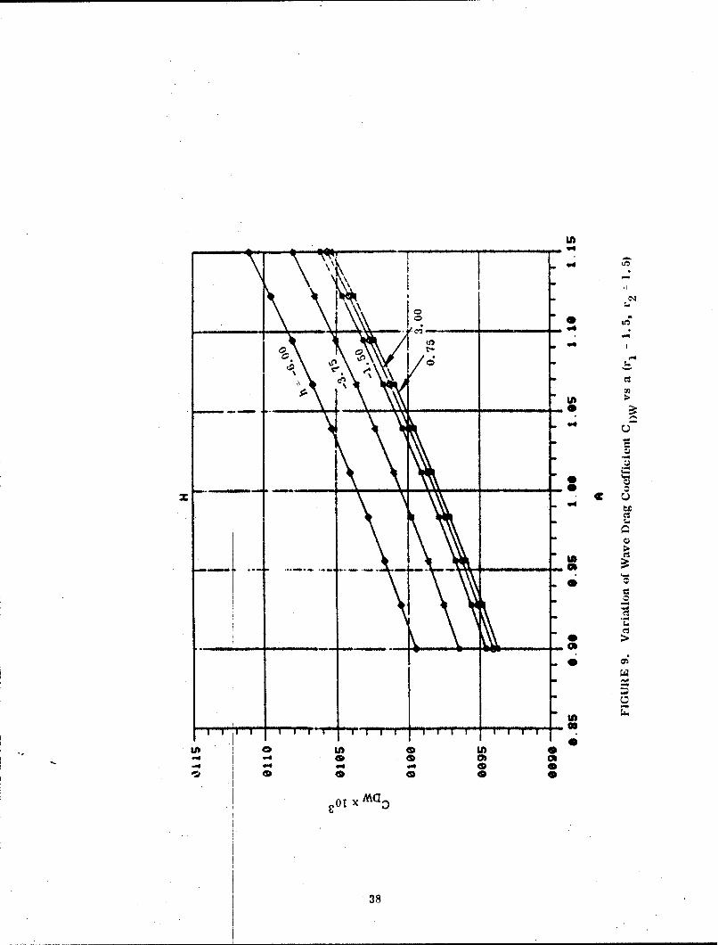
9. Variation of Wave Drag Coefficient CDW vs a (r1 *1. 5, r 2 = 1.5) ..... .38
10. Variation of Wnve Drag Coefficient CDW vs a (r 2 = 1.5, h -0 .......... 39
11. Variation of Wave Drag Coefficient CDW vs a (r1 =1.5, h= 0) ........ 40
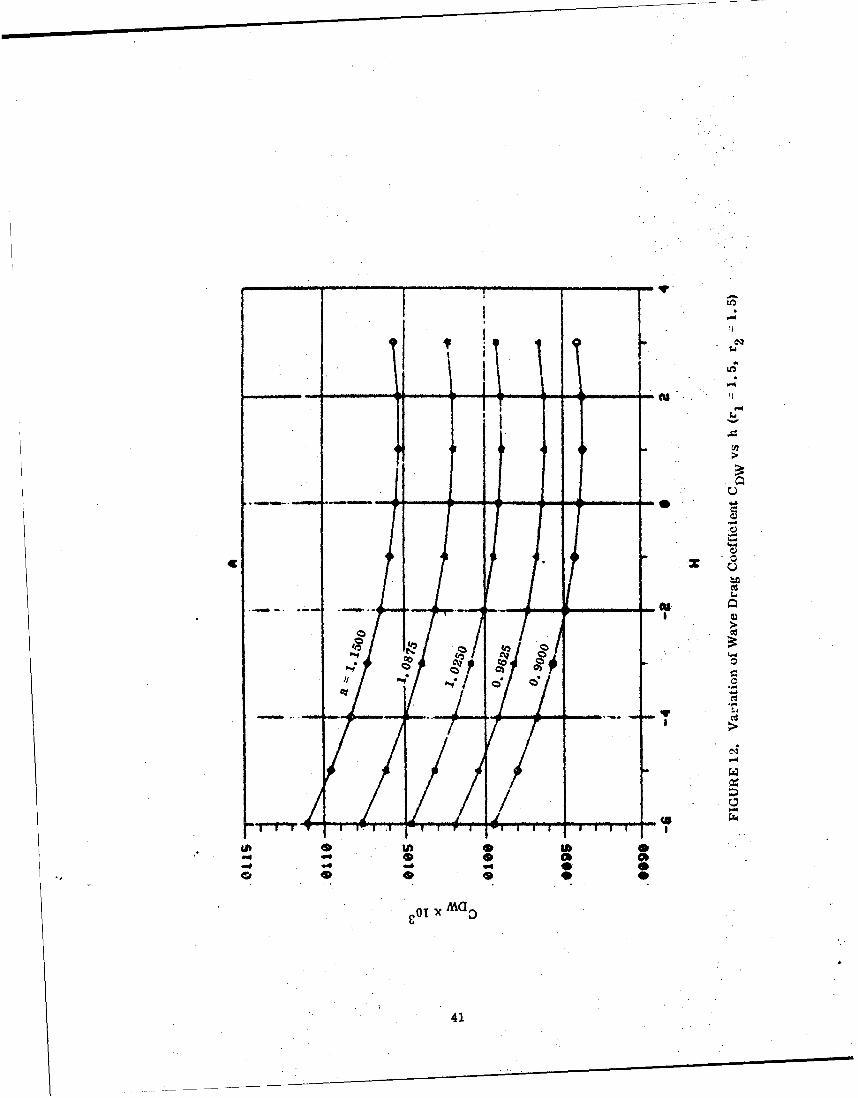
12. Variation of Wave Drag Coefficient CDW vs h (r1 = 1. 5, r 2 1.5) . . . .. 41
13. Variation of Wave Drag Coefficient CDDW vs h ( a 1.0, r 2 11.5) ...... .42
14. Variation of Wave Drag Coefficient CDW vs h (a 1.0, r= 1.5) ...... .43
115. Variation of Wave Drag Coefficient CDW vs r1 (r 2 = i. 5, h = 0) ........ 44
16. Variation of Wave Drag Coefficient CDW vs r1 fa 1.0, r2 = 1.5) ..... .45
17. Variation of Wave Drag Coefficient CDW vs r1 (a = 1.0, h = 0) ......... 46
18. Variation of Wave Drag Coefficient CDW vs r2 (r! = 1.5, h = 0) ........ 47
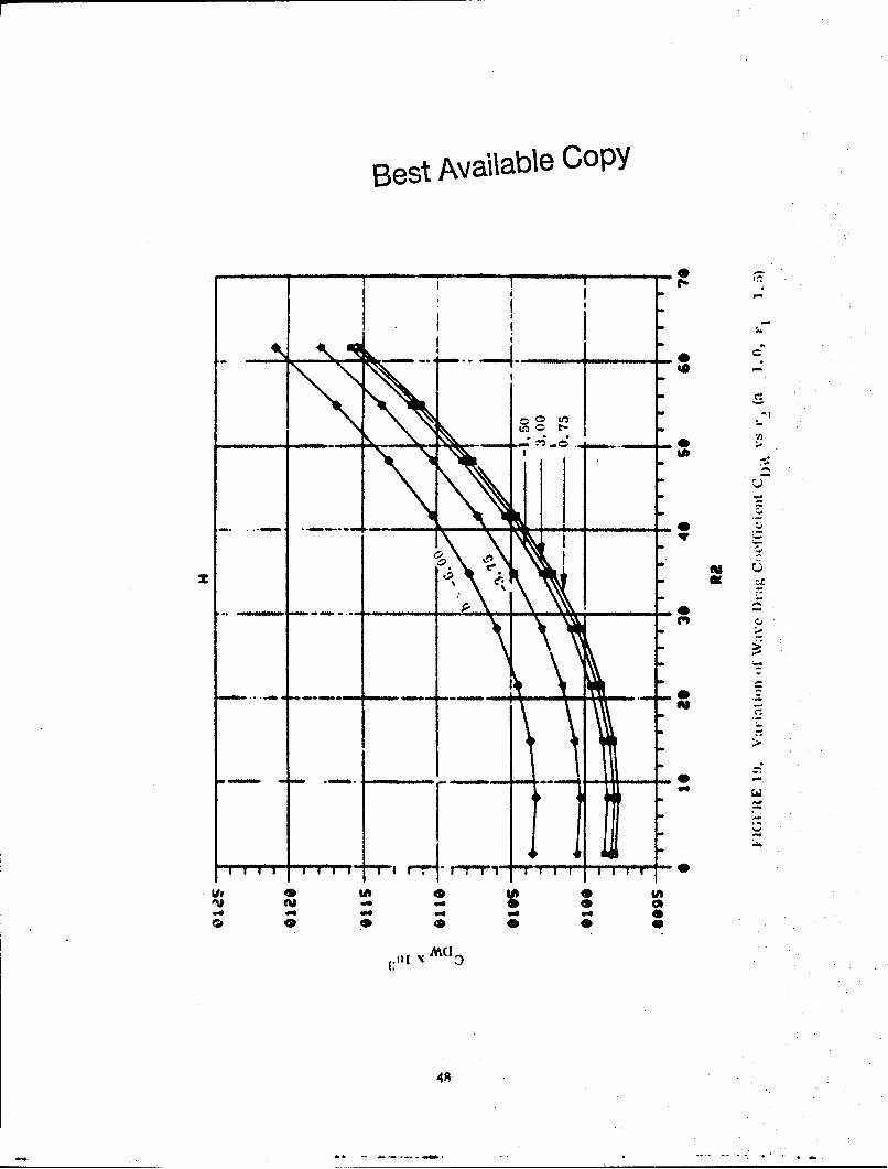
19. Variation of Wave Drag Coefficient CDW vs r 2 (a = 1.0, r== 1.5) ...... .48
20. Variation of Wave Drag Coefficient CDW vs r 2 (a =1.0, h 0) ........ 49
21. Front View of a Minimunt Wave Drag Body ..... ................. 50
22. Minimum Wave Drag Configurations for Various Volumes({ of Baseline Volume) ........ ............................ S1
vi

Best Available CopyTABLES
Table Pag
1. Latin Square Arrangement .................................. 28
2. Variables, Ranges, and Baseline Values ......................... 28
3. Wave Drag Coefficients CDW ......................... 29
4. Coefficients of Wave Drag Equation .. . . ....................... 29
vi.

Best Available Copy
IIST OF SYM BOLS
a Horizontal displacement of the maximum breadth line
a , aij Coefficients of wave drag Equation (1)
bo, bi, bij Coefficients of wave drag Equation (28)
b Shape factor for the lower fuselage cross section
C DW Wave drag coefficient
C P ressure CoefficientP
f Width of the fuselage bottom flat
h Height of the lower deck
I Length of the fuselage nose
P., Qj, R., S., T. Coefficients for the jth generating line
r 1 , r) Blending radius
Vol Volume of the fuselage
VolBL Volume of the baseline fuselage
X, Y, Z Rectangular coordinates
x i ith geometric variable
X.(Y) Projection of the jth line on the X-Y plane
z i ith reduced variable
Z (Y) Projection of the jth line on the Y-Z plane
viii
Best Available Copy
1. INTRODIICTION
Wave drag reduction is one of the important goals of designing a high perfor-
mance aircraft capable of operating in the supersonic regime. Since there are many
design requirements which conflict with one another as far as wave drag reduction is
concerned, an optimization procedure is needed to determine the minimum wave
drag configuration subject to the constraints imposed by these requirements. Until
recently, the procedure relied heavily on experience gained through extensive wind
tunnel testing of various geometries. Such a design procedure, which usually could
not be carried out systematically, was cKpensive and time consuming. However,
the advancec ýf recent years in numerical methods and computer technology have
made feasible systematic optimization procedures using exact numerical methods,
Consequently, a wave drag reduction procedure using the method of characteristics
has been developed which is presented in this report.
The present wave drag reduction procedure makes use of two basic methods:
the Latin Square sampling technique and the Three-Dimensional Method of Character-
istics. The former is used to select sample configurations so efficiently that a
small number of samples -tan well represent the entire family of configurations.
The latter is used to calculate accurately the wave drags of the sampled configura-
tions. Briefly stated, the present approach consists of calculating the wave drag
of a baseline configuration and some variations specified by the Latin Square sampl-
ing technique, determining a functional dependence of the wave drag un these varia-
tion parameters, and minimizing this wave drag function to obtain the configuration
with minimum wave drag. The procedure is general with respect to the number of
geometric parameters (or variables); the higher the number, the larger the required
Latin-Square size. The computer programs developed under this study cover the
most often used 3 x 3 and 5 x 5 Latin Squares.

Best Available Copy
The complete wave drag reduction program has been. carried out in two phases.
In the first phase, a procedure was developed for minimizing the wave drag of a
forwaCd fuselage and eanol)y config•,ration as rcported in Reference 1. In the
stvotid phase, the procedure has been expanded to account for the influence of the
wing and wing-body blending on the overall wave drag. In this final report, the
research performed under the wave drag reduction contract is presented. The
phase I work, which was reported in Reference 1, is Included as Appendix A for
ready reference, whereaa the main text of the report presents the phase 11 work
and tou'.hes upon some of the phase I work. A 3 x :3 Latin Square was used in phase
II and a 5 x 5 Latin Square in phase I. The surface fitting method using Latin
Squares as presented in Reference 2 was improved during the phase I study; the
improvement which is presented in Appendix A, is essential for the success of the
optimization procedure (here applied to wave drag reduction). The procedure using
the improved Latin Square surface fitting method has been proven in both phases
through application to the F-4 configuration. For further .validation of the procedure,
it was applied to the von Karman ogive. For given configuration length and base,
the present optimization procedure correctly predicted the von Karman ogive as
the minimum wave drag body.
In this report, the basic approach is given first, which consists of the formu-
lation of the problem and a brief account (f the two basic methods, It is followed by
a discussion of the method of describing the body and the selection of'geometric
variables and their ranges for defining a family of configurations. Then the flow
field calculation and the wave drag equation are presented. Sample results of the
calculated flow fields are given, and calculated wave drag coefficients are tabulated.
These coefficients were used to derive the wave drag equation which expresses the
wave drag as a function of the geometric variables. Once the wave drag equatien is
obtained, the dependence of the wave drag on the geometric variables is established.
2

Best Available Copy
A set of figures are given to illustrate some of the characteristics of the wave drag
",quation. This is followed by a prcsentation of the optimization procedure and the
prediction of the minimum wave drag body. Finally, conclusions are drawn and some
recommendations given. The Latin Square technique including the method of con-
struction is presented in Appendix B. A discussion of the general body description
method is given in Appendix C. The Numerical Search Procedure for the minimum
wave drag configuration is presented in Appendix D. The validation of the optimiza-
tion procedure using the von Karr'an ogive is presented in Appendix E.
3

Best Available Copy
2. I ()lIR.V IATI()N AND) M\EI('ll)I
"Tlhe' wave drag. (t) a cofi• inui"rat ion is a functif, it , a number of factors. Fo I.
given ftli,rht conditions the wave dra- dtlpends (in how the cnfiguration is shaped.
"Since the shape i)f ;in airc rait, at l east in the initial desig-n phase, is mainly
determined bVy COnsider.;tti(ons other than the wave .rag, it is practical to c,,nsider
the probl)lem otf reduing the wave drag o(o a given baseline cnhiYr'ti)n )y
tbtaining a variation configuration thai satisfies all the desigii c,,nst raints yet has
the least wave drag. Such a baseline configuration could be a new configuration
at a certain stage of devel opne,,ent or it could be an existing airplane that is to be
m•dxified or improved.
In this section, the formulation of the wave drag roduction problem is outlined,
and the two basic methods to be used in this study are introduced.
a. Formulation
The baseline configuration can be described by a set of geometric variables.
A family of configurations including the baseline caxn be generated by assigning
different values to some or a:! of the geometric variables. If the wave drag can be
expressed as a function of these variables, a particular set of values of these
variables that gives the least wave drag can be found by minimizing the function.
This set of values then produces the minimum wave drag configuration.
The key to this problem is how to obtain such at functional axpression for the
wave drag. For the present study, four geometric variables are considered in
defining the family of configurations. If each varibj)le assumes three values, the
evaluation of the partial derivatives with. respect to these four variables for a Taylor-
series type expression would require 81 wave drag calculations. It will be shown
that through Latin Square sampling the present procedure proves useful using only
4.

Best Available Copy
10 wave drag calculations. In the present approach, the wave drag coefficient CDW
is first assumed to be of the form
4C - aItxi 4 t.x x
CDW 0a i ( 1\ x ) a (1)
where x.(i 1, 4) are the geometric variables and a. and a.. are to be determined.9
The Latin Square sampling technique is used to samnple 9 sets of values of x.
out of the total population of 81 sets. The wave drag coefficients for the F-4 type
baseline and the configurations defined by each of the 9 sets are then calculated
by the Three-Dimensional Method of Characteristics. 3,4 When the 10 calculated
wave drag coefficients CDW and the corresponding ,alues of the geometric
variables "i are substituted into Equation 1, 1 ) linear equations for the 10 un-
knowns ai and aij are obtained. These equations are then solved for the ai and
aij, which are substituted back into Equation 1 to produce the functional expres-
sion for the wave drag in terms of the geometric variables. By minimizing
CDW in Equation 1 subject to a given set of cr ,straints, e. g., a given volume
of the aircraft, the minimum wave drag configuration corresponding to the given
set of constraints is 'etermined. In the present study, a numerical search pro-
cedure is used to lind the mlnim,,_m wave drag configuration (Appendix D).
b. Latin Square Sampling Technique
The Latin Square method, which has mostly been used in agriculture and
biological resear,.:h, is a very efficient sampling technique and is much better than
4 random sampling. For this study a particular type of Latin Square (the orthogonal
squares) suitable for a variety of technical problems2 is adopted. With this type
of Latin Square arrangement, a 3 x 3 square is the correct size for four geometric
variables xi, each taking three values. It is convenient to introduce the reduced

variables zi, which are related to the geometric variable xi through
X x. z. (xi -x )max min max minl 2 2()
where subscripts max and min denct2 the maximum and minimum values,
respectively. Corresponding to the three values of the geometric variables xi,
the reduced variables z. alwvys asume the three levels of 0, ! 1. The 3x3i
Latin Square arrangement in terms of the levels of the reduced variables and
the cell number is shown in Table 1. * It is seen that in this way, the Latin
Square arrangement remains the same whatever the values of the geometric
variab, es.
c. Three-Dimensional Method of Characteristics
In this study the Three-Dimensional Method of Characteristics 3' 4 is used to
calc.date the wave drag coefficients for the fuselage-wing configurations sampled
by the Latin Square technique. This method has been previously applied to cal-
culate the flow fields over a Aide varty.y of configurations including spherically-
capped three-dimensional bodies and wings 5 , aircraft fuselages and wings at
general angles of attack,6 and slab delta wings and space shuttle wing-body con-
figurations. - Whenever experimental data were available for comparison, good
agreement between theory and experiments was observed. The capability of
treating the canopy, however, was developed during phase I of this study.
Tn a related research program, theThree-Dimensional Method of Characteristics
was further extended and improved to treat realistic aircraft wing-body configura-
tions including wing-body blending. With some modifikation and adaptation, this
Improved method was applied to calculate the flow fields and wave drags of the
variation configurations.
*A discussion of the Latin Square construction is given in Appendix B.

3. DESCRIPTION AND VARIATION OF FUSELAGE-WING CONFIGURATION
Three-dimensional body description requires a great deal of effort which at
times becomes extremely tedious. Basically, two types of description can be
made, analytical and numerical. The latter can describe complicated geometry
accurately, but is cumbersome for preparing input data. The former is much sim-
pier to input and can define a family of configurations based on a few geometric
variables. Hence, analytical description is chosen for the present study.
a. B T)escription
Every configuration has P. number of generating lines, such as the upper
profile, the lower profile, the maximum breadth line, or the wing leading edge.
In the present body description procedure, each generating line is divided into a
number of segments to permit each segment to be described by a conic-section
curve. At each c ross section of the configuration, simple analytic curves, e. g.,
the ellipse or cubic, connect any two adjacent generating lines to form the contour
of the cross section. The configuration is thus described analytically by simple
low-order curves. For a smooth body a unique normal to the surface exists every-
where, and this condition usually requires slope continuity at the junctures between
two contour curves or two segements of a generating line.
The fuselage is located in a right-handed coordinate system where the Y-axis
is aligned with the fuselage axis; the X-axis is spanwise and the Z-axis is up. All
generating lines are represented by a general curve fit of conic sections in several
segments. The coric-section curve takes the form
(Z P Q Y RY2 SY+T 1/2
A straight lhie is a special case with R S T 0. Each curve can
7

be divided into as many se, ,ments as necessary to provide adequate body description.
Each segment must be continuous with the previous segment and with very few
exceptions the slope must be continuous at the junctures to satisfy the requirement
of a unique normal to the surface.
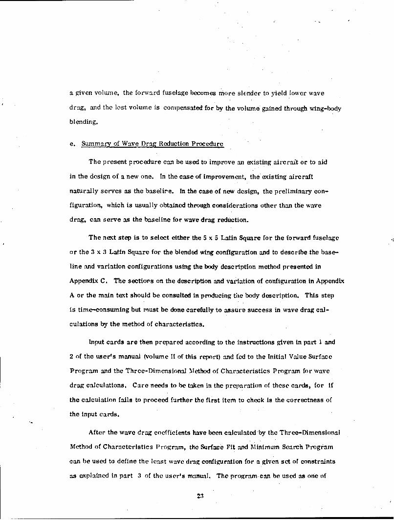
A typcial cross section of thewing-body configuration is shown schematically
in Figure 1. The contour of the cross section begins with a straight line represent-
ing the canopy flat. The canopy contour from points C to 0 is circular but can be
elliptic in general. The upper fuselage is represented by an elliptic curve from
points U. to M. A straight side flat from points M to Ff joins the upper fuselage
to the lower fuselage, which is also represented by an elliptic curve from Ff to L.
A straight line from point L to the centerline describes the bottom flat. For the
description of the wing, straight lines E G and F H represent the upper and lower
surfaces of the wing, respectively. Partial eliipses G I and H I complete the wing
description near the leading edge L. The wing-body blending is effected by circular
arcs 34 and 56 with radii rU and rL, respectively. A further discussion of the
body description method illustrated by the description of the fuselage and canopy
of Phase I is presented in Appendix B.
b. Fuselage and Canopy
The equation of the canopy is given by
-- 1 0 (4)
If it is a circular arc, then (ZO- Zc) 2 (Xc X,) 2 . The equation for the upper
fuselage is
z 12 [ Y X (Y)
z Y Y X M(Y) X U(Y) - = 5
8

The intersection between the canopy and fuselage is faired by a cubic from
points 1 to 2 (Figure 1). The projections Z1Y) and Z2 (Y) of lines 1 and 2 on the
Y-Z plane are given by Equation 3 where the coefficients P, Q, R, S, T are input
quantities. The projections X1 (Y) and X2 (Y) on the X-Y plane are obtained by
solving Equations 4 and 5, respectively.
xi(Y)-xc+(X0 xc) i(- z 0)2 I1/ (6)
x2 (Y) xt + (XI, - xu) - )2 1 (7)
The fairing curve matches the slopes of the ellipses at both end points 1 and 2. The
slopes are obtained by differentiation of Equation 4 and 5
(IX z- I - z G,)(x 0 ) 2 (8)
1 2(Y) ( =X (-2 ZZ)(XX o
M M 12x (z2 XU' Zu 2 M
The cubic equation that satisfies Equations 6 and 8 can be written
2 x - zI z z .3
The coefficients c and d are obtained by applying Equations 7 and 9
c a 3(X 2 -x 1)-(X2 + (z2 -zX) (11)d =-2(X 2 -X ) + (XV + XI) (Z -Z ) (12)
Equation 10 with c and d given by Equations 11 and 12 is then the cubic equation for
9

the fairing curvo from points 1 to 2. The quantities X1 , X2 , XI and X' are given
by Equations 6 and 7 while XU, XM, XC, X0, ZUT ZM, ZC 0 t zip andZ2
are obtained from Equation 3 where coefficients P, Q, R, S and T are input
quantities.
The lower fuselage is described by an equation similar to Equation 5
2 2
[1;$ f + x]2 [ X..L (Y) - (13)
Z E Zf(Y (X - XL(Y) 2
All flats are given by simple straight-line equations.
c. Wing and Blending
The upper and lower surfaces of the wing are given by straight-line equations
for E G and F H. Near the leading edge I, the partial ellipses G I and H I are
derived as follows. The equation may be written in the form
(x- +a)2 (Z -ZI) 2I + - =Z 1 1 (14)
a2 b2
where a and b are the axes to be determined. Differentiation of Equation 14 gives
X = XI + a Z - ZI dZ (= ..... + - - = 0(I
a 2 b2 dX
at point G, X XG, Z= Z., and- = A , which is the slope of line E G.. Sub-
stituting these values into Equation 14 and 15 leads to
2 (zr - zT) 2-:G1- .. + (14a)
a2 b2
XG XIa XGZ (dZ) 0 (a)
b2 2 0X
10

Elimination of b2 froar Equations 14a and 14b yields
2 dZI
C (dXI) G - "9 I(ZG ZI)adZ = (16)
ZG -zI -2XMI) d=Z
Elimination of a2 from Equations 14a and 14b leads to
( ) Z (X-X, +a) dZ (17)G2 - ZI)2_Z - "I)(X )G
where a is given by Equation 16. Equation 14 with a and b given by Equations 16 and 17
describes the partial ellipse G I. By changing the subscript G to H, the equation for
the partial ellipse H I is obtained.
The projections of lines passing through E, F, G, H and I on the Z-Y plane
and X-Y plane are input quantities for defining the wing. In order for the partial ellipses
to exist, points G and H must be located within a certain range, which depends on the
relative positions of these five points. When the wing span is very small, It is difficult
to input both projections of lines through G and H such that these points are located within
acceptable ranges. In such cases, the X coordinates of G and H are calculated inside
the program to satisfy the range requirement.
The upper and lower blendings between the fuselage and the wing are described
by circular arcs with radii r U and rL, respectively. When the blending radii rU and
rL are specified by geometric variables (see Section 3d.), points 3 and 5 of Figure 1
can be obtained numerically through an iteration procedure. However, in order to
oitain analytical normals to the blending surface, an analytic expression must be derived.
Hence, the following procedure was used and is illustrated by the upper blending. The
numerically obtained line paessing through point 3 is considered a generating line. The
projection Z3 (1) on the Y - Z plane is expressed in the form of Equation 3, where
11

the coefficients are input quantities. At a given fusalage station, X3 (Y) are obtained
by solving Equation 5.
/2j1/2
x 3y = (xM-xU)I I 21 UZ(18)
The slope of the tangent at point 3 can also be obtained from Equation 5 as
M3 U - ) 2 x 3~-z (19)
Thus, the equation of the tanigent 3 (see Figure 1) at point 3 is given by
Z =C M 3 (X-X 3 ) 3 Z3 (20)
The equation of line E G can be written as
Z = M4 (X -XE) - ZE (21)
where M4 XG _ XE (22)
Intersection P of these two lines is obtained from Equations 20 and 21
Z -z * MX -4M XXp 3 M3 M3 4 E
M 4M3 4!(23)
) M3 Z M4Z3 4 M3 M 4 (X 3 -X5Z Mt -M 43 3
p N ... . 3 M4
The equation of the line bisecting the angle Z 3PG is given b'
Z M 5 (X-XPX) + Zp i (24)
taj -1 ÷ i-
where M tan r+tan M +tan ) 4aw M5 2(24a)
12

and M3 is given by Equation 19 and M4 by Equation 22. The intersection between
the bisecting line and the normal at point 3
X-X 3 . M3 (Z- Z3 ) 3 0 (25)
is the center 0 of the arc; hence from Equations 24 and 25
X ±MZ +M.(MX - Z)X0 = 3 M3M5
(26)
Z, - M5 Xp + M5(X 3 - M3 Z3 )
o1 '- M M
where Xp and Zp are given by Equation 23, M3 by Equation 19 and M by Equation
24a. The equation of the circular arc for the upper blending is thus
(X _ Xo)2 + (Z - Zo2 2 2 2 R2 (27)(- 0) +( 0 ) =(XO -X3) + (ZO - Z3) RU (
where X0 and Z0 are given by Equation 26. Notice that the radius RU is slightly
different from rU because of slight errors introduced by the ite.ration procedure
in obtaining point 3 and by the fitting of the generating line passing through that point.
d. Geometric Variables and Variations
Four geometric variables were selected to generate a family of fuselage-wing
configurations including the F-4 baseline. As illustrated in Figure 2, these
variables are the horizontal displacement a of the maximum horizontal breadth
line, the lower deck height h (which increases as the lower profile is raised),
and the blending radii r1I and r 2 at F. S. 280 and F. S. 360, respectively. All
configurations generated by these variables have the same canopy as the F-4 and
must satisfy the over-the-side view line limitation. The correspondence between
13

the geometric variables and the reduced variables defined in Equation 2, the
ranges of variation ot these geomeiric variables, and the baseline values of these
variables are tabulated in Table 2.
The geometric variables specify the blending radii at two fuselage stations
only. In order to fully describe the blending between the fuselage and wing, a pro-
cedure is needed to provide the blending radius systematically at any given fuselage
station in the blending region. The blending radius distribution as a function of the
fuselage station must satisfy the following conditions:
1. At fuselage stations 220 or 430, the radius is equal to the minimum radius of
the baseline.
2. At F. S. 280 and F. S. ,60, they are equal to r 1 and r 2 , respectively.
3. Between F. S. 280 and F. S. 360, the radius must not overshoot; i. e., it must
not exceed the greater of r 1 and r 2 .
4. When r 1 and r 2 are equal to the minimum radius, the baseline must be
recovered; i.e., the radius must be constant throughout.
5. When either r 1 or r 2 is equal to the mrinimurn radius, the blending radius must
not undershoot anywhere.
Figure 3 illustrates some of the possible radius distributions and serves as a
reference for the foliowing discussion of the procedure. The radius distribution is
given by three cubic interpolation formulas for the three intervals. The slope of the
distribution curve is zero at F. S. 220, 280 and 360 for r = 1.5 and at F. S. 280 and
360 for r = 61.5. At F. S. 280 the slope at r = 46.5 is assumed to be equal to that
of the straight line S . At any other r the slope is obtained from a spline fit of the
slope versus r in such a way that the spline curve passing through these three points
with assumed zero curvature at both end points. The slopes at F. S. 360 are obtained
in an anologous way. Thus, for a given pair of r1 and r2, the radius distribution curve
is determined by three cubic interpolation formulas: the first cubic passes through
14
r 1.5 at F. S. 220 with a zero slope and r r at F.S. 280 with a slope given
by the spline fit: the second cubic passes through r r at F. S. 280 with the same
slope as the first cubic and through r = r 2 at F. S. 36;0 with a slope given by the
second spline fit; the third cubic passes through r = r at F. S. 360 with the same
slope as the second cubic and through r = 1. 5 at F.S. 430 with an assumed zero
curvature. The radius distribution curve as composed of these cubics are then
described by conic-section curves for input into the computer programs.
While the lower blending radius could be varied, its range would be very
much limited in the case of the F-4. Therefore, a fixed lower blending is
used to assure a smooth body for the 3DMoC calculations. This blending is
specified by assigning a fixed distance between points 5 and F (see Figure 1).
15

4. FLOW FIELD CALCULATION AND WAVE DRAG REDUCTION
Once the geometric variables and their ranges of variation have been selected,
the fuselage-wing con figuration, corresponding to the nine cells of the 3 x 3 Latin
Square can be described. The Three-Dimensional Method of Characteristics to-
gether with a blunt body program for providing the initial data surface can then
be used to calculate the flow fields around and hence wave drag coefficients of
these variation configurations. The wave drag coefficients, in turn, can be used
to determine the coefficients of the wave drag equations (1), from which the
dependence of the wave drag on various geometric variables and the minimum wave
drag body can be obtained.
a. Calculation of Flow Fields
The Three-Dimensional Method of Characteristics program together with
a blunt hody and axisymmetric characteristic program was used to calculate the
flow fields around the baseline F-4 type fuselage-canopy-wing configuration and the
variation configurations corresponding to the cells of the Latin Square. The wave
drag coefficients were conrruted as part of the results to be printed out. Since the
fuselage nose is slightly blunted. the blunt body and axisymmetric characteristic
program was used to provide a completely supersonic initial data surface for the
Three-Dimensional Method of Characteristics program to proceed. The flow-field
calculations were made at Mach 2.5 and zero angle of at:ick. Since the wing leading
edge section is described by an ellipse with a large major-to-minor axes ratio
(Equation 14) the leading edge is theoretically blunt. In order to provide completely
supersonic flow for the characteristics method to calculate, the leading edge must
be subsonic. At Mach 2.5, a subsonic leading edge bns a sweep angle greater than
66.420. Hence a configuration with a leading edge sweep of 680 was chosen, which
0is greater than F-4's leading edge sweep of a-bout 51 . Fortunately, the main geo-
metric change that is expected to yield appreciable erag reduction is the wing-body
16
blending which does not extend to the reglflfn near the leading edge. Therefore,
modified wings with considerable increases in the wing sweep can be used for the
present wave drag reduction study without appreciably affecting the results.
As an example of the flow fields calculated by using the Three-Dimensional
Method of Characteristics, the flow over the F-4 type baseline at Mach 2. 5 and zero
angle of attack is presented here. Figure 4 shows the top view of the configura-
tion, the upper and lower centerline pressure distributions and the pressure along
the wing leading edge. Along the upper centerline of the configuration, the pressure
rises sharply as the flow hits the canopy-fuselage juncture. This signifies the
existence of an embedded shock wave created by the canopy. As the flow spreads
over the canopy flat section, the pressure drops although the canopy profile is
almost straight. A further drop of pressure is experienced as the canopy profile
curves back after the flat section. It recovers to near free-stream pressure as the
w ing leading edge pressure rises. Along the lower centerline the C first dropsp
to a negative value due to further expansion. It recovers somewhat and eventually
comes close to zero, consistent with the condition of zero angle of attack. The
wing begins with a high sweep, which decreases to a constant value of 68° near F.S.
190. Correspondingly, the slightly higher than free-stream pressure is observed at
the beginning of the wing. Because of the wing-body interaction, almost immediately
the wing leading edge pressure drops and does not recover ;,ntil after F. S. 200 when
the wing sweep drops to 680 and the larger wing span lessens the interaction. A
cross section of the baseline configuratiorh at F. S. 430 is shown in Figure 5; the
wing has become very thin anc! it is thicker near the leading Adge than near the root.
The front view of the baseline configuration is shown in Figure 6.
Of all the variation configurations, configuration 6 has the maximum wing-body
blending. The front view of this configuration is shown in Figure 7. A cross -
sectional view at F. S. 350 is shown in Figure 8 together with surface pressure
17

dist 'ibutio'n. At this fusehtge station,i the blending is nearly maximum, as comparedi
\with the baseliu¢• cross stcti,,n sh,,wn by a dashed line. At F. S. :35•* the blending
radius is still incrceLsiteg; howcvci, the t'ate of incr •tase "has dr,,ppedx to, a v'ery
small value. That meanms e~xpansion ha's sct in upstream of F. S. 350, re.sulting
in a negative C in the blending reg•ion as shown.p
b. Wave Dr'ag Equation
As shown in Equation (1), for a gien Mach number and angle of attack, the wave
drag coefficient CD is assumed to be a quadrie function of the four' chosen geometric
variables x 1 , ...... x 4 with the coefficients ai and ai. to be determined. The
reduced variables iwhich take the levels of 0, and •: 1 according to the Latin Squ ire
a:'r.•ngement shown in Table 1, assign corresponding values to the geometric
variables xi. For instance, according to the first cell, zI and z4are assigned levul -1,
which corresponds to the minimum values of the geometric variables xIand x4 while
z2is assigned level 1, which corresponds to the maximum value of x2 , and z3is
assigned level 0 corresponding to) the mean value of the geometric variable x. Thus
the first cell specifies a set of values for the geometric wvariables which in turn
defines a configuration whose wave drag coefficient can then be calculated by the
method of characteristics orogram. In this w~y, each cell leaids to one equation for
the determination of the coefficients of the wave drag equation.
The wave drag coefficients of the baseline and the 9 variation configurations
are tabuiated in Table 3. These will be used to deterinhe the wave drag equation

It should be noted that in the original Latin Square surface fitting method
presented in Reference 2, two of the geometric variables have only linear terms
resulting in only 8 coefficients b. and b for 10 equations and these equations are
solved by a least square procedure. However, while the requirement of 2 linear
variables can be relaxed (see Appendix A) in the case of 5 x 5 Latin Sqt ires, this
requirement does not seem to apply to the case of 3 x 3 Latin Squares. In fact, in
the present case, these 10 equations were used to solve for the set of 10 unknowns•) 2
b. and b.j that included z and z2 in addition to the origiz.al 8 coefficients. The1 i 1 4
resulting coefficients of the wave drag equation are tabulated in Table 4.
c. Variation of Wave Drag with Geometric Variables
It is instructive as well as useful to represent the wave drag equation
graphically. However, since the wave drag depends on four geometric variables,
it is only possible to show the variation of the wave drag coefficient with respect
to two of the variables while keeping the other two variables constant, for instance,
at the baseline values. Such graphs give some "feel" of the wave drag equation and
may offer some insight about the wave drag reduction problem. Figures 9 to 20
depict the nature of the wave drag equatio, of ten terms with coefficients given in
Table 4. These graphs were plotted on a Tektronix equipment. Each graph has
five curves that correspond to five values of the geometric variable shown at the
top of the graph: these values equally divide the range which is shown in Table 2.
Figures 9 to 11 show the variation of the wave drag coefficient with respect
to the width a, which is normalized with respect to the baseline width. As might
be expected, the wave drag coefficient ineram.es with the width of the configuration.
The curve3 are fairly straight, indicating that the wave drag is nearly proportional
to the width of the configuration, other conditions being equal. In general,
Ir17 inc rease of the width increases the wave drag by 0. 35',. rhe dependence of the
1 9

Best Available Copy
wave drag coefficient on the other variables can be seen to be far from linear
since the distances between the curves are quite different from one another. The
dependence of the wave drag coefficient on the lower dock hieght h is shown in
Figures 12 to 14. Since the lower profile rises with increasing values of h, the
wave drag coefficient decreases with h. It is interesting to note that the wave drag
attains a minimum at about h - 1.2, which represents a slight rise of the lower
profile from h = 0. All the curves are nearly flat near h = 0, suggesting that a
slight change of the position of the lower profile has little effect on the wave drag.
Note that the curves in any of the figures from Figures 9 to 14 are parallel to
one another, because the 10-term wave drag equation contains no cross terms
of these variables except r 1 r2, which represents the interaction between the two
blending radii r 1 and r 2 . When more configurations are included during the
progress of the optimization procedure, other cross terms could be included,
as explained in Appendix A. However, the interaction between these other vari-
ables are expected to be small. This observation was arrived heuristically but
has been verified by the ability oi Equation 28 to accurately predict the minimum
wave drag body as will be shown. The next three figures 15 to 17 show the varia-
tion of the wave drag coefficient with r1 , the blending radius at F. S. 280, for
different values of one of the other three variables while the remaining two take the
baseline values. Similarly, the variation of the wave drag coefficient with r2' the
other blending radius at F.S. 360, arce shown in Figures 18 to 20. Although all
these figures show a general inc rease of the wave drag coefficient with the blend-
ing radius, there is a definite trend for the curves to attain a minimum within the
ranges. Most minima occur at the lower side of the radius scale: sometimes it may
even reach 15 inches as shown in Figure 20. The occurence of these minima is
significant because this shows that the volume of a wing-body coaliguration can be
increased by using wing-body blending without increasing the wave drag and that
when the blending Is done p)roperly, the volume can be increased with an accompany-
20

ing reduction in the wave drag. Some interaction between r and r 9 is evident in
Figures 17 and 20, as indicated by the cross over of two or more curves.
d. •ptimization and Minimum Wave Drag Body
The wave drag equation can now be investigated to reduce the wave drag.
In the process of determining the minimum wave drag configuration, certain
geometric constraints, such as minimum fuselage width or a given lower deck
height, must be satisfied. For each set of geometric constraints, there mists a
minimum wave drag configura.tion. In this section, the optimization procedure and
some minimum wave drag configurations are presented and discussed. During
phase I study, a technique was developed (see Appendix A) that greatly improves
the original Latin Square surface fitting method of Reference 2, especially for
5 x 5 or larger Latin Squares. The improved optimization procedure using the
improved Latin Square surface fitting method is verified in Appendix F.
The simplest and surest way to find the minimum wave drag configuration
subject to a given set of geometric constraints is to use Equation 13 to calculate
the wave drag coeffici,•.,, for all allowable sets of levels of the variables and pick
the set that gives the least wave drag. The optimization procedure consists of
the following steps. *
1. Make a numerical search trough the ranges of all geometric variables,
using the wave drag equation to calculate the wave drag coefficients for
those sets of levels that satisfy the constraints.
2. Identify the set of levels ot the variables that yields the least wave drag.
3. Prepare body description ihpgut data for the minimum wave drag configura-
tion.
4. Use the Three-,Dimensional Method of Characteristics program to verify
Theuerical S~eaSrch Procedure for 5x5 Latin Squares is presented in Appendix C:It holds true for 3x3 Latin Squares when the space dimension is lowered from 6 to 4.
21
the prediction of the wave drag equation.
5. If the difference between the predicted and calculated wave drag coef-
ficients exceeds a certain criterion, the calculated wave drag coefficient
provides an additional equation for the least square fit, and the optimi-
zation procedure is repeated.
For the wave drag reduction problem of the fuselage-wing configuration,
as we are concerned with in phase II, two types of constraints are considered. The
first corresponds to setting one or more of the variables to a desired value. The
second corresponds to assigning a fixed volume to the configuration, for instance,
a certain percentage of the baseline volume. When two of the variables are set
to the baseline values, any of the figures from Figures 12 to 20 provides one or
more minimum wave drag bodies. In this respect these figures can be quite useful.
When no constraints other than the range limitations are imposed, the wave drag
equation predicts a minimum wvave drag body that corresponds to 90' of the base-
line width, a raise of the lower profile by 1. 2 inches and a blending radius of 3.52
inches at F. S. 280 and 7. 65 inches at F. S. 360 (Figure 21). With this configuration,
a reduction of wave drag by 4. 54c is predicted. The body description input data
for this minimum wave drag configuration was then prepared for the verification
run by the Three-Dimensional method of Characteristics program. The results
showed a 4. 357l reduction of wave drag. The difference between the predicted and
calculated wave drag reductions is within the accuracy of the procedure: therefol'e,
the validity of the 10-term wave drag equation is established. Figure 22 shows the
minimum wave drag configurations for various volume constraints. The percent
of wave drag increase was plotted against increasing volumes expressed as percent
of the baseline volume. The values of the geometric var-iables that define the
minimum wave drag configurations are also plotted. It is seen that a certain amount
of wing-body blending is present for all minimum wave drag configurations. For
22
a given volume, the forward fuselage becomes more sicnder to yield lower wave
drag, and the lost volume is compensated for by the volume gained through wing-body
blending.
e. Summary of Wave Drag Reduction Procedure
The present procedure can be used to improve an existing aircraft or to aid
in the design of a new one. In the case of improvement, the existing aircraft
naturally serves as the baselire. In the case of new design, the preliminary con-
figuration, which is usually obtained through considerations other than the wave
drag, can serve as the baseline for wave drag reduction.
The next step is to select either the 5 x 5 Latin Square for the forward fuselage
or the 3 x 3 Latin Square for the blended wing configuration and to describe the base-
line and variation configurations using the body description method presented in
Appendix C. The sections on the description and variation of configuration In Appendix
A or the main text should be consulted in producing the body description. This step
is time-consuming but must be done carefully to assure success in wave drag cal-
culations by the method of characteristics.
Input cards are then prepared according to the instructions given in part 1 and
2 of the user's manual (volume II of this report) and fed to the Initial Value Surface
Program and the Three-Dimensional Method of Characteristics Program for wave
drag calculations. Care needs to be taken in the preparation of these cards, for if
the calculation falls to proceed further the first item to check is the correctness of
the input cards.
After the wave drag coefficients have been calculated by the Three-Dimensional
Method of Characteristics Program, the Surface Fit and Minimum Search Progiram
can be used to define the least wave drag configuration for a given set of constraints
as explained in part 3 of the user's manual. The program can be used as one of
23
the steps of a design procedure by providing the minimum wave drag body corre-
sponding to const ,aints imposed by other considerations. Or the program can be
applied to generate a set of charts for predicting minimum wave drag bodies
subject to specifi.id constraints. It should be noted that these charts are valid in
some ranges of geometric variables near the baseline. The entire procedure needs
to be redone for a different baseline configuration.
24

6. CONC LUSIONS
With regard to the wave drag reduction program, the following remarks
and coiclusions can be made.
a. The present optimization procedure developed in the phase I study is useful
and versatile. It can be used for other optimization purposes.
b. Together with the Three-Dimensional Method of Characteristics, the procedure
can be used to obtain the minimum wave drag configuration for designing new
airplanes or modifying existing ones.
c. The optimization procedure has been verified through applications to the F-4
forward fuselage using a 5 x 5 Latin Square and to an F-4 type fuselage-wing
configuration using a 3 x 3 Latin Square. The procedure has also proven itself
by correctly predicting the von Karman ogive as the minimum wave drag body
for a given configuration length and base.
d. Within the ranges of variation of the chosen geometric variables, the following
rule-of-thumb precentage reductions of the wave drag are obtained. In the
case of the F-4 fuselage, for• every inch the nose is lengthened, the wave drag
is reduced by slightly over one percent, and for every percent the fuselage
volume is decreased, the wave drag is reduced by about three quarters of a per-
cent. In the case of the F-4 type fuselsage-wing configuration, the wave drag is
reduced by about half a percent for each percent the blended-wing configuration
is narrowed.
e. The present application to wave drag reduction is limited only in the capability
of the wave drag computational techniques. First, a completely supersonic flow
field is required for the characteristics method to be applicable. For a given
configuration, this requirement sets a lower limit on the free-stream Mach
number. Secondly, the computer program at the present stage of development
requires that all corners and edges be faired with smooth curves to yield a
25

unique surface normal everywhere on the configuration.
f. At free-stream Mach nunbers below the lower limit stated in e., subsonic
regions would occur at the fuselage-canopy juncture of the configuration under
consideration. Further studies on calculations of local subsonic regions are
needed to provide methods for supplementing W-day's wave drag computational
techniques at lower free-stream Mach numbers.
26
REFERENCES
1. Chu, C. W., Der, J. Jr., and Ziegler, I., "Wave Drag Reduction for AircraftFuselages," Interim Report NOR 75-70, August 1975, Northrop Corporation,Hawthorne, California.
2. Redlich, 0., and Watson, F. R., "On Programs for Tests Involving SeveralVariables," Aeronautical Engineering Review, Vol. 12, No. 6, June 1953,pp. 51-59.
3. Chu, C. W., "Compatibility Relations and a Generalized Finite-DifferenceApproximation for Three-Dimensiotal Steady Supersonic Flow," AIAA JournalVol. 5, No. 3, March 1967, pp. 493-501.
4. Chu, C. W. and Powers, S. A., "The Calculation of Three-DimensionalSupersonic Flows Arounc Spherically-Capped Sinooth Bodies and Wings,"AFFDL-TR-72-91, Vol. I, Theory and App'icaticns, September 1972.
5. Chu, C. W., "Calculation of Three-Dimensional Supersonic Flow Fieldsabout Aircraft Fuselages and Wings at General Angles of Attack," NOR 72-182, March 1973, Northrop Corporation, Hawthorne, California.
6. Chu, C. W., and Powers, S. A., "Determination of Space Shuttle Flow Fieldby the Three-Dimensional Method of Characteristics," TMX 2506, Feb. 1972,pp. 47-63, NASA.
7. Cbu, C. W., "A New Algorithm for Three-Dimensional Method of Character-istics,'" AIAA Journal, Vol. 10, No. 11, November 1972, pp. 1548-1550.
8. Chu, C. W., "Calculation of Supersonic Flow Fields about Slab Delta Wingsand Space Shuttle Wing-Body Configurations," NOR 73-007, April 1973,Northrop Corporation, Hawthorne, California.
9. Chu, C. W., "Supersonic Flow About Slab Delta Wings and Wing-Body Configura-tions," Journal of Spacecraft and Rockets, Vol. 10, No. 11, November 1973,pp. 741-742.
27

Best Available Copy
TABLE 1. Latin Square Arrangement
CELL Code:S2 z
® -1- ®o -1 1, _1
0 0
1 0 o -1 1 0 -1
0 10 1 1 -1I 0
TABLE 2. Variables, Ranges, atid Baveline Values
Reduced GeometricVariables Variables Ranges of xi Baseline Values
zixiC •x z. 'min . 1
z a 0.9 -..-5 -0.2 1.0z2 r 1.5 36.50 -1.0 1.5z3 r2 14 5 61.50 -1.0 1.5z4 h 3.0 -6.0 -0,333 0.0
28

TABLE 3. Wave Drag Coefficients CDW
(Base on Wing Area of 530 Sq. Ft.)
10.0104602 0.0116525 0.0107868
0.0094555 0.0104013 0.0128320
0.0116629 0.0114297 0.0114309
Baseline Value CDW = 0.00979359
TABLE 4. Coefficients of Wave Drag Equation
b = 0.01040130
Values of bi x 104
1 2 3 4
bi x 104 5.7851670 3.638333 7.459000 2.706667
Values of bij x 104
1 2 3 4
1 0.6171822
2 2. 598000 -1. 181682
3 5.391000
4 2.227318
29
- eMe - Yp
S-1
2 fG Staih Lt
0 0 tgmn T yp
C 4,
Cicl
Ff C ubiI
Sta5 I.
L
Crs Setin Descrptio
ýt~c f fuelageand ing
f-IGUR S rUe'

S°..
(0
/ \
35-

Best Available Copy
-r
0
- - - -
�1.
-a
0o
.45
- -
-0
-
'-4
I
I -4
_______________________
0
32

Best Available Copy
0
S I
r-q -
I 0
I -
0
3 3 Best Avalabhek Copy

000
344

.0
cil
04
35

//
r.
36

o :
.. 9. C..
\ -:-. -- .0
o ..
3'i3
"". .CO
.I •. P
Jr m .
-Ub
W4~
of M*

UUT
fAA
W**
02 0
ot x ma-
390

SI ' I .. I
L I • I i I I I I \ '\I -•
- - -lq4 -®
. Q
A 40
IC41-d
40 -4
41-

//
Best Available Copy
I -Sjl
I i
'0
p- 0-- - -- ---
I I
ilt 4 l 0 UtS,,,,i 0Oi
o 0 0 0 St
cot x Mao
42

Best Available Copy
/A
LPL
C44
0 x
4-
~ - -
So • o w0
0 43
• ". • , ..4-

t /
Best Available Copy
tt- --k\ .k \i- - - -
t- C11
•i \ 311 -
- - .. 900
go
1o OD 0
@ I 00 0 I•
'OT x0• 0
44

Best Available Copy
.. .. . .. . . . . . . .. L
OT X
451*
: 2... .. ..
....... X & ,• /-" .
~o1 x
45

Best Available Copy
-Q 4In 0
-1.
0
VO 0 - -
fu fu.m
I -
- .-
- , - - - -- o-I
46

CAI l Copy
ISA
94
cm
40 -
muU
OT-
_ _47
Best Availlable Copy
I -
T F I 1 1
InI
Sk~C.
G 0 0
49

Best Available Copy
- - -. � 0I..
' I
0
Q
V
-
* U
4'I
.0EU -
9.1..I
U, U� 0 0tbJ EU .4 .4 0.4 .4 .4 .4 .4 .4 04, 0 0 0 0 0
MG
49
* - - --. , S.

-- J 0
0
z•Z-
oo.-
fI
C~l
50 ' 0

10.0 120
ACDw Width, %
C DW Baseline/ of Baseline
0
7.5 115
5.0 110
S2.5 105
r100
4
95 100 105 110 115
Volume,% of Baseline
-2.5 95
-5.0 90
F"GURE 22. Minimum Wave Drag Ccnfigurations forVarious Volumes (% of Baseline Volume)
51

APPENDIX A
WAVE DRAG REDUCTION FOR FORWAP' FUSELAGES
1. INTRODUCTION
The complete wave drag reduction program has been carried out in two phases.
i-i the first phase, a procedure was developed for minimizing the wave drag of a
forward fuselage and canopy configuration. In the second phase, the procedure was
expanded to account for the influence of the wing and wing-body blending on the over-
all wave drag. In this appendix, the research performed in the first phase of the
program is presented. The basic approach is given first, which consists of the for-
mulation of the problem and a brief account of the two basic methods. It is followed
by a discussion of the method of describing the body and the selection of geometric
variables and their ranges for defining a family of configurations. Then the flow field
calculation and the wave drag equation are presented. Sample results of the calculated
flow fields are given, and calculated wave drag coefficients are tabulated. These
coefficients were used to derive the wave drag equation which expresses the wave
drag as a function of the geometric variables. A new concept which enables the wave
drag equation to "learn" from experience to improve its performance is also pre-
sented. This concept proved very useful in achieving successful results during the
Phase I work and can be applied to improve other optimization procedures using Latin
Square sampling. Then the wave drag reduction procedure and the types of geometric
constraints imposed by design requirements considered in the procedure are pre-
sented, followed by the discussion of the wave drag equation and the new concept for
improvement. Various aspects of the wave drag reduction procedure are demon-
strated using the F-4 fuselage aa the baseline; the results are presented and dis-
cussed. Some characteristics of the wave drag equation are plotted, and concluding
remarks are made for the Phase I work.
Al
2. .\IPIR(OAC1I
In this section the formulation of the wave drag reduction problem is outlined,
and the two basic methods to be used in this study are introduced.
a. Formulation
The baseline configuration can be described by a set of geometric variables. A
family of configurations including the baseline can be generated by assigning different
values to some or all of the geometric variables. If the wave drag can be expressed
as a function of these variables, a particular set of values of these variables that gives
the least wave drag can be found by minimizing the function. This set of values then
produces the minimum wave drag configuration.
The key to this problem is how to obtain such a functional expression for the
wave drag. In this study, six geometric variables are considered in defining the family
of configurations. If each variable assumes five values, the evaluation of the partial
derivatives with respect to these six variables for a Taylor-series type expression
would require 56 or 15,625 wave drag calculations. This is obviously not feasible. In
the present approach the wave drag coefficient CDW is first assumed to l, of the form
6 5 5C w=ao + ' a.x4 a..x.x. (1)DW o a 1x E 1 1 3()
i:~1j=i i--2
where xi (i = 1, 6) are the geometric variables and a and aij arc to be determined.
The Latin Square sampling techniquel is used to sample 25 sets of values of x. out of
the total population of 15, 625 sets. The wave drag coefficients for the configurations
defined by each of the 25 sets are then calculated by the Three- Dimensional Method of
Characteristics. 2,3. When the 25 calculated wave drag coefficients C and the
corres, *ding values of the geometric variables xI are substituted into Eq. (1), 25
linear equations for the 17 unknowns ai and a are obtained. A least-squares procedure
is used to solve these equations for the a. and a j, which are then substituted back into
A2

Eq. (1) to produce the functional expression for the wave drag in terms of the
geometric variables. By minimizing CDW in Eq. (1) subject to a given set of con-
straints, e.g., a given length and width of the fuselage, the minimum wave drag con-
figuration corresponding to the given set of constraints is determined. In the present
study, a numerical search procedure is used to find the minimum wave drag configura-
tion (Appendix D).
b. Latin Square Sampling Technique
The Latin Square method, which has mostly been used in agriculture and
biological research, is a very efficient sampling technique and is much better than
random sampling. For this study a particular type of Latin Square (the orthogonal
squares) suitable for a variety of technical problems is adopted. With this type of
Latin Square arrangement, a 5X5 square is the correct size for six geometric
variables xi, each taking five values. It is convenient to introduce the reduced
variables zi, which are related to the geometric variable x through
X +x. zi-imn
XImax 2 min + xmax - x 1 ) (2)2-- 4
where subscripts max and min denote the maximum and minimum values, respectively.
Corresponding to the five values of the geometric variables xP, the reduced variables
zi always assume the five levels of 0, i1, -2. The 5.<5 Latin Square arrangement in
terms of the levels of the reduced variables is shown in Table 1. It is seen that in this
way the Latin Square arrangement remains the same whatever the values of the
geometric variables. At first glance, it appears that the roles of z1 and z6 are
unique since their levels are arranged regularly in Table 1 and their nonlinear termns
are excluded from Eq. (1). This is true for the conventional approach. However, it is
shown in Appendix B that by rearranging Table I any pair of the reduced variables can
have their levels arranged regularly as z1 and z 6 , and it will be shown later in this
A discussion of the Latin Square construction is given in Appendix B.

TABLE 1. A 5x5 LATIN SQUARE ARRANGEMENT
CELL CODE
-2 -2 -1 -2 0 -2 1 -2 2 -2
1 0 2 1 -2 2 -1 -2 0 -1
-1 2 0 -2 1 -1 2 0 -2 1-1 - 0 -1 -1
-2 -1 -1 -1 0 -1 1 -1 2 -1
2 -1 -2 0 -1 1 0 2 1 -2
1 0 2 1 -2 2 -1 -2 0 -1
-2 0 -1 0 0 0 1 0 2 0
-2 -2 -1 -1 0 0 1 1 2 2
-2 -2 -1 -1 0 0 1 1 2 2
-2 1 -1 1 0 1 1 1 2 1
-1 2 0 -2 1 -1 2 0 -2 1
0 1 1 2 2 -2 -2 -1 -1 0
-2 2 -1 2 0 2 1 2 2 2
0 1 1 2 2 -2 -2 -1 -1 0
2 -1 -2 0 -1 1 0 2 1 -2
A4
appendix that some or all nonlinear terms of z1 and z6 can be included in the wave drag
equation.
c. Three-Dimensional Method of Characteristics
In this study the Three-Dimensional Method of Characteristics 2 ',3 is used to
calculate the wave drag coefficients for the fuselage-canopy configurations sampled
by the Latin Square technique.
AS

9 A
3. DESCRIPTION AND VARIATION OF FOR\VAR[D FUSELAGE
Three-dimensional body description requires a great deal of effort which at
times becomes extremely tedious. Basically, two types of description can be made,
analytical and numerical. The latter can describe complicated geometry accurately,
but is cumbersome for preparing input data. The former is much simpler to input and
can define a family of configurations based on a few geometric variables. Hence,
analytical description is chosen for the present study.
a. Body Description
Every configuration has a number of generating lines, such as the upper profile,
the lower profile, the maximum breadth line, or the wing leading edge. In the present
body description procedure, each generating line is divided into a number of segments
to permit each segment to be described by a conic-section curve. At each cross sec-
tion of the configuration, simple analytic curves, e.g., the ellipse or cubic, connect
any two adjacent generating lines to form the contour of the cross section. The con-
figuration is thus described analytically by simple low-order curves. For a smooth
body a unique normal to the surface exists everywhere, and this condition usually
requires slope continuity at the junctures between two contour curves or two segments
of a generating line.
The fuselage is located in a right-handed coordinate system where the Y-axis is
aligned with the fuselage axis; the X-axis is spanwise and the Z-axis is up. A schematic
of the fuselage-canopy configuration is shown in Figurc . ana , typical cross section,
in Figure 2. All generating lines are represented by a g, ;ral curve fit of conic sec-
tions in several segments. The conic-section curves 4a f."m
= P.Y + Q. + 2 + (3)
where j = 1, 5. A straight line is a special case with R S = T = 0. Each curve can
be divided into as many segments as necessary to provide adequate body description.
A6

1z(D(
10Y
Canopy Sill
rx
FIGURE 1. FUSE LAGE -CANOPY SCHEMATIC
/00
xt
FIGURE 2. A TYPICAL CROSS SECTION
A7

Each segment must be continuous with the previous segment and with very few excep-
tions the slope must he continuous at the junctures to satisfy the requirement of a
unicque normal to the surface. Unlike others, lirne G is not a true generating line. It
is actually a shape factor which expresses the distance to a t. "ent line as a function of
Y and is discussed in Section 3b. For lines 7 and 8, only Z7 and Z are fitted by conic
section curves while X 7 and X8 are given by Eq. (10a) in Section 3c.
As shown in Figure 2, the contour of the cross section begins with a straight
line representing the canopy flat. The canopy contour from points 4 to 5 is circular
but can be elliptic in general. The upper fuselage is represented by an elliptic curve
from points 1 to 2. The lower fuselage is represented by a general conic-section
cuve from points 2 to 3; the bottom flat, by a straight line from point 3 to the center-
line. The intersection between the canopy and the fuselage is faired by a cubic from
points 7 to 8. The derivation of the cubic equation is presented in Section 3c. The
equation for the canopy is given by
2 2S(Y)-Z5 ) X-X 4 (Y),
41 Y X5 (Y)X (Yx 41
If it is a circular arc, then (Z4 - Z5 ) = (X5 - X4 )2. The equation for the upper
fuselage is2 2
~ -Z(Y ]+ [ - 1 Y 1 -1 =0 (5)Z -(Y)- Z 7Y) x (Y)- X (Y)
b. Shape Factor
Referring to Figure 2, the contour curve from points 2 to 3 has a zero slope at
point 3 and the slope approaches infinity at point 2. As in aircraft lofting practice.
the shape of this contour curve is determined by specifying the distance from the origin
to one of its tangent lines that makes a 45' angle with the x-axis. Hence, this distance, 'C
which is designated by b in the following derivation of the equation for the contour
curve, may be regarded as a shape factor for this curve.
A8
This equation for the 450 tangent line is
x= z-V b
which, when the origin is translated to point 3, becomes
X'= Z' + H (6)
where ZV = Z-Z 3, X' = X-X 3 , and H = Z3 -X 3 -V/2 b. In the new coordinate system,
the general quadric equation, satisfying the conditions Z' (X' 2 ) Z (' 2,
0, and(ddZ' 0, reduces to.(ddZ.'/2 \dX' 3
K( Z' XI -, xZ')2 + Z' x 7
which represents a family of curves with K as a parameter. To determine K,
".Eq. (6) is substituted into Eq. (7) to yield a quadratic equation in the form
AZ' 2 + BZ' +C-0 (8)
and the condition for Eq. (6) to be a tangent line is that Eq. (8) should have a double
root; i.e., B2 - 4AC - 0, which leads to
(H-Xj2
4HKZj X (H+ Zj - X'2 )
Equation (7) with K given by Eq. (9) is the equation for the contour curve from
points 2 to 3. The range of variation of this curve obtainable by applying this equation
is illustrated in Figure 3, where a family of conic-section curves is given for dif-
ferent values of b. By increasing the distance b, the curve is seen to vary from
almost a straight line to a sharply bending curve approaching the two sides of a right
triangle.
c. Fairing Curve
The interseetion between the canopy and fuselage is faired by a cubic from points
7 to 8 (Figure 2). The projections Z7 (Y) and Z8 (Y) of lines 7 and 8 on the Y-Z plane
are given by Eq. (3) where the coefficients P, Q, R, S, T are input quantities. The
A9

44
b9.
A FANIII.vo0.
-li

projections X7 (Y) and X Y) on the X-Y plane are obtained by solving Eqs (4) and (5),
respectively.
X 7 'K x4 + ( -a x 4 ) [ 1 Z 7 -5 2 1 1/2
4 5 J((lOa)211/2
X 8 (Y)=XI +(X.-X 1) 1 (Z Z2) /
The fairing curve matches the slopes of the ellhpses at both end points 7 and 8. The
slopes are obtained by differentiation of Eqs. (4) and (5)
X, Y) Il ( 77. X - ý(lOb)
The cubic equation that satisfies the first conditions of Eqs. (1Oa) and (lOb) can be
written
X " X7 4 X' 7 (Z- Z7 ) +c (\)d Z7 +dd \78 (11)
The coefficients c and d are obtained by applying the last conditions of Eqs. (10a) and
(IOb)
C (x8 -X7 )- (X; + 2Y) (Z8 z7 ) (12)
d =-2(XQ-X 7 ) + (X4 + X+ )I7s-zY
Equation (11) with c and d given by Eq. (12) is then the cubic equation for the fairing
curve from points 7 to 8. The quantities X7 , X8 0, X' 7 and X'V arc given by Eqs. (0a)
and (10b)'while X4, X ', X l X,. ZI, Z2, Z.I, Z5, Z7 and Z8 are obtained from Eq.
(3) where coefficients P) Q It, S•. and T. are input quantities.
All
-- woo.

d. Geometric Variables and Ranges of Variation
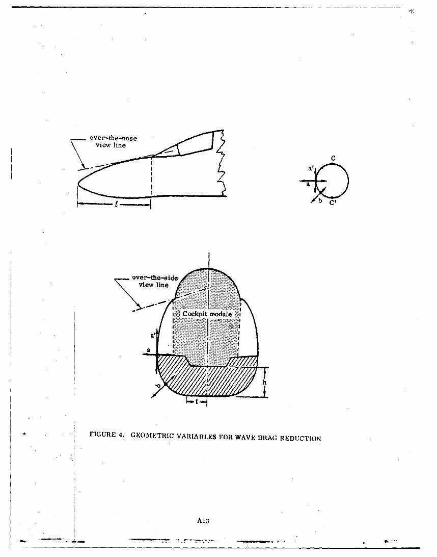
Six geometric variables were selected to generate a family of forvard fuselages
including the F--4 baseline. As illustrated in Figure 4, these variables are the length
; of the fuselage nose, the horizontal displacement a and vertical displacement a' of
the maximum horizontal breadth line. the shape factor b, the lower deck height, h,
and the bottom flat width f. As discussed previously the shape factor b is the distance
from the origin to the 45L tangent line which is tangent to a contour curve of the lower
fuselage cross section. All configurations generated by these variables havethe same
canopy as the F-4 and must satisfy the over-the-nose and over-the-side view line
limitations.
The correspondence between the geometric variables and the reduced variables
defined in Eq. (2), the ranges of variation of these geometric variables, and the base-
line values of these variables are tabulated in Table 2. The variety of configurations
that can be obtained using these geometric variables within their ranges of variation
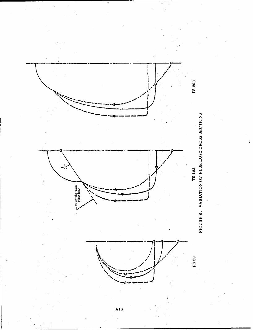
Is illustrated in Figures 5 and 6. Figure 5 shows the top and side views of the con-
figurations. The solid lines show the baseline configuration of the F-4. ..The.dash-dot
lines describe two extreme variations of the fuselage shape. The variation of the fuse-
lage shape ahead of the canopy has to satisfy the over-the-noseview constraint, and
the width of the fuselage is subject to the over-the-side view constraint. The radar
installation Imposes a minimum requirement for the width and limits the amount by
which the lower profile can be moved upward. Notice that the figuire shows only two
extreme examples of the variations. The long nose version can be combined with a
wide fuselage or the short nose version can be combined with a slender fuselage to
yield other intermediate confiivrations. Figure 1; demonstrates the type of configura-
tion variation that can be achieved through the chosen variables. Cross-sectional
views at the three fuselage stations indicated in Figure 5 are shbwn ili Figure 6. The
solid lines describe the baseline configuration while tile dashed lines describe two
extreme variationw o( the cross sections. The circle at F. S. 50, which represents
A12
ovver-the-side
ove i•h noseodil
FIUe 4 EMTI AUBX O AEDA EUTO
eA1I

TABLE 2. VARIABLES, RANGES, AND BASELINE VALUES
Reduced Geometric Ranges of x. Baseline ValuesVariables Variables Ranges 1 xiBaein aleK. xXi. x. z. x.
1min m"max 1 1
11
z 1 84 104 -1.38 87.1
z2 b -2/3 2/3 0 *
z3 f 0. 1.5 2/3 1.
z4 h 5. -10. -2/3 0.
z 5 a' 0.6 1.2 2/3 1.
z a 0.9 1.15 .0.4 1.
*Baseline values for x. vary from station to station. x. is taken,i Im I ni
to be the local baseline value minus 2/3 of the difference between the
baseline value and the local minimum value and x. is taken to be theImaxlocal baseline value plus 2/3 of the difference between the baseline value
and the local maximum value.
A14

Iij III. I
IjIL jfI I
':1 -�
'I, a a -
U z
Ii 2iii I ii 4-LI
Ii r..I.. II -ii' 'I
I 'I
ml* I IIa: ' ii I -ii I I cj�
III II'mm -
I'* II
I Is* 1/
Al !�
- - .s..-.,....- - - - - -- e-------,------- -.. --
I
/ C.,
'I f
- If
"4 =- -- ;'-- -~ .... ...
-. __ _•
- z

the minimum area for the radar, limits the amount by which the maximum breadth line
can move in or the lower profile can move up. The over--the-side view line governs
how far the maximum breadth line can move out and up. Again only two extreme
examples are given. Other configurations can be easily constructed. The important
variable for the cross-sectional variation is the shape factor b which drastically alters
the shape of the lower fuselage between the maximum breadth line and the lower sur-
face flat.
It should be fairly obvious that the choice of geometric variables and their ranges
of variation are somewhat arbitrary. The present selection allows a fairly wide range
of variation of configurations which are similar to the baseline configuration. Other
selections can be made such that the range of variation is more limited or the family
of configurations is less similar to the baseline.
Some guidelines for the selection of geometric variables and their ranges can
be given.
(1) The two linear variables should be selected if their effects on the wave drag
are small or if they affect the wave drag nearly linearly and their interac-
tions with other variables are very small. The interaction between two
variables is the influence of either variable on the wave drag contribution
of the other. Nonlinear effects, however, can be included through a new
concept which will be discussed in Section 4c.
(2) The four remaining nonlinear variables should be selected in such a way
that their interactions with each other are small or nearly linear.
(3) The range of each variable should be as small as necessary, just wide
enough to serve the particular purpose.
(4) In general Lhe nonlinear variables and their ranges should be selected in
such a way that their influences on the wave drag are of the same order of
magnitude.
A17

4. FLOW lH1E:LD CALCULATION AND WAVE DRAG EQUATION
vhe wave drag coefficients of the baseline configuration and the 25 configurations
picked by the Latin Square technique are calculated by applying the Three-Dimensio-ti•
Method of Characteristics. The resulting wave drag coefficients are then u, 'o ob-
tain the wave drag equation.
a. F'low Over F-4 Baseline
As an example of the flow fields calculated by using the Three-Dimensional
Method of Characteristics, the flu.: over the F--I baseline at Mach 2.5 and zero angle
of attack is presented here. F.igure 7 shows the top and front views of the configura-
tion, four cross-sectional views, and the upper and lower centerline pressure distri-
butions. Along the upper centerline of the con figuration. the pressure rises sharply
as the flow hits the canopy-fuselage juncture. This signifies the existence of an
embedded shock wave created by the canopy. At the pressure peak the local Mach
number'drops to 1. 17. As the flow spreads over the canopy flat section, the pressure
drops although the canopy profile is almost straight. A sudden drop of pressure is
experienced as the canopy profile curves back after the flat section. Along the lower
centerline the Cp first drops to a negative value due to further expansion. It recovers
somewhat and eventually comes close to zero, consistent with the condition of zero
angle of attack.
Figure S shows polar plots of the pressure distributions at four fuselage stations
with cross sections shown in Figure 7. Since the forward fuselage ahead of the canopy
droops somewhat, the pressure is higher on the upper fuselage than that on the lower
fuselage at zero angle of attack. At F.S. :35.4 the C incr'ases monotonically from ap
slightly negative value at the bottom to a positive value at the top. A noticeable
'prcssure rise can be seen at F.,S. 85.3 near the fuselage-canopy juncture. A similar
pressure peak is visible at F.S. 145, at which C has become negative except near
p
A1S
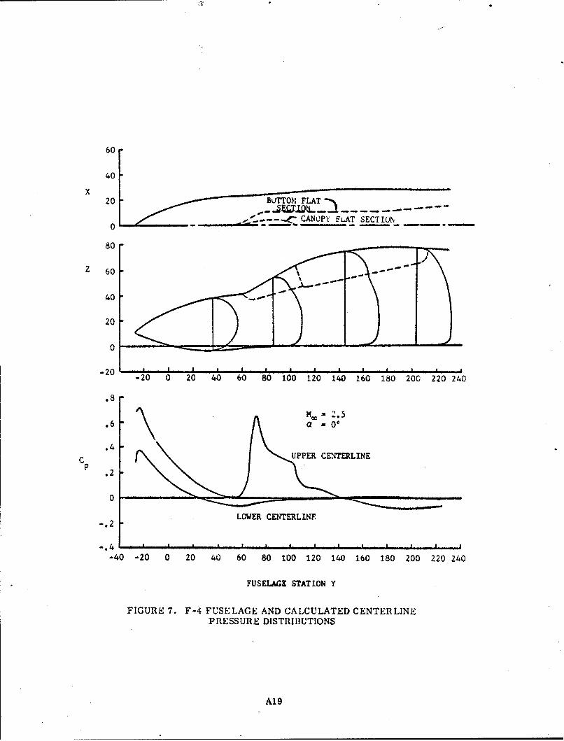
60
40
x 20X BUTTON FLAT " -20
0
80
Z 60
40
20
0
-20-20 0 20 40 60 80 100 120 140 160 180 200 220 240
.8
M•- -2.5.6 al =A 0
.4p .2UPPER CEN,.TnERLINE
p
0
LOWER CENTERLINE-. 42
-40 -20 0 20 40 60 80 100 120 140 160 180 200 220 240
FUSELAGE STATION Y
FIGURE 7. F-4 FUSELAGE AND CALCULATED CENTERLINEPRESSURE DISTRI1BUTIONS
A19

C 0
C =0p
•o 0.4
0.2
0.1
0
(a) FS 35. 4
(b) FS 85.3
V
C =0 I
Positive cp C
S p
(d) FS 203
FIGURIE: 8. POLAR GRAPHS OF PRESSURE DISTIIBUTIONS AT FOURFUSELAGE STATIONS
A20

the bottom flat. In general the flow continues to expand downstream. By F. S. 203 the
pressure everywhere has become slightly less than the free-stream pressure, and the
variation of Cp is small and nearly monotonic.
b. Calculation of Wave Drag Coefficients
As shown in Eq. (1), for a given Mach number and angle of attack, the wave
drag coefficient CDwis assumed to be a quadric function of the six chosen geometric
variables x . . . . x6 with the coefficients a i and aij to be determined. The reduced
variables zi. which take the levels of 0, t1, ;2 according to the Latin Square arrange-
ment shown in Table 1, assign corresponding values to the geometric variables x..
For instance, according to the first cell, z1 and z6 are assigned level -2, which cor-
responds to the minimum values of the geometric variables x1 and x6 while z4 is
assigned level 2, which corresponds to the maximum value of x4' The other three
reduced variables are assigned levels corresponding to intermediate values of the
geometric variables. Thus the first cell specifies a set of values for the geometric
variables which in turn defines a configuration whose wave drag coefficient can then
be calculated by the method of characteristics program. In this way, each cell leads
to one equation for the determination of the ai and aij in the wave drag equation.
Since the method of characteristics is based on hyperbolic equations, the com-
plete flow field must be supersonic in order to apply the method. As mentioned above,
the local Mach number dropped to ". 17 near the fuselage canopy juncture of the F-4
at free-stream Mach 2.5 and zero angle of attack. Local subsonic regions would likely
occur' for some of the 25 variation configurations if the free-stream Mach number
should be lowered. Hence the wave drag coefficients for the F-4 fuselage and the
25 variations, each corresponding to a cell of the Latin Square, were calculated using
the Three-Dimensional Method of Characteristics program at Mach 2.5 and zero angle
A21

of attack. The calculatei wave drag coefficients (based on a wing area of 530 sq. ft.
ar1 tabulated in Table 3. The' mcan value ,4' the 25 coefficients is slightly higher than
the baseline coefficient.
c. Wave l)rag, Equation
In the wave drag equation, Eq. (1), two of the geometric variables, i.e., x and
x 6,1have only linear te rms while other variables have nonlin"r'.,r terms. In this way
there are only 17 coefficients a. and a.. while there are 25 equations available for their
evaluation. It therefore seems logical to include nonlinear terms of x1 and x 6 in the
equation as well. However, a preliminary numerical study suggested that the matrix
of coefficients of the system of 25 equations has a rank of 17 and consequently only 17
unknowns a. and a.. can be determined.
It is more convenient to express the wave drag equation in terms of the reduced
variables z. Since the reduced variables always take the levels 0, :1, :-2, the least
square fitting procedure once developed can be applied to any other values of the
geometric variables without modification. Also. since all reduced variables are of
the same order of magnitude, the coefficient of each term in the wave drag equation
is a measure of the contril)ution of that term to the total wave drag. In terms of the
reduced variables the original wave drag equation takes the form
6 5 5 (13)
CD b= + b~ z+ b..z.z.CDW bo i I bjzz
il j=i i=2
When the coefficients bi and bij were evaluated using the calculated wave drag co-
efficients of the 25 cells and the baseline in a least-square procedure, Eq. (13) was
A22
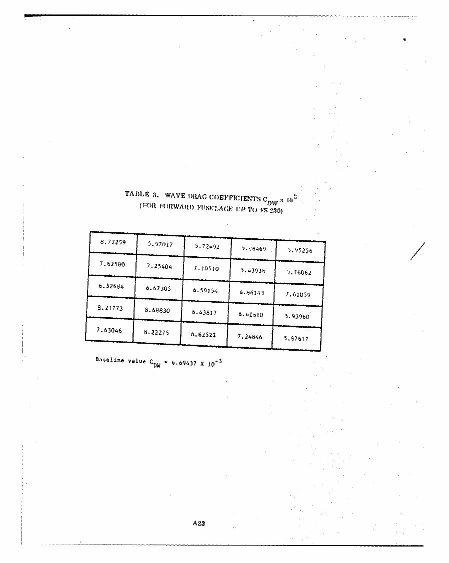
TABLE :. WAVE I)ItAG COEFFICIENTS CDW x 10"(FOR I"ORWAJIt) "USE IA(GE 1 P TO 0Y% 230)
8.72259 5.97017 5."2492 )" 5.95256
7.b2580 7.25404 7.20510 5.4393o 5.76062
6.52684 6.67305 6.59154 6.66143 7,61059
8.21773 8.68830 6.43817 6.61810 5.93960
7.63046 8.22275 8.62522 7.24846 5.876-17
Baseline value C DW 6.69437 X 10⁻³
A23
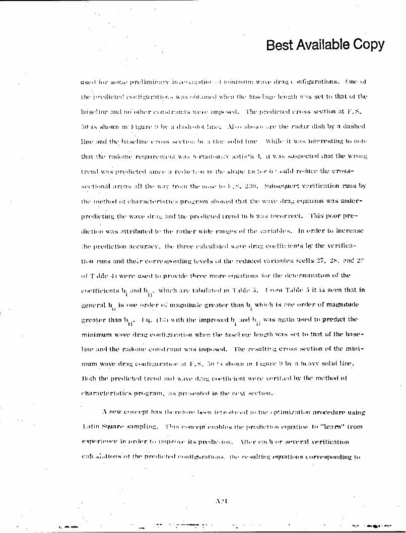
Best Available Copy
used kur si m~c prel.imlin~i 'vinU.:ti' !nummnfim waive alrait L. .rltgrati(ns. O ne (A
the p!-cdict('(' Vt II HIj1. I"Itit 't'\ , ~ l(nt v.1itiz tilt- i i1a4 Ici't-h w~sSet tot that ul the
bais& ine and nott t lu'r van~ ~aa .'r. eaimp-. *st. t'he prtdictud erass soction at F. S.
,)0 -is shaaWnl ill H.-uare !I at d:1 a-t t ý. \. h txn xva .rc th r~ad:ar dish by a daiihed
line( mid the b~aselilna. era 4ss s.ttctiu;; !av : thia stihd lint- \\hilc it W%:is itit~rt'stifl to naotc
thait thle r1ltIl('re4U ranatW 1 0atit''tLX S:ItiSli A. it \:as sasjieetel th~at thle wPIIwg
trenld was tareaietet Sfincc :1 Irc~il *1il inl, th1e 'ha 4 X~ 1) , kuld re''tue the cross-
s&etitmnJ.1 areas :ill tilt- VtV!1 hetise t(' -)..0. Subseq'(uet,'t v:Iitiettiofl Xfs b
the Ilefiethal (,I ha rIcte ri st ics 0r1.ramsh xdthAt th~ i av d r-ia equa u1OD was under-
predlieungt' the wae irtý and tile, jarclieteal rena l it 1) -xas hicetrrect. iThis pwor pre-
ahietoinl was It ributed te the rthe r wxide iraraes (,fI the ý:a riait .vs. lIn order t( [ ceres
:he- jredithie n.aeeu racy, the the acletiated %%:we dr:aj.a,etiiet by the ye ri fie -
tion rm rs and the r c ,rreslum andng levels ,l thet reduced varia alvs icells :27, 2,s. :' il(!~
OIf T abi' -11 were used tot praaviih' three more e((u:itions tatir the aieternainwtion otf the
C' ) tieetts ).;1t1(i 1). .. wiheb :1 re I 1:a(l~e tuta'tIll T thlo. :). J.r: l ITalt.e 5 it is seen th~at in
gene ral b is an atWa rt ler a 4 mantmaitucke gr(eate'r than 1). wh ichl is ,nie otrder of mlatfl ittide
greate r thani 1) W U II:', i % ith thet imipr vud I). anmil 1) i w~as ngjnli usedl tat predict the
mnimum Ifl-li vae drag Cat i.'ratianwhent tile fuse1 l 11 .1 I('It. h~ was 5 wtt to at of thle base -
lint( andl the ratla anc can, -t 1-1 lilt w:a s inip'st se. The' resulti.'g C rilss sectioan ofI the mniti -
mum w~ave alr:ig c4tatti 4u ratt oil ;Iat I,. S. -)0 Slit mil Iln I i-41ure 9t bm a hit :avY Solid linle.
I 1i th the pred icted t rendl :aid t.a ye al':g e'lice iet 'were va'ril ,e IY (lite mel(thod of
c.h~mi acte ristie s tpr'g ran , ;i s prce m'atad ini thet it.a\t sectitait.
A fiew caaa.ea'Pt ha--s thi re0 aa' IN'atl ia'wr' 'l'at-a to, tilt, 'pIimi/imatlt nrm'edure usinig
I :itini Squa ra itnipli iit. This vi'a'nea't ri):ilh's. the( prirelietiai ' nitt vtlm olIl ''lemi"t tIrom
v\Twui'ria'aav in1 istraer I imiaapirao 'itsg pra'die iton. \ fi'r eatt It (r sever~al verirficaition
:I&.:,. Hops 4 Ocl te p~ra'riata'tt ''tt.t1ai~atn ri-4tiltiait ('fithiatais u&aart('mpottdilig tiit

B aASELINE
FICU. 9i. FUSEI.A;F: CIi(SS SECTIONS AT F. S. 50
A25
..- .0 -.
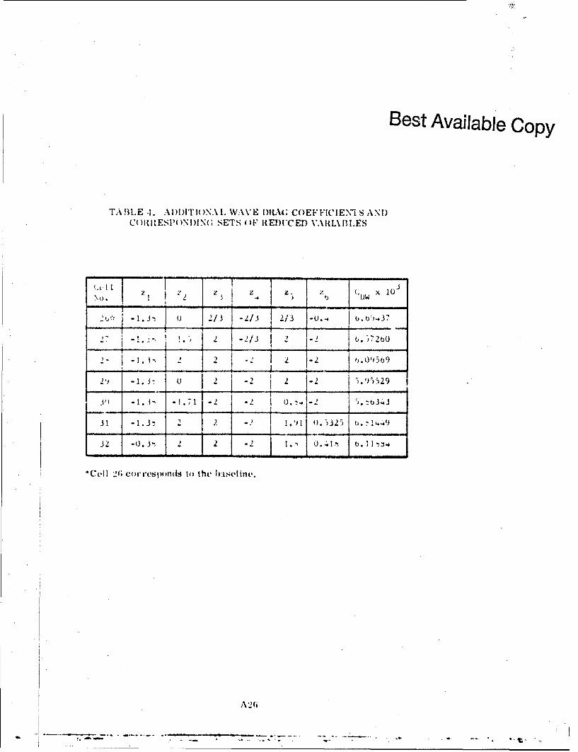
Best Available Copy
T.ABLE-I. AlI)IITIO)N.\L WAV'E I)UAX(CCoEFFIICIENT-S AN!)C( RIRESPO NDI)N(, SETS O)FRIEDUCED \'ARL\ 3.S
IAt z L~ / 10
1/ -2/3 2 1,3 -0-4
2-1 2- 1 -2 7 269
29 -1. 3- 0 j2 j-21 12123') -1.t 17 -2 -2 0.. -2 5. -n343
31 -1.3- - .2 -. 9 0 ,32 4 4
32 -0.3 2 -20.4 ti3
*ccli 26G cor rsponsls to the huisel inc.
A 26
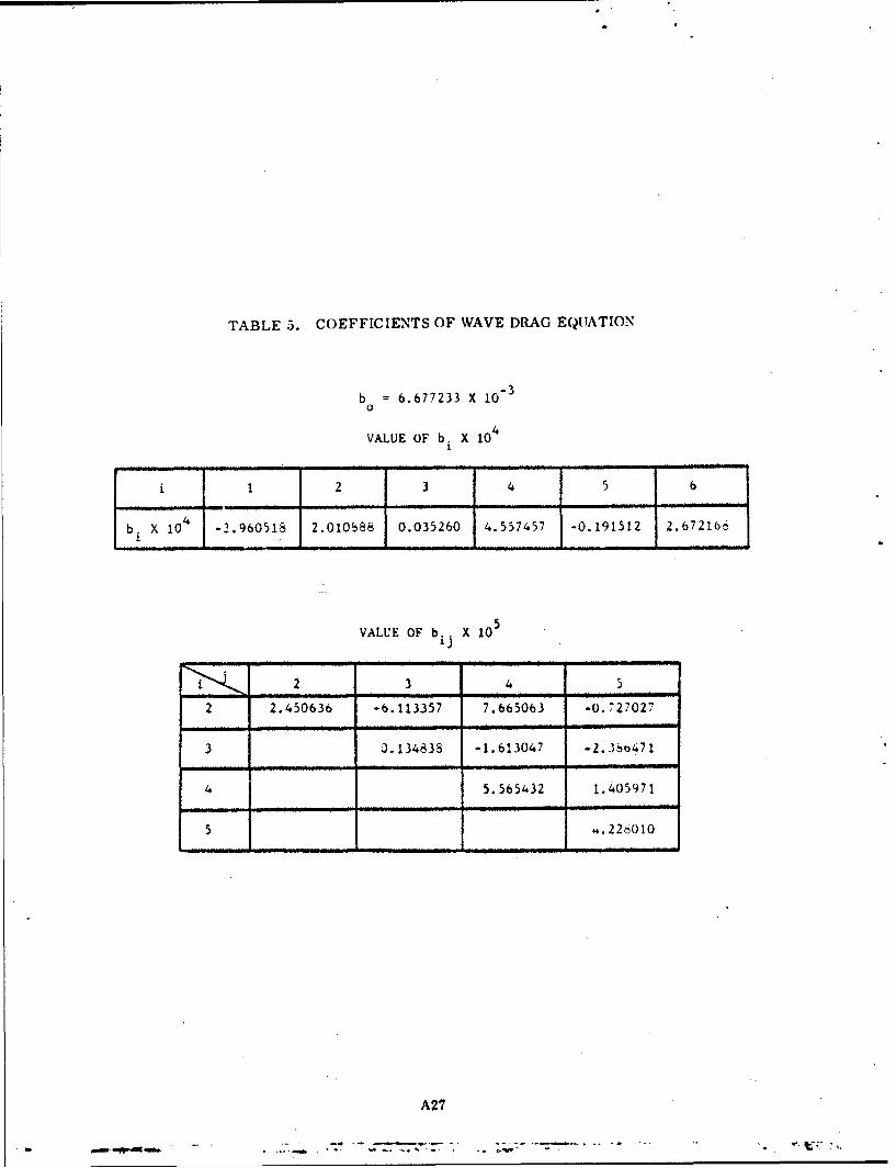
TABLE 5. COEFFICIENTS OF WAVE DRAG EQUATION
b = 6.677233 X 10⁻³⁰
VALUE OF b. X 104I
1 1 2 3 4 5 6
b. X 10 -2.960518 2.010•88 0.035260 4.557457 -0.191512 2.6721b
VALUE OF b.. X 105
2 3 4 5
2 2.450636 -6.113357 7.665063 -0.727027
3 0.134838 -1.613047 -2.3gt471
4 5.565432 1.405971
5 4.226010
A27

Best Available C;...
the \erification rtus are included in the least-square procedure to, obtain improved
coefficients b. and b.. of the prediction equation. In general one or two applicationsI ij
of this process should yield satisfactory results. The improved prediction for one set
of constraints may or may not lead to improvement for other sets of constraints. Ilow-
ever. the same process can be applied wherever needed.
An additional advantagc of this new concept is that nonlinear terms involving z
and z,; can also be taken into account. With each addition of an equation due to a verifi-
cation, the rank of the matrix of coefficients usually increases by one. That means one
more b.. of a nonlinear term involving rZ or z can be included. This process can be
repeated, if necessary, until all quadric terms arm accounted for.
A28

5. GEOMETRIC CONSTRAINTS AND WAVE DRAG REDUCTION
The wave drag equation can now be investigated to reduce the wave drag. In the
process of determining the minimum wave drag configuration. certain geometric
constraints, such as minimum cross-sectional area or maximum fuselage length,
must be satisfied. For each set of geometric constraints there exists a minimum wave
drag configuration. In this section the optimization procedure and some minimum
wave drag configurations are presented and discussed.
a. Optimization Procedure and Geometric Constraints
The simplest and surest way to find the minimum wave drag configuration
subject to a given set of geometric constraints is to use Eq. (13) to calculate the wave
drag coefficients for all allowable sets of levels of t'e variables and pick the set that
gives the least wave drag. The optimization procedure consists of the following,
steps.
(1) Make a numerical search through the ranges of all six variables, using the
wave drag equation to calculate the wave drag coefficients for those sets of
levels that satisfy the constraints.
(2) Identify the set of levels of the variables that yields the least wave drag.
(3) Prepare body description Input data for the minimum %.ave drag configuration.
(4) Use the Three-Dimensional Method of Characteristics program to verify the
wave drag coefficient predicted by Eq. (1I).
The coefficients b. and b of Eq. J13) were obtained by applying a least square
procedure to fit the hypersurface represented by -:q. (13) over the 25 wave drag co-
efficients given in Table :1 and the first four coefficients of Table -t. The standard
deviation of the dt was about 1.02 x 10'4 which corresponds to an error of about 1.517,
The Numerical Search Procedure is presented in Appendix D.
A29
VI'• = . .. . .. - . .-. -. -. * ... .. . . •• . " .77_- .. ' ",
based on the mean wave drag coefficient. The maximum error of the fit over the 29 data
points was about 2.4""'(. Hence step 5 of the optimization procedure is necessary for
wave drag reduction of 4-5"; or less as predicted by Eq. (13).
Four types of geometric constraints are considered in order to satisfy most
design needs. These are:
(1) One or more of the six geometric variables take assigned values within the
ranges of variation. For instance, the length can be kept the same as that of
the baseline or the width can take 90f" of the baseline width.
(2) At one or more fuselage stations the configuration cross sections contain
geometric curves prescribed by tabulated data of widths versus elevations.
This type of constraint is useful for the placement of particular equip-
ment, for instance, the radome.
(3) At one or more fuse!age stations the configuration cross sections satisfy
minimum area requirements. The minimum area can be either a given area
or a certain percentage of the baseline cross-sectional area.
(4) The configuration satisfies a minimum volume requirement between two
given stations. A given volume or a certain percentage of the baseline
volume can be imposed.
b. Minimum Wave Drag Configurations
Several minimum wave drag configuratiGns subject to various geometric con-
Straints are presented to illustrate the application of this program. These configura-
tions were obtained by using the optimization procedure, and the predicted wave drag
coefficients were verified by the Three-Dimensional Method of Characteristics (33DMoC)
program in some cases.
A30

Within the ranges of variation of the six variables (when the only constraint was
implicitly imposed by the ranges under consideration), a 34. 8H reduction of the wave
drag coefficient was predicted by Eq. (13). The configuration corresponds to the
longest nose, as might be expected. \%%ien the length was set to be equal to that of
the baseline, a. 151'( reduction was predicted by the equation. The percentage reduc-
tion of the wave drag in relation to the increase of fuselage length is plotted in
Figure 10. It is seen that for every inch the fuselage is lengthened the wave drag
equation predicts a wave drag reduction slightly- over 1%. Since no constraint other
than the nose length was imposed, these minimum wave drag configurations have the
least cross-sectional areas attainable within the ranges of variation of the remaining
five geometric variables. Consequently these configurations cannot contain the radar
dish which is represented by a dashed circle at F. S. 50 in Figures 6 and 9. When
the fuselage length was set to that of the baseline and the radome constraint was
imposed, the wave drag equation predicted a 14,,'; reduction of the wave drag coefficient.
The cross section of this minimum wave drag configuration at F.S. 50 is shown by the
heavy solid line in Figure 9. It is seen that the lower fuselage cross section barely
contains the radar dish. This predicted trend that the wave drag decreases with the
shape factor b in the neighborhood of this minimum wave drag configuration was
verified by calculations using the Three-Dimensional Method of Characteristics
program. Calculation of the wave drag of this configuration also resulted in a wave
drag reduction of 12.617, which agrees fairly well with the 14' reduction predicted
by the wave drag equation, considering that the standard deviation of the least square
fit is 1. 57. The front view of this minimum wave drag configuration is presented in
Figure 11. which shows the contours of the cross sectiors from V. S. 20 to F.S. 230
at Intervals of 10. The front view of the baseline is presented In Figure 12 for com-
"parison. It is seen that this substantial reduction of the wave drag was accomplished
at the expense of reduced fuselage volume.
A31
"DWCDW Baseline 32
28
24
20
16
Al2
8
4
-4 0 4 8 12 16 20,Ai (INT)
FIGiUE I0. REDUcTION OF WAVE DRAG VS TNCREASE OF FUSELAGE LENGTh1
A3 2

40
30
-to
s.
-10 .,
FIGURE 11. FRONT VIEW OF A MINIMUM WAVE DRAG CONFIGURATIONSATISFYING THIE RADOME REQUII{IE MENT
A33
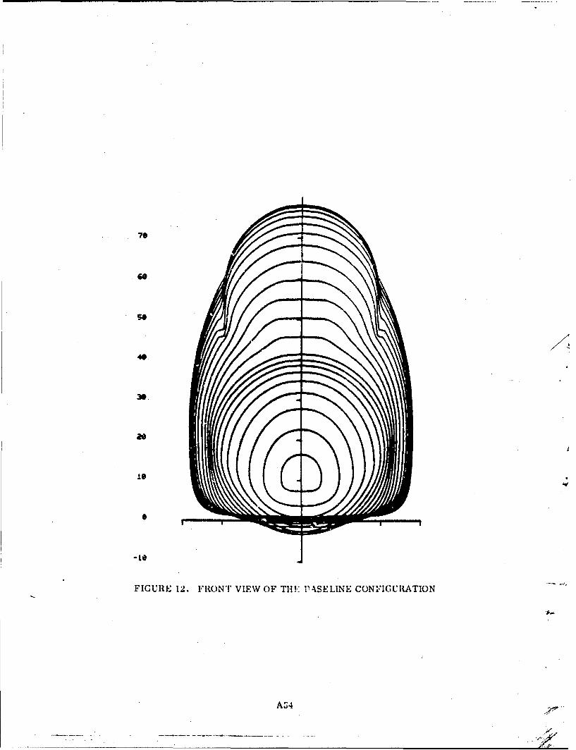
7.
so.
40.
30
-10
FIGURE 12. FRIONT VIEW OF THE' PASELINE CON111GCRATION
A34

Two important general constraints that strongly affect the wave drag are the
fuselage nose length and the fuselage volume. Therefore, the optimization procedure
was used to determine a number of minimum wave drag configurations for various
nose lengths and fuselage volumes. Since the horizontal displacement of the maximum
breadth line has an important effect on the fuselage volume, nonlinear terms of the
displacement a and the nose length I should be included in the wave drag equation for
accurate preaiction of the influence of these two geometric variables on the wave drag.
Equation (13) was first used to obtain two preliminary minimum wave drag configura-
tions which are tabulated in Table 4 as cells 31 and 32. The 30th cell in Table 4 cor-
responds to the minimum wave drag configuration subject to the radome constraint,
which was discussed in the preceding paragraph. These 32 cells provided 32 equa-
tions which allowed 23 terms (or 23 coefficients b , bij ) to be included in an improved
wave drag equation. All important nonlinear terms involving a and I were included.
The final improved wave drag equation, with six additional terms, is expanded
into the form:
CDW b +bZ +b2 Z2 +b3 Z3 + 4 Z4 b5Z5 +b Z
+bz2 2 2 2 2 2 (4+ b11Zl2 + b2 2 Z22 + b3 3 Z23 ÷b 4 4 Z4 2 + b5 5 Z5 + b6 6 Z6 (14)
+b Z Z +b Z Z+b Z Z +b Z Z 4.b Z Z21 2Z1 32Z3 2 41Z4Z1 42 4 2 43Z4Z3
+ 52Z5Z2 + 53Z5Z3 +b 5 4 Z5 Z4 +b 62Z6Z2 +b 64Z6Z4
The coefficients of Eq. (14) are tabulated in Table 6. The optimization procedure using
the improved wave drag equation was then applied to determine the dependence of the
wave drag on the nose length and fuselage volume. The predicted percentage reduc-
tion of the wave drag coefficient is plotted against the increase of the fuselage nose
length in Figure 13 for various fuselage volumes (expressed as ,r of the baseline
volume). The two circles mark the calculated percentage reductions of the wave drag
A35

Best Available Copy
0
r
-0
3' • .J
'0L" , " .O (0 r--
I r
0",
I
I
n
A36

using the Three-Dimensional Method of Characteris-ics for the two Selected configura-
tions. Excellent agreement between the predicted vnd calculated wave drag reduction
is seen. When the nose length and fus:lage volume were set to the baseline values,
very little wave drag reduction was obtained within the variations of the six geometric
variables Is selected. This set of geometric variables and their ranges were chosen
to illustrate the wave drag reduction procedure in such generality that a wide range of
configurations similar to the baseline was covered and various illustrations could be
made. No specific effort was made to tailor the variables to the wave drag reduction
of the baseline configuration. The baseline wave drag could conceivably be further
reduced by some appropriately selected variables. Referring to Figure 13 again, some
rule-of-thumb percentage reductions of the wave drag can be observed. On the average
one inch increase in the fuselage length reduces the wave drag by slightly over one per-
cent while one percent decrease in the fuselage volume reduces the wave drag by about
3/4 percent.
The characteristics of the improved wave drag equation are shown in Figures 14
through 18. Each of th., figures shows the variations of the wave drag coefficient with
respect to two of the six geometric variables, where the remaining four are set equal
to the values of the baseline. Although it is difficult to plot the preser.t wave drag
function in a six-dimensional space, these figures at least enable one to isolate and
study the interacting characteristics between anv two of the six variables. The effects
of volume are also shown by plotting symbols on the curves to indicate various fuselage
volume limits. Since the geometric variable b is different for different fuselage sta-
tions, the parameter b used in these figures is actually the reduced variable which is
constant for each given configuration.
Figures 14a through 14e show the variations of the drag coefficient with respect
to the height of the lower deck h for families of f, b, a', a and f, respectively. Within
the ranges of variables studied, CDW decreases monotonically with h. Figure 14a
A1D7
Best Available Copy,
r
In I
* F!CVIIIK12.- M1'UK1U'1N OSF WAVE.K DI)Ii; VS INCRE~ASE(Sf i9~iK .At 1 LN T ! V VA!ZIM'S *T;SIKLIA(;i;
VmNUI -'01' B:o ASE IANEI VO)LUME')
-iz
VolSymbol VolBL
X .98 f I
.99 a'
aso 1.00 b, baseline
o 1.01
* 1.02
-84
S7
-10.0 -7.5 -. e -8. 0.0 2.5 50
h
r FIGURE 14a. CHARACTERISTICS OF THE WAVEDRAG EQUATION - CDW VS h (FOR CONSTANT 1)
A39
VolSymbol VolBL
X .98 8 7.1
f IA .99
a' I
o 1.00 .a 1
o 1.01
*" 1.02
I I
- 2
I7
.4-10.0 -7?.5 -$.o -$ 00e s. .0
h
FIGURE 141). CIlARACTEP'"TICS OF TlII WAVE DRAG
EQUATION - CDW VS h WFO1 CONSTAN b)
"A40

I JVolSymbol Vol BL
X .98 i-87.1
.99 f I
a'~
O 1.00 b, baseline
o3 1.01
* 1.02
9.0-
aa,
"-1.2
-7.5 -S.0 -2.$ 0.0 a.S 5.0
h
FIGURE 14c. CHARACTERISTICS OF THE WAVE DRAGF EQUATION - CDW VS h (FOR CONSTANT a')
A41

Vol
Symbol VolBL
X .98 2 97.1
A .99
0 1.00 h, baseline
o 1.01
* 1.02
10
.9
.a I . . . . . .
-1.0 -7.5 -;.o -2.5 0..5 5.0
"h
FIGURE 14d. CHARACTE:RISTICS OF Tiii WAVE DRAGEQUATION - CDW VS h (FOR CONSTANT a)
A42
Symbol Vol BL
X .98 -87.1
A .99-- atal
0 1.00 b, baseline
o 1.01 1
1.02
f0
5
8 .
p..
1.5
-- S. -2.5 0.0
h
FIGURE 14e. CHARACTERISTICS OF THE WAVE DRAGEQUATION C CD VS h (FOR CONSTANT f)
A43

Best Available Copy
Lildk ates that for a given jolu me, CI)W decreases w ith the length of ih fuselagte nose
C. Along values of constant vo lurne. Fig'res 141), 14c and l4d show that when each of
the respective variables (b, a' and a) interacts with h, there is a definite combina-
tion of variables which yields a configuration o"t minimum wave drag. For a volume
equal to the baseline value (Vol/'Vtjlll, 1), for example. Figure 1.4) shows that a
minimum occurs near b h 0 which are equal to the baseline values. The occurrence
of the minimum near the baseline configuration verifies the results obtained from the
numerical search where little reduction of wave drag from the baseline was obtained
within the variations of the selected geometric variables. Lines of constant a' and a
in Figures 14c and 14d respectively are nearly parallel, indicating that the interaction
between a' and h and the interaction between a and h are weak. This fact is also
revealed by examining the magnitude of the coefficients of the wave drag equation tab-
ulated in Table 6. The magnitude of these interaction terms, although included in the
• •formulation of the wave drag equation, is one order of magnitude smaller than the
raverage of the remaining interaction terms. Figures 15a and 15b show Lhe varia-
tions with respect to the length of the nose t for families of a' and f. respectively.
Again, the trend shows that C DW decreases with V, but miniria for given constant
volumes are not definitely shown. Figure 15b shows that the width of the fuselage
bottom flat section has little effect on the drag coefficient when the remaining four
variables are set equal to the values of the baseline. Figures 16a through 16d show
the variations with respect to the horizontal displacement of the maximum breadth line
a for families of i, b, a' and f, respectively. Here, the figures show that the drag
coefficient increases monotonically with a. Similar to the results shown in Figures
M-1a through 14le, for constant volume the drag coefficient decreases with f, and when
the volume is equal to that of the baseline, minima occur at or near the ba.seline. In
Figure 16b, for example, the minimum occurs at a -: 1.01 and ) t/6 approximately
for Vol/Vol 1. The curves in Figurcs ltla, lec, and 1fi( are parallel stince inter-HI..
$ action terms 4etween each of the variables with a are not included in the present wave
7. A44
----- --- - - --- ----. -. -.

Vol
Symbol VolBL
X .98 f=
a .99 h 0
al01.00 b, baseline
o• 1.01* 1.02
7 . C.
."•X,,. /-.a' = .6
M 1.0
S12
- 6.0-
I .
"• •0 85 90 95 '0 0
FIGUfIE 15a. CHARACTERlSTICS OF THE WAVE DRAGEQUATION CDW VS (FOR CONSTANT a')
A45

VolSymbol Vol BL
X .98 h 0
S.99 al I
a-•o 1.00 b, baseline
o3 1.01
* 1.02
7 .S -- f • ...... • . . . . .
f -0, .5, 1.0, 1.5
00
4 80 85 90 9 100 105
Fi(;;UiE 15b. CIIA{ACTEItSISICS OF milE WAVE DRIAGEQUATION -- CDW VS f (FOR CONSTANT f)
A,16%JA4

VolSymbol VolBL
X .98 f 1
A .99 h 0a' -= 1
o1.00 b, baseline
o 1.01
* 1.02
10
raa
I .9 .9 .0$ 1.85 1.10 I-IS
FIGURE 16a. ChIARACTERISTrICS Or TIll WAVE DRAGEQUATION - C DwVS a (FOR CONSTANT I)
A47

Sy m boV ol
.98 i b' I Vo
A .99
o 1.01
* 1.02
6.0
e~~ge1 2/3 .0 x1
FI 1. I 'b. C! TA hACT I-AUSTICS OF TIl l WAVE DR)IAGF:QtUAlT! )N -. C D' VS a1 (FOR) CONSTANT 1))
oL)W

VolSymbol Vol BL
X .98 k' 87.1
.99f 1A .99 f
h1.00 I, baiseline
o3 1.01
*- 1.02
8 1.27 .__ _. . . . . . .. . . . . . ... . . .. . . . .. ...._,__ _._.,
7.- - .
0.90 1.g 1.WS 1.10 .1
FI; LRJE I (k*. C(IARACTEMISTICS OF TIE WAVI*: I)IDUGEQUATIrON - Dc VS a d-01 CONSTANT a')
A43
-,, ..• , - ." . -" " . .. . .. r •.

Best Available Copy
h
- I0Inuelifle
7.2SI' ', .
0 1..O
1.0!
i
, • . s ... I .. ...I /.............
II ui: 'i.c1~ cvus'c ' il \VVCIR(' -.i " i'~ • , :i t) .5, t. (). U1. ')
: : . e ..... .. . . ..... . .. . .. t .. .I . . . . .. ..\
SA3i

drag equation. Similar to the results shown in Figure 15b, CI varies little with 1.I)W
Figu, res 17a and 171b show the variations with respect to the vertical displacement o!f
the mxximum breadth line for families of b and f, respectivel". Here, a minimum
configuration for a given volume constraint cannot be determined graphically but a
minimum can he, located for each constant 1) or f. Figure 17a shows that the (Irag
coefficient increases with b, except when a' is INxlow the value of the baseline (a' - 1)
and when b is less than about -l/,3. Figure 17b shows that the drag coefficient in-
creases with f when a' is below the baseline value (a' = 1) and the trend reverses when
a' is above the baseline value. Figures lsa and 18b show the variation with respect to
the shape factor b for families of f and f, respectively. Again, Figure 18a shows that
the drag coefficient decreases with E. Similar to the characteristics of CDW vs. a'
shown in Figure 17b, the trend of the wave drag coefficient reverses from increasing
with f when b is below the baseline value Pi n 0) to decreasing with f above the baselineI
value. Along the constant baseline volume line, Figure 18b shows a slight reduction
of the drag coefficient from the baseline when f 1.5 and b -. 25.
t
1Aix
A51

Best Available Copy
VolSymbol Vol BL
X .98 1 87.1f I
A .99
h 0SO 1.00 a 1
or 1.01
*• 1.02
7?.4-' -
1-~/3. 8
00' • •1/3
S • •__. 2/3
r r
0.6 0.7 0.8 0.9 1.0 1.1 1.2 1.3
FIGURE 17a. CHARAcTrERsITICS OF THE \ WAVW. DRAGP.QUATION - CDW VS a' (FOR CONSTANT h)
A52

VolSymbol VoIBL
,BL
X .98 1 87.1h o.99
aro :1.00 b, baseline
3 1.01
*• 1.02
7.1 - - - .
01.0
00
g.,S
0q .6 0.7 9. .9 1.0 1.1 ".1.2.
., aa
FIGURE 17b. CHARACTERISTICS OF THlE WAVE DRAGI. EQUATION - C VS a' (FOR CONSTANT f)
DW
A53

IVolSymbol V B
X .98 f--
99 .99
o 1.00 a'=
a 1.01
* 1.02
.89
.3 -0).s -0.4 -0.2 0.ý0 0. P 0.4 0. 0.b
FIGURE 18Ma. CHARACTERISTICS oF THE WVAVE DRAGEQUATION - CD VS 1) (FORl CONSTANT J)
I,,w
IA5

•/
VolSymbol Vol BL
"X .98 1-87.1h::4 .99
a' 10 1. o0 a=1
o] 1.01
* 1.02
7. 4 - -.. . -. ... .- p
7.2- ---
x
1. 0 roew
.6..
-0.8 -0.6 -0.4 -0.2 0.o 0. P 0.4 0.6 0.8
b
FIGURE 18b. CHARACTERISTICS OF THE WAVE DRAGEQUATION CnW VS 1) (FOR CONSTANT f)
A55

4 6. CONCLUDING REMARKS
The following remarks and conclusions can be made for Phase I of the wave
drag reduction program.
a. The optimization procedure using the Latin Square sampling technique and
the Three-Dimensional Metlod of Characteristics is useful and practical.
The procedure can be used for other optimization purposes besides wave
drag reduction.
b. The geometric variables"and their ranges of variation should be selected
carefully sinceethe'quality of the procedure and results are affected by the
selection. Some guidelines on selecting the variables and ranges are given
in this appendix, but experience is valuable.
c. A new concept has been introduced to enable the optimization procedure to
improve during the course of determining the optimum configuration. This
concept is particularly useful when the variables and their ranges were not
well chosen either because of inexperience or for the sake of compromise.
d. Within the ranges of variation of the six chosen geometric variables, the
following rule-of-thumb percentage reductions of the wave drag are ob-
tained for the F-4 fuselage. For every inch the nose is lengthened, theI.
wave drag is reduced by slightly over one percent. For each percent the
fuselage volume is decreased, the wave drag Is reduced by about 3/4 percent.
5.A
f
A56

�( i REF ERENC ES
1. Redlich, 0. and Watson, F. R., "On Programs for Tests Involving SeveralVariables," Aeronautical Engineering Review, Vol. 12, No. 6, June 1953,p)p. 51-59.
2. Chu, C. W., "Compatibility Relations and a Generalized Finite-DifferenceApproximation for Three-Dimensional Steady Supersonic Flow," AIAA JournalVol. 5, No. 3, March 1967, pp. 493-501.
3. Chu, C. WV., "A New Algorithm for Three-Dimensional Method of Character-istics," AIAA Journal, Vol. 10, No. 11, November 1972, pp. 1548-1550.
A
2A5
* - - a - - - - , --- -. a - . .- - . .. ' C

APPENDIX B
THE LATIN SQUARE METHOD
1-3The Latin Square is a sampling method for designing an experiment.
AnNth order Latin Square is an arrangement of the N values of N + 1, or fewer,
variables (where N is a prime number) in such a way that the resulting surface
fitting process is efficiently performed. The method may be used for determining
an approximate equation for a function of a number of variables and hence for solv-
Ing extremum problems when the dependent variable is not known as an explicit
function of the independent variables.
The dependent variable, in this case wave drag coefficient CDW, is assumed to
be a quadric function of the independent variables x. (which are related to tht geometry
of the forward fuselage in this application),
6 5 5
!DW a0 + 6 a+ 1 i i i(1=1 =
Equation (1) is written for a 5 x 5 Latin Square with six independent variables, i.e.
r N-5.
.For a given set of independent variables, xV, a new set of reduced variables,
say z1, may be determined such that the variables z take the values 0, *1, 4,
"2 * N-I2--, according to the transformation equation
X +Xa
rThe .5 x .5 Latin Square arrangement in terms of the levels of the reduced
variables Is shown in Table 1. The arrangement may appear to be at once regular
A Bi

and random. It appears to be regular since all variables take orderly permutated
values. It appears to be random since there seems to be no bias in representing
all segments of the population. Regularity and randomness - therein lies the ef-
ficiency of the Latin Square sampling technique. It has been shown by Yates 3
that randomized blocks are more efficient than complete randomization and Latin
Squares are more efficient than randomized blocks. fie also found that on one set
of experiments about 2 1/2 times as many plots were needed with the randomized
blocks of 5 blocks as with the 5 x 5 Latin Squares to obtain the same accuracy (see
Reference 1, pp. 202-203). Careful examination of Table 1 revealed that in all
the cells having a given level of any reduced variable any one of the remaining
variables takes on all possible levels once and only once. For example, if we
select z1 = -2 to be the given level of the one reduced variable, then column
one contains all cells having z1 -2. It is seen that in column one each of the five
levels of any one of the remaining variables, say z2, appears once and only once.
Consequently, the number of all cells having a given level of any reduced variable
is five since there are five levels for each of the other variables to take through a
permutation process. Several consequences can be observed. Firstly, if we com-
pare any two cells we find that only one of the variables has the same level in both
cells, whereas all other variables have different levels. Secondly, for each re-
t duced variable there are five groups of five cells which satisfy the condition that in
each group this reduced variable takes one of the five levels. Thirdly, by a suitable
rearrangement of the cells any pair of the reduced variables can take the column and
row indices as their levels just as z1 and z(; (do as shown in Table 1. To do this,
arrange each group with the same level of one variable as a column and arrange the
columns In an ascending order with respect to the levels of this variable. Within
&,, each column (or group) arrange the cells In an ascending order with respect to the
ADM.

TABLE 1. A 5 x 5 LATIN SQUARE ARRANGEMENT
CELL CODE z2 z5
-2 -2 -1 -2 0 -2 1 -2 2 -2
1 0 2 1 -2 2 -1 -2 0 -1
-1 2 0 -2 1 -1 2 0 -2 1
-2 -1 -1 -l 0 -1 1 -1 2 -1
2 -1 -2 0 -1 1 0 2 1 -2
1 0 2 1 -2 2 -1 -2 0 -1
-2 0 -1 0 0 0 1 0 2 0
-2 -2 -1 -1 0 0 1 1 2 2
-2 -2 -1 -1 0 0 1 1 2 2
-2 1 -1 1 0 1 1 1 2 1
-. 2 0 -2 1 -1 2 0 -2 1
0 1 1 2 2 -2 -2 -1 -1 0
-2 2 -1 2 0 2 1 2 2
" 0 1 1 2 2 -2 -2 -1 .1 0
2 -1 -2 0 -11 0 2 1 -2
4 B
B3

Best Available Copy
levels of the other vari:able of the pAir. These properties show heuristicatllv the.
efficiency of the Latin Squire s-.mplin- technique which has been used for develop-
4-5ing various optimal designs.
It may seemn intricaite to constcuct a Latin Square of this type, especially when
the size exceeds 5 x 5. The following steps, however, van be followed to construct
this type of Latin Square of any size "s long as the number of rows (or columns) is a.
prime number. The steps are best explained using Table 1 as an example.
(a) The variables z and Z,; are assigned levels equal to the column. and row
indices :as shown in Table I.
(b) For each of the diagonal cells where 4 z the level of z. is inc.reased
Isuccessively from i 1 to i (i by a level equal to that of z in a cyclic
order, in which the lowest level (i.e.. -2ý is considered one level higher
than the highest level (i.e., 2).
(c) The remaining levels of z., to z. iii each row are obtained by permutation
in an increasing cN-clic order using the diagonal cell.
References
1. Kempthorne, 0., The Design and Analysts of Experiments, Wiley, New York, 1952.
2. Redlich, D. and Watson, R. F., "On Programs for Tests Involving SeveralVariables," Aeronautical Engineering Review, Vol. 12, No. 6, June 1953.
3. Yates, F., "Complex Experiments," Suppl. J. Roy. Stat. Soc., Vol. 2, 1953,pp. 181- 247.
4. Powers, S.A., "Minimum Drag Bodies of Revolution by Exact Methods,"* NOR 63-159, Northrop Corporation, September 1963.
5. Powers, S.A., "Drag Minimization Using Exact Methods," AIAA Journal,
May 1964.
4
b B4
-.. ... .. . . .. -T#,t.t• .. •. .. •,• .. • . •'m
APPENDIX C
BODY DESCRIPTION METHOD
In this Appendix, the general body description method is described in some
detail and is illustrated by the body description of phase I. The technique of fitting
a conic-section curve is also given.
The fuselage is described by a number of generating lines, such ab the upper
profile, the lower profile, the maximum half-breadth line and generating ines for
the canopy. In the present body description procedure, each generating line is
divided into as many segments as necessary to allow each segment to be described
by a conic-section curve. At each cross section of the fuselage simple analytic
curves, e.g., the ellipse or cubic, connect any two adjacent generating lines to
form the contour of the cross section. The fuselage is thus described analytically
by simple low order curves.
The body description procedure detailed here was developed for use in con-
junction with the three-dimensional method of characteristics for calculating flow
fie!ds over smooth bodies. For a smooth body a unique normal to the surface must
exist every where, and this condition of a unique normal usually requires that the
curves and their slopes be continuous at the juncture between two contour curves
or two segments of a generating line.
1. DEFINITION OF GENERATING LINES
The fuselage is located in a right-handed coordinate system where the Y-axis
is aligned with the fuselage axis, the X-axis is spanwise and the Z-axis is up. A
schematic of a fuselage-canopy configuration is shown in Figure 1 and a typical cross
section in Figure 2.
In general, five generatinv lines, each being described by two functions of Y
(representing their vertical and horizontal projections Z and X , respectively, by a
general curve fit of conic sections) plus an additional three lines, each being
described by a single function of Y. serve to define the fuselage-canopy configuration
in phase I.
Cl

z
Canopy Sill
(•)-
Canopy Sill
"FIGURE 1. ýACIIEMATIC OF :ITSELACE-CANOPY CONFIGURATION
• o2

Best Available Copy
z0
K FIGURE 2. TYPICAL FUSELAGE CROSS SECTIONVC3
7.C.

Best Available Cel,
Thcse are identified in Figures I and 2 as C ,Q tpper profilc line(a M\l•imum half-hreadth liae
(D Lower profile lineQ• Canopy crown line
() Canopy definition line
® Shape factor b, locating the 45* tangent line
® Upper fairing line
) ILower fairing line
where lines Q(E), 0, (), are required only, of course, in the region of the canopy.
The conic-section curves describing the lines take the form
(U)- Py + Qt [R.5Y .T]+ (1)
Details of the determination of the coefficients P, Q, R, S, T of the general conic
curves will be discussed in Section 4. Each conic-section segment must be con-
tinuous with the previous segment and, with very few exceptions, the slope must be
continuous at the junctures to satisfy the requirement of a unique normal to the sur-
face discussed above. Unlike others, line Q is not a true generating line. It is
actually a shape factor for the lower part of the fuselage, which expresses the dis-
tance to a tangent line as a function of Y. A lull discussion of the details is pre-
sented in Section 2(c).
Lines (S and (9 which fix, at each cross section, the extent of the fairifig cubic
between canopy .nd upper fuselage are defined by their projections in the YZ-plane,
i.e. Zf,01 and Zf 2(Y), only. Their projections Xf,(Y) and Xf 2(Y) are constrained
to lie on the ellipses defining the canopy and upper half of the fuselage, respectively,
ais deta'it.. in Section 2(d).
2. CONTOUR CURVES FORMING CROSS SECTIONS
As shown in Figure 2, for the most general case of a fuselage-canopy coitfiguratlon
with a windshield flat, the contour of the cross section begins with a straight line
representing the flat from the centerline to . The canopy contour froh (D to ®
is circular, but can be elliptic in general. The upper fuselage is represented by an
elliptic curve between (a and Q. The lower fuselage is represented by a general
C4

coMic-section curve from ® to . the bottom flat by a straight line from ® to the
centerline. The intersection between the canopy and the fuselage is faired by a cubic
from - ®0 to 0.
a. Canopy
The cross-sectional shape of the canopy is assumed to be circular. If there is no
winidshield flat, ( will lie on the centerline (Figure 3a) and the equation for the
canopy curve is given by
Z. 2 =#.-( 1 .0 (2)
If a windshield flat does exist, 0 moves off the centerline as shown in Figure 3b and
Equation (2), describing the canopy between ® and 0 leads to a slope discontinuity
at (D, the juncture between the circular arc and the windshield flat. Thus, a quarter-
ellipse is used to approximate the circular arc between ( and Q to give a slope of
dZ/dX = 0 at Q, providing slope continuity with the flat portion of the contour. TheI ~equation for this approximating ellipse is
a2
0 .N .1 (3)
The details of determining the point 0, given the locations of the canopy crown and
sill lines, exre presented in Section 3.
b. Upper Fuselage
The equation for the upper fuselae is
-- 4-- (), 0 (4)
indicating that, for the body description in its present form, X is constrained to be
zero for all Y.
Again it may be noted that (), in the region of the canopy, is fictitious and cannot be
obtained directly from three-view drawings. Details of determining Q, given the
location of the maximum half-breadth line (5 and the location of the canopy sill line,
may be found in Section 3.
C5

N
I -
� N
UN
- 0X N
U *- N CI)II -0�-
z
* *
CI)
0z
U 0N
0n N CI)
N__________
I N 0
N
* x
pI.
7. C6

c. Lower Fuselage
Referring to Figure 2, the contour curve from () to Q) has a zero slope at Q) and
the slope approaches infinity at (a. As in aircraft lofting practice, the shape of this
contour curve is determined by specifying the distance from the origin to one of its
tangent lines that makes a 45* angle With the X-axis. Hence, this distance, which is
designated by b in the following derivation of the equation for the contour curve, may
be regarded as a shape factor for this curve.
The equation for the 45* tangent line is
z. x-r b
which, when the origin is translated to ( becomes
Z' M x' + (5)
where Z'= Z-Zm, X'= X- Xm and H Xm -Zm 2 b. In the new coordinate system, the
the general quadric equation, satisfying the conditions X'(Zl) X!, Z'( 0) 0,
(bX'/aZ')m = 0 and (OZ'/aX')1 = 0, reduces to
K(x z'-Z XT)+ x'(t- P) - 0 (6)
which represents a family of curves with K as a parameter. To determine K, Eq. (5)
is substituted into Eq. (6) to yield a quadratic equation of the form
AX' ÷8x' - 0(7)
The condition for Equation (6) to be a tangent line is that Equation (7) have a double
root; i.e. B~- 4AC - 0, which leads to
K . ...- (8)
Equation (6) with K given by Eq. (8), then represents the contour curve from 0) to (®).
The range of variation of this curve obtainable by applying this equation is illustrated
in Figure 4, where a family of conic section curvw is given for different values of b.
By increasing the distance b, the curve is seen to vary from almost a straight line
to a sharply bending curve approaching the two sides of a right triangle.
C7

f6
4
272 b 7 6
K8 6
! ~~9.5--/• \\fF 4 A AMILY OFCOI
-'2 4 6 10I
I7.
2 8.0 -Sb 9.0
4
" FIGURlE 4, A FAMvLY OF CONIC-SECTION CURVES
I1.,
, d. Fairing Curve
The intersection between the canopy and upper fuselage is faired by a cubic from Gto (D. The projections Zf,(Y) and Zf2 (Y) of lines ©D and ®D on the YZ-plane are given
by conic-section curves (such as Equation (1), where P, Q, R, S, T are input quantities).
The projections Xf,(Y) and Xf,(Y) on the XY-plane are obtained by solving Eqs. (3) and
(4), respectively.
XI,(Y') . (X.x-xC)[1-I(lfi"-oal
(9)
Xf,,Y) - X .,- ,Z.rnJ" , '/ I
The fairing curve matches the slopes of the ellipses at both end points fi and f2. The
slopes are defined by differentiation of Eqs. (3) and (4)
b • (Y) = zf- zg C !(4o- - (10)Ox o Y) • .,, )( )_
___ ZIA IV
The cubic equation that satisfies the conditions of Eqs. (9) and (10) at point ft. can be
written
x .÷ P.11(Z-Zf) ÷ + Oxf, Z_.2j R.L.f& (11E/' al Zf.-Zft" Zf- aft"
// .
The coefficients c and d are obtained by applying the conditions of Eqs. (9) and (10)
at point f2
,C• 3(X,,- x,,) Z( a,• l )(,,,- Zf),C r (12)
" Id -z(Xt,-x.t)÷ (MI bxf-) (z,,- Zf,)
Equation (11) with c and d given by Eq. (12) is then the cubic equation for the fairing
curve from (E) to (D. The quantities Xfl, Xf2, OXf,/OZ, DXf2/OZ are given by Eqs. (9)
and (10), while XfI. Xc, X#. Zu, Zm, ZO, Zf1, and Zf2 are obtained from the genera-
ting lines input in the form of Equation (1).
•9:. ~C9
S *- . * -.-.

3. D)ETERMINING GENERATING LINES AS FUNCTIONS OF Y
The g-enerating lines defined in Section 1 are determined primarily by utilizing top
and side view drawings as well as available cross-sectional views. The top and
side views arc used to obtain the variation of generating lines Q and 0) in the
A Z-plane and of line o in the XY-planc. The variation of line (3 in the YZ-plane
und of line ® in the XY-planc are obtained primarily by utilizing cross-sectional
views, as is the description of the shape parameter (D as a. function of Y.
From Figure 2 it can be seen tliat line Q, in the region of the canopy, and line ®are, in effect fictitious lines whose description three-view drawings will not yield di-
rectly. The two iines are determined by assuming that the cross section of the canopy
is a circular arc and by constraining the intersection of this circular arc and the ellipse
defining the upper portion of the fuselage to lie on the canopy sill line, which in turn is
well defined from available three-view drawings.
In Figure 3, let Xi, Zi be the location of the canopy sill line for the cross section
shown. Utilizing the general equation for an ellipse with center at X0 , Zo and semi-
major and minor diameters a and b, respectively,
+ ( Z 20 ) 2 0\b
one may determine Zu by finding b in the above equation for the ellipse through the
point Xi, Zi with known center X0 = 0, Zo - Zm and a X", yielding
Zu . 4 X. (Z Z"i)(13)
To determine Z# and X#, defining one end point of the quarter circle passing through
Zc, X€ and Zi, Xi whose center lies on X0 - 0. it is necessary to obtain Zo and r
for the circle satisfying the following conditions
x!* (+ -Z.) (14a)
* (LZ.) r (14b)
* Solving for Zo yields
1., W Zoo (15)
I . - -. -C IO-. . ... .
• •:,• -.4 • *- . . . ... .......-.

and using Equation (14b) to solve for r, gives
x. - r - + " Z' -Zo)1 (16)
When a windshield or canopy flat exists (i.e. Xc *•0, as shown in Figure 3b) a slope
dis-ontinuity results at Xc, Zc. Thus, for Xc * 0, the circular arc is replaced by
a quarter-ellipse, passing through Xi, Zi and one end point being XC, Zc with dX/dZ =0
to provide slope continuity.
This ellipse is intended to be an approximation to the circular arc determined previous-
ously. It is obtained by decreasing the canopy flat (i.e. Xc) by an arbitrary percen-
tage and solving for a new Z# and X# by an iterative procedure. utilizing Zo and X0
of Eqs. (15) and (16) as a first approximation, while constraining the product of the
two semi-axes of the ellipse to be equal to r2 of the initial circular arc.
Given a tabulation of Xc, Zc, XmI Zm, and Xi, Zi, values of Zu, Zo and Xo can be
determined for a number of fuselage stations; their fit by a sequence of conic-section
curves as a function of Y can then be accomplished in a straightforward manner by
the techniques described in the following section.i
4. EVALUATION OF THE COEFFICIENTS FOR A CONIC SECTION
The general equation of the second degree, which represents a conic section, is
t2 bxtl c .a (17)
utilizing the coordinate system of Figure 5. The general equation appears to have six
constants, but in reality has only five arbitrary constants, since Equation (17) can be
divided by any of the constants, leaving an equation with five undetermined coefficients.
Therefore five independent conditions are sufficient to determine a conic.
In the following sections, two ways in which these five independent conditions arc
supplied will be treated. Section 4(a) deals with the conic determined by five points,
no three of which are collincar. Section 4(b) treats the conic determined by one point
and two point slopes. By a point slope it Is meant that a point is given and the slope
R •of the curve at the point is also given.
I."isCl
S... ... .. ..
2. a. Conic Determined bIy Five Points
Consider the problem of finding the equation of a conic through five given points, no
three of which are collinear. Let the points be 1, 2, 3, 4, 5 as shown in Figure 5a.
Then,
Y 0y"r% x -h 2 - 0 (18)y~-mn~x -hi 3 = 0 1IsY-Mt x -h 4 - 0!
represent the equations of the lines connecting points 1-4, 1-2, 2-3, 3-4, respectively.
Then the equation
K (-' X -,HI )(Y -M 3x -h3) + (V-l 2x -h? )(U-rn4 X -h.4 0 .(19)
represents the family of conics through the points 1, 2, 3, 4. In this equation, K is a
parameter whose value can be determined from the fifth condition, which is that the
conic pass through point 5. (If point I is substituted into Equation (19), the result is
identically equal to zero since point 1 was used to evaluate the coefficients m, h, and
Sin 2 , h2 . The same argunent holds for points 2. 3, 4.)
-. S (Y"2zXs -h;)( y•- rx 5 -"h,,) (20)(ys -m, xs - hf)( y- msxs - h3)
After expanding Equation (19) and collecting like powers, comparison with Equation (17)
shows that
a- K.!
b- -[K (m ,ms) + m2 #m 4
K 0. 3 Km *rn,3 m 4 (21)
d - -IK(h 1 .#i3 ) * hat #ih I.4 a.. K(mths+. MshI) + mzh4 + Mn~A
'*Ir. f- Khlhs + hzh4
Rewriting Equation (17) in the form
,ay.4(b d) y +CX +e f -)
9 and solving, using the quadratic formula, yields
y -(bx+d) 1-[(bx+d)Z-4a(cx- ax+*0)l"Za
t ' C12

1Y
Y~ ~~3 h3 4,h
MI, hl
(a) Five Points
m/
"i X"
x(b) Point and Two Point Slopes
FIGURE 5. DETERMINING CONDITIONS FOR CONIC
C13
*,.. .. . . . . . . . . . . . .. . . .. j - • •.- ......

X d..x.i Vx + b~ 1 2 bdx.d - (4acx1+4acY. +4af)1/2AZa L 4a 4az
y - ~ ~ 2X +~ ±(Cx.~ i2 2~ ) 2(2b . _x _d t. b'. 26 ÷,iX _ Y += ex* fl2a 2a t 4.a' a
which can be recognized as Equation (1), with
P - - b/2a
Q - - dI2a
R - Pz- C/a (23)
S - -Pd/a - c/a
T - Q0- f/a
and the sign of the radical to be determined by evaluation.
b. Conic Determined by a Point and Two Point.Slopes
Now consider the problem of finding the coefficients of a conic determined by one point
and two point slopes. This establishes a curve that is tangent to a given line at a given
point, is tangent to another line at a given point and passes through a third given point.
This particular manner of determining a conic is especially suitable since it allows
for specification of slope continuityat the two end points of the conic-section segment,
wnile the great latitude afforded by the third point (control point) in fixing the shape
of the curve is utilized to good advantage in obtaining a good approximation to the data
to be fitted.
Compare Figures 5a and 5b. The points I and 2 of Figure 5a coincide in Figure 5b,
and the points 3 and 4 of Figure 5a coincide in Figure 5b. The line which joins pointsF,
2, 3 and the line which joins points 4, 1 in Figure 5a therefore coincide in Figure 5b.The lines 1-2, and 3-4 of Figure 5a become tangents to the conic in Figure 5b. Thus,
it can be seen that the special conditions applying to Equation (21) are mn i m3 and
h, h3, and the constants for the comic may be written as
a K m 4
C . KmI * mm. (24)
d 1 [2Kh ÷h 2 . h.1
a- 2Kmhi .Amzh, # m4 h2
S , Kh Jhh,
C14
S: a-,• : .. .. .. ... -. 7 • -'.T. "" :. ... . " ""- .. ... -- '.... .... "
wh. ,'c the value of K is now given by
(Y5 -m 2x 5 -hz)(ya- n, xI- h4 ) (25)
(YS x MA, )
The coefficients P, Q, R, S, T for the conic in form of Equation (1) may now be
cowli)utod by using Eq. (25) and Eq. (24) in Eq. (23).
c. Special Forms
TN%,, special forms of Equation (1) are worth noting due to their frequent utilization
in t uis body description procedure.
A straight line has the coefficients
Q - conAnt
R,, *,T O- 0
A circle of radius r., with its center at x., y., has as its coefficients
P 0
Q
R - -A
T r*- -Co
C15
APPENDIX D
NUMERICAL SEARCIH FOR MINIMUM PROCEDURE
The numerical search procedure to determine the miniinum wave drag configura-
tion involves the computation of wave drag coefficients of a large number of discrete
points blanketing the entire region in the six-dimensional space hounded by the given
ranges of variables. The point which has the lease wave drag is taken to be the mini-
mum wave drag configuration. The accuracy of locating the minimum is th, :'efore
dependent on the resoltuion of the numerical network. Accurate location of the mini-
mum can be obtained efficiently by a search-by-steps technique where the search is
first conducted using coarser grids to determine an approximate location, and ther
repeated in a smaller region centered around the location of the previously obtained
minimum. This process cao be repeated as many times as needed to obtain the
desired accuracy. The major advantage of such a numerical search procedure is that
the given constraints can be satisfied easily by merely rejecting points which violate
the constraints during the search.
The searching procedure is summarized as follows:
1. Select the ranges of search by specifying the lower and upper limits of
each of the six reduced variables:
(ZL) , (z) J ,
"2. Select the resolution for each of the variables by specifying the numlers
of node points N (j -- 1,6) of that variable. The rcsoi•tit~w is given by
Z
resolution --N .1
Dl

Best Available Copy
tThe tot:al nuihtlr ol pints for v:10i1 •ea:rch cYcle is equ:il to the product of
t Nil i.V.
S~6total point.-;
j= 1
lFt" ex:ianpile, if 10 point.s :irc s'petifitd for :1 variables, the total number of points
:.1 ('Ciipute th, . six t:il ,es of V:;rial' ls:
i 1, N.
(zi)i .z 1) (ZN ) j . 1, 6I,(z L); N~)
4. At every possible combination of the six variables,
evaluate the given constraints (e. g. the volume). If the combination satisfies the
constraint, compute the wave draag coefficient using the wave drag equation.
5. Determine the set of variables z'. which yields the least wave drag co-
efficient. The configuration defined hr z' z 2, .... 2 z', is the mini-
mum wave drag configuration unless one wishes to impr6ve the accuracy by
repeating the search.
6. If the search is to Ix, repeated, select the new ranges ofithe six variables
," by redefining the lower and upper limits as,
(zi) z (zr) - Z. j .
'4 where 4 are arbitrary increments of zjseiected to definei a smaller
region of search. In situ:itions where zL) or u.) de.fned by the above
ID•. D2_

relations are Ixeond the ranges of consideration, they are. then set equal
to the minimum " L" maximum accordingly.
7. Repeat the procedure from step (2) until the desired accuracy is obtained.
D
f.,
*
*.,
. D3
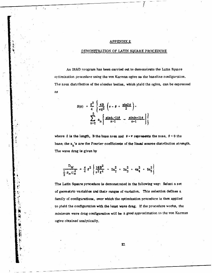
APPENDIX E
DEMONSTRATION OF LATIN SQUARE PROCEDURE
An IR&D program has been carried out to demonstrate the Latin Square
optimization procedure using the von Karman ogive as the baseline configuration.
The area distribution of the slender bodies, which yield the ogive, can be expressed
S' aS
S(a) 4 -B ( s e2)+
* a~ sin(h1)9 -- sin(n-l)f
* where I is the length, B the base area and 9 r represents the nose, 9 0 the
base; the an's are the Fourier coefficients of the lintal source distribution strength.
The wave drag is given by
*D W 7r2 16B 2 2 +32 + 24+5a
lp* U2 14 T2f4 2a 2 + 3a 3 414 5a5 i
The Latin Square procedure is. demonstrated in the following way: Select a set
of geometric variables and their ranges of variation. This selection defines a
family of configurations, over which the optimization procedure Is then applied
to yield the configuration with the least wave drag. If the procedure works, the
minimum wave drag configuration will be a good approximation to the von Karman
ogive obtained analytically.
Elilk

For the 5x5 Latin Square, the six variables and their ranges ace:
x 1 .962 1 f - 1.038
x2 .055 i B ; .079
x3 -. 02 $ a2 _ .02
x4 -. 01 1_ a 5 .01
x5 -. 02 1 a4 g .02
x6 -. 02 L a. 9 .02
The family of 25 configurations defined by these variables is shown in Figures 1
and 2, where the dotted lines represent the base line at I = 1.0 and B = 0.067,
which were selected to reflect the variables used for the F-4 during phase I study.
The demonstration of the Latin Square procedure and our finds are sum-
marized below. A straightforward application of the original Latin Square pro-
cedure did not yield the correct minimum wave drag body. Under the constraint
of given length (I= 1.0) and base (B = 0.067), the original procedure predicted
the minimum wave drag body to correspond to a2 = -. 02, a 3 .02, a 4 -. 002
and a5 -. 02 while for the von Karman ogive all the a's vanish a 2 = a.3 a 4 =a 5 0.
" Of these four variables only a4 is barely acceptable, considering the numerical
accuracy. However, when the iterative type improvement, which consists of
"adding more nonlinear terms in the wave drag function (see Reference 1 of the
main tect), was applied, the optimization procedure turned out successfully.
Indeed, when only one case of a2 = 0, a 3 & 0.2, a4 = 0 and a5 0 was added to
yield a square term for a3 in the wave drag function, the improved procedure
predicted the minimum wave drag body to correspond to a2 = -. 00026, a3 -. 00021,
a 4 z 00006, a5 . 00031, which is the von Karman ogive recovered numerically.
E2
il___

il" 0
DI
lip.
E3 .

- 0
'. ~E4 "
I -.

Similar results were obtained for different constraints of I and B.
In sum,- the improved Latin Square optimization procedure has numerically
predicted the minimum wave drag body that was obtained analytically.
S.1
I;
23• .i•.Best Available Copy
L
FE.
-'-7