Distributed Load Balancing over Directed Network Topologies

Alejandro Gonzalez-Ruiz and Yasamin Mostofi

Cooperative Network Lab

Department of Electrical and Computer Engineering

University of New Mexico, Albuquerque, New Mexico 87131, USA

Email: {agon,ymostofi}@ece.unm.edu

Abstract— In this paper we consider the problem of dis-tributed load balancing over a directed graph that is not fullyconnected. We study the impact of network topology on thestability and balance of distributed computing. We furthermorepropose Informed Load Balancing (I-LB), an approach in whichthe nodes first reach an agreement over the balanced state,through using a consensus-seeking protocol, before proceedingto redistribute their tasks. We compare the performance of I-LB with that of the Original Load Balancing (O-LB) approachin terms of speed of convergence and bandwidth usage. Weprove that the O-LB approach can guarantee convergence toa balanced state as long as the underlying graph is stronglyconnected while I-LB may not converge. However, I-LB canincrease the speed of convergence and/or reduce the bandwidthusage especially for low-connectivity graphs.

I. INTRODUCTION

Everyday there is an increasing demand for high perfor-

mance computing. High speed networks have become more

common, allowing for interconnecting various geographi-

cally distributed Computational Elements (CEs). This has

enabled cooperative operation among the nodes, which can

result in obtaining an overall better performance than the one

achieved by a single CE. Grid-computing is an example of

a system that can benefit from cooperative computing [1].

Distributing the total computational load across available

processors is referred to as load balancing in the literature.

The goal of a load balancing policy is to ensure an optimal

use of the available resources so that each CE ends up with a

“fair” share of the overall job, thus allowing the overall load

to be completed as fast as possible. Load balancing can be

implemented in a centralized [2] or a distributed manner [1].

In this paper, we are interested in distributed load balancing,

where each node polls other processors in its neighborhood

and uses this information to decide on a load transfer.

There has been extensive research in the development

of effective load balancing policies. In [3]–[6] various dis-

tributed load balancing schemes that use concepts such as

queuing- and regeneration-theory have been proposed and

analyzed. A common factor in these approaches is that the

amount of load to be exchanged is based on the weighted

averages of the loads of the neighboring nodes. In [7]–[9] the

proposed policies use concepts such as graph coloring and

gossip algorithms. These algorithms do pairwise balancing

This work was supported in part by the Defense Threat Reduction Agencythrough grant HDTRA1-07-1-0036.

of loads, i.e. two adjacent nodes are randomly chosen to

exchange their loads at a given time step.

In the load balancing literature, a common assumption

is to take the topology of the underlying graph to be

undirected. However, most realistic wireless networks will

have asymmetric uplink and downlink, resulting in directed

graphs. This is due to the fact that wireless transmissions

in uplink and downlink typically occur in two different and

uncorrelated pieces of bandwidth [10], resulting in different

and uncorrelated link qualities. Furthermore, different nodes

may have different transmission power resulting in different

reception qualities (even if the links were the same) and as a

result directed graphs. Another scenario where the network

topology is directed occurs when there are firewalls between

certain nodes that allow incoming connections but block

outgoing ones. Therefore, in this paper we mainly focus on

directed graphs. We study the impact of network topology

on the stability and balance of distributed computing. For the

case of a one-time arrival of the loads, we show that load

balancing over a strongly connected graph reaches a balanced

state independent of the initial load distribution while having

a spanning tree is not a sufficient condition for reaching

a balanced state. We furthermore propose Informed Load

Balancing (I-LB), an approach in which the nodes first reach

an agreement over the global balanced state before starting

the actual load balancing process. We show that while I-LB

lacks asymptotic performance guarantees, it has the potential

of increasing the speed of convergence and/or reduce the

bandwidth usage especially for low-connectivity graphs.

The paper is organized as follows. Section II presents

our system model. Section III explores the impact of graph

topology on distributed computing. Section IV shows the

asymptotic convergence of the distributed load balancing

algorithm to the balanced state. Section V introduces I-LB,

an alternative load balancing approach, and explores the

underling tradeoffs between I-LB and the original load

balancing approach. We conclude in Section VI.

II. PROBLEM FORMULATION

Consider a distributed computing system of n nodes

connected over a wireless network with a directed topology

that can be described by a graph G = (N, E), where N is

the set of nodes N = {1, ..., n} and E is the set of edges

2009 American Control ConferenceHyatt Regency Riverfront, St. Louis, MO, USAJune 10-12, 2009

WeC13.5

978-1-4244-4524-0/09/$25.00 ©2009 AACC 1814

connecting the processors. Let xi(k) represent the load on

processor i at time k ≥ 0. The goal is to spread the subtasks

among all n processors as evenly as possible such that no

node is overburdened while other nodes are idle. At every

time step the nodes assess how overburdened they are and

exchange loads in order to increase the overall computational

efficiency.

For the purpose of mathematical analysis, we take the load

of each processor to be infinitely divisible such that xi(k)can be described by a continuous nonnegative real number.

We furthermore assume that: (i) tasks are independent so

that they can be executed by any processor; (ii) processors

are homogeneous, i.e. they have the same processing speed

and (iii) the link-level delay in the exchange of loads between

nodes is negligible. This last assumption is justified when the

product of the queue length and the service time (execution

time per task) is considerably greater than the time it takes

to transfer a group of tasks from one node to the other.

We also assume that processors are synchronized, i.e. all

the processors perform load balancing at the same time. As

indicated in [11], assuming synchrony yields similar results,

in terms of the final load distribution, to the ones obtained

by working with asynchronous algorithms.

A. Link Symmetry

Consider the wireless link from node j to node i and

that from node i to node j. In wireless communication,

these two transmissions typically occur at two different and

uncorrelated pieces of bandwidth [10]. As a result, the link

quality in the transmission from node i to node j can be

considerably different from that of the transmission from

node j to i, resulting in an asymmetry. Therefore, in this

paper we take G to be a directed graph. Then a neighborhood

set Ni of node i is given by all the nodes j ∈ N such

that there is a directed link from i to j. In other words,

Ni = {j ∈ N |(i, j) ∈ E} with |Ni| representing its

cardinality.

The nodes furthermore exchange their queue lengths with

their neighbors continuously in order to assess how over-

loaded their local neighborhood is. Since this information

has a considerably lower volume than the actual loads, it

can be transmitted over a separate lower bandwidth channel

or with higher transmission power. As a result, it can

experience better reception quality and higher probability

of symmetry. Therefore, in this paper we assume that the

queue length information is transmitted over an undirected

version of graph G. We are currently working on relaxing

this assumption.

B. Description of the Distributed Load Balancing Algorithm

Let sij(k) denote the load that node i sends to node j at

time k. Let Ji(k) and Ci(k) represent the number of external

tasks arriving to node i and the number of tasks serviced by

node i respectively at time k. We will have the following for

the dynamics of the queue length of node i:

xi(k + 1) = xi(k) −∑

j∈Ni

sij(k) +∑

j∈{l|i∈Nl}

sji(k)

+ Ji(k) − Ci(k). (1)

Using an approach similar to the one presented in [1] and [3],

the amount of load to be transferred from node i to node jcan be calculated based on the excess load of node i. Define

avei(k) as the local average of node i, i.e. the average load

of node i and its neighbors:

avei(k) =1

|Ni| + 1

xi(k) +∑

j∈Ni

xj(k)

. (2)

Note that although the graph for the exchange of loads is

directed, we assumed an undirected graph for the exchange

of queue length information. Therefore the ith node has

access to the value of xj(k) for all j ∈ Ni and can therefore

calculate its local average.

The excess load of node i at time k (Lexi (k)) is then given

by the difference between its load and local average:

Lexi (k) = xi(k) − avei(k)

= xi(k) −xi(k) +

∑

j∈Nixj(k)

|Ni| + 1. (3)

This quantity represents how overloaded node i is with

respect to its own neighborhood. Next, node i evaluates how

overloaded its neighbors are with respect to its local average.

Let Lexj(i)(k) be the excess load of node j with respect to the

neighborhood average of node i, namely:

Lexj(i)(k) = xj(k) − avei(k) for j ∈ Ni. (4)

Lexj(i)(k) represents how overloaded the jth node “appears” to

the ith one, based on the partial information available at the

ith node. It can be easily verified that∑

j∈{Ni∪ i} Lexj(i)(k) =

0, with the convention that Lexi(i)(k) = Lex

i (k). Define pij(k)

as the fraction of Lexi (k) to be sent from node i to node j.

Then we will have the following for sij(k), the amount of

load that the ith node sends to the jth one at the kth time

step [3]:

sij(k) = pij(k) (Lexi (k))

+, (5)

where (x)+ = max(x, 0) and:

pij(k) =

{

Lexj(i)(k)

∑

l∈Mi(k) Lexl(i)

(k) j ∈ Mi(k)

0 otherwise(6)

with

Mi(k) = {j|j ∈ Ni, avei(k) > xj(k)}. (7)

In other words, node i will send part of its excess load to

node j at time k only if xj(k) is below avei(k).

1815

III. IMPACT OF NETWORK TOPOLOGY ON

DISTRIBUTED LOAD BALANCING

In order to motivate the mathematical derivations of the

next section, we first consider the impact of different network

topologies on distributed load balancing through simulations.

Two concepts that are frequently used throughout the paper

are that of spanning trees and strongly connected graphs. A

directed graph has a spanning tree if there exists a node that

has a directed path to all the other nodes [12]. Furthermore,

a strongly connected graph is a directed graph that has a

directed path from every node to every other one.

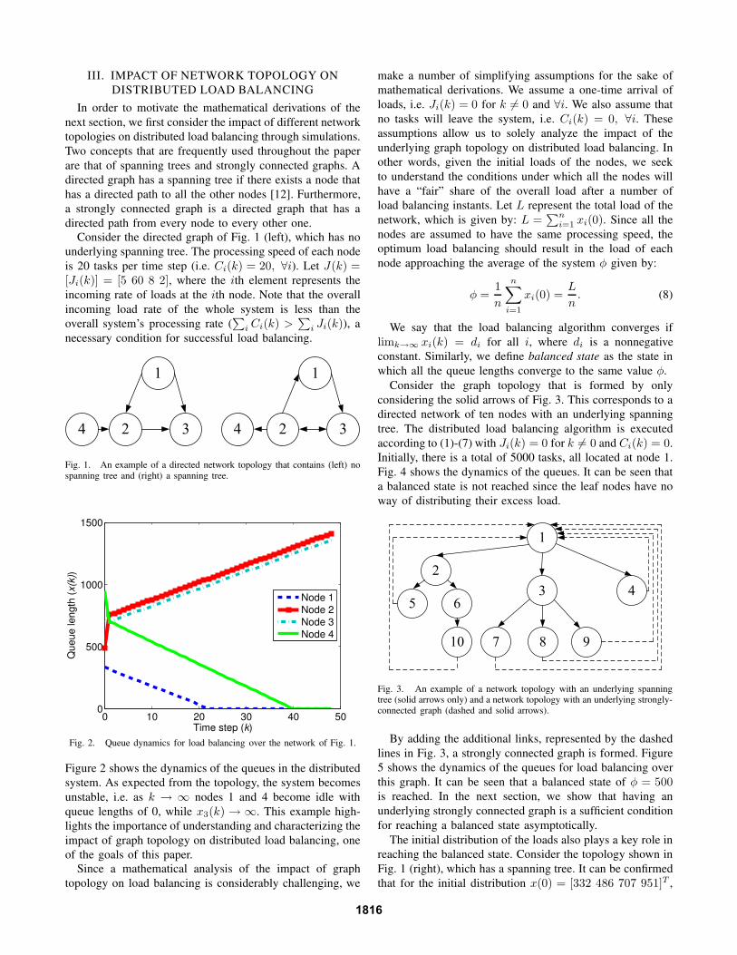
Consider the directed graph of Fig. 1 (left), which has no

underlying spanning tree. The processing speed of each node

is 20 tasks per time step (i.e. Ci(k) = 20, ∀i). Let J(k) =[Ji(k)] = [5 60 8 2], where the ith element represents the

incoming rate of loads at the ith node. Note that the overall

incoming load rate of the whole system is less than the

overall system’s processing rate (∑

i Ci(k) >∑

i Ji(k)), a

necessary condition for successful load balancing.

Fig. 1. An example of a directed network topology that contains (left) nospanning tree and (right) a spanning tree.

0 10 20 30 40 500

500

1000

1500

Time step (k)

Queue length

(x(k

))

Node 1

Node 2

Node 3

Node 4

Fig. 2. Queue dynamics for load balancing over the network of Fig. 1.

Figure 2 shows the dynamics of the queues in the distributed

system. As expected from the topology, the system becomes

unstable, i.e. as k → ∞ nodes 1 and 4 become idle with

queue lengths of 0, while x3(k) → ∞. This example high-

lights the importance of understanding and characterizing the

impact of graph topology on distributed load balancing, one

of the goals of this paper.

Since a mathematical analysis of the impact of graph

topology on load balancing is considerably challenging, we

make a number of simplifying assumptions for the sake of

mathematical derivations. We assume a one-time arrival of

loads, i.e. Ji(k) = 0 for k 6= 0 and ∀i. We also assume that

no tasks will leave the system, i.e. Ci(k) = 0, ∀i. These

assumptions allow us to solely analyze the impact of the

underlying graph topology on distributed load balancing. In

other words, given the initial loads of the nodes, we seek

to understand the conditions under which all the nodes will

have a “fair” share of the overall load after a number of

load balancing instants. Let L represent the total load of the

network, which is given by: L =∑n

i=1 xi(0). Since all the

nodes are assumed to have the same processing speed, the

optimum load balancing should result in the load of each

node approaching the average of the system φ given by:

φ =1

n

n∑

i=1

xi(0) =L

n. (8)

We say that the load balancing algorithm converges if

limk→∞ xi(k) = di for all i, where di is a nonnegative

constant. Similarly, we define balanced state as the state in

which all the queue lengths converge to the same value φ.

Consider the graph topology that is formed by only

considering the solid arrows of Fig. 3. This corresponds to a

directed network of ten nodes with an underlying spanning

tree. The distributed load balancing algorithm is executed

according to (1)-(7) with Ji(k) = 0 for k 6= 0 and Ci(k) = 0.

Initially, there is a total of 5000 tasks, all located at node 1.

Fig. 4 shows the dynamics of the queues. It can be seen that

a balanced state is not reached since the leaf nodes have no

way of distributing their excess load.

Fig. 3. An example of a network topology with an underlying spanningtree (solid arrows only) and a network topology with an underlying strongly-connected graph (dashed and solid arrows).

By adding the additional links, represented by the dashed

lines in Fig. 3, a strongly connected graph is formed. Figure

5 shows the dynamics of the queues for load balancing over

this graph. It can be seen that a balanced state of φ = 500is reached. In the next section, we show that having an

underlying strongly connected graph is a sufficient condition

for reaching a balanced state asymptotically.

The initial distribution of the loads also plays a key role in

reaching the balanced state. Consider the topology shown in

Fig. 1 (right), which has a spanning tree. It can be confirmed

that for the initial distribution x(0) = [332 486 707 951]T ,

1816

0 2 4 6 8 10 120

500

1000

1500

2000

2500

3000

3500

4000

4500

5000

Time step (k)

Qu

eu

e le

ng

th (

x(k

))

Node 1

Node 2

Node 3

Node 4

Node 5

Node 6

Node 7

Node 8

Node 9

Node 10

Ideal

Ideal load per node

Fig. 4. Queue dynamics for distributed load balancing over the graphtopology of Fig. 3 (considering only the solid arrows). The queues cannotreach a balanced state even though there is an underlying spanning tree.

0 2 4 6 8 10 12 14 16 18 200

500

1000

1500

2000

2500

3000

3500

4000

4500

5000

Time step (k)

Qu

eu

e le

ng

th (

x(k

))

Node 1

Node 2

Node 3

Node 4

Node 5

Node 6

Node 7

Node 8

Node 9

Node 10

Ideal

Ideal load per node

Fig. 5. Queue dynamics for distributed load balancing over the stronglyconnected graph of Fig. 3 (considering both solid and dashed arrows). Thequeues reach a balanced state.

there will be no convergence to a balanced state as the

final values are [332 596.5 596.5 951]T . Consider the same

graph but with the following initial distribution x(0) =[951 707 486 332]T . As seen from Fig. 6, the system reaches

the balanced state. This example shows the impact of the

initial load distribution on the convergence to the balanced

state.

IV. CONVERGENCE TO A BALANCED STATE

In [13] it was shown that a distributed load balancing

algorithm converges to a balanced state if it complies with a

number of conditions. While those conditions were described

with an undirected graph in mind, they can be easily extended

to distributed load balancing over directed graphs. In this

part we show, following a similar approach to [13], that

distributed load balancing according to (1)-(7) converges to

the balanced state. First, note that our load balancing policy

satisfies the following properties:

0 5 10 15 20 25 30300

400

500

600

700

800

900

1000

Time step (k)

Qu

eu

e le

ng

th (

x(k

))

Node 1

Node 2

Node 3

Node 4

Ideal

Fig. 6. Queue dynamics for distributed load balancing over the networkof Fig. 1 (right), which is not strongly connected but has a spanning tree.The distributed system reaches the balanced state for the initial distributionof x(0) = [951 707 486 332]T .

Property 1: If xi(k) > avei(k), there exists some j∗ ∈ Ni

such that avei(k) > xj∗(k) and sij∗ (k) > 0.

Property 2: For any j ∈ Ni and any i such that xi(k) >xj(k) and avei(k) > xj(k), the following can be easily

confirmed:

xi(k) −∑

l∈Ni

sil(k) ≥ xj(k) + sij(k). (9)

If xi(k) ≤ avei(k), Eq. (9) is obvious. If xi(k) > avei(k),the validity of this property is based on the fact that:

Lexi (k)/

∑

l∈Mi(k) Lexl(i)(k) ∈ [−1, 0]. Therefore,

xi(k) − Lexi (k) − xj(k) − sij(k)

= −Lexj(i)(k) −

Lexj(i)(k)

∑

l∈Mi(k) Lexl(i)(k)

Lexi (k) ≥ 0.

Let m(k) be defined as: m(k) , mini xi(k).

Lemma 1: There exists some β ∈ (0, 1) such that

xi(k + 1) ≥ m(k) + β(xi(k) − m(k)), ∀i ∈ N. (10)

Proof: We will follow an approach similar to the one in

[13]. Without loss of generality, fix a processor i and a time

step k. Also consider the set Wi(k) = {j|j ∈ Ni, xi(k) >xj(k)} and denote its cardinality as: |Wi(k)|. From (1) and

(9), we have:

xi(k + 1) ≥ xj(k) + sij(k) ∀j ∈ Wi(k).

Adding over all j ∈ Wi(k):

|Wi(k)| xi(k + 1) ≥∑

j∈Wi(k)

xj(k) +∑

j∈Wi(k)

sij(k). (11)

By noting that sij(k) = 0 if j /∈ Wi(k), we will have:

∑

j∈Wi(k)

sij(k) =∑

j∈Ni

sij(k) ≥ xi(k) − xi(k + 1). (12)

1817

Combining (11) and (12) will then result in:

|Wi(k)| xi(k + 1) ≥∑

j∈Wi(k)

xj(k) + xi(k) − xi(k + 1),

which is equivalent to:

xi(k + 1) ≥|Wi(k)|

|Wi(k)| + 1m(k) +

1

|Wi(k)| + 1xi(k)

= m(k) +1

|Wi(k)| + 1(xi(k) − m(k))

≥ m(k) +1

n(xi(k) − m(k)),

which proves the inequality with β = 1n

.

Consequently, we will have the following lemma:

Lemma 2: The sequence m(k) is upper bounded by L and

is nondecreasing. Therefore it converges.

Proof: From (10) we can easily see that xi(k + 1) ≥m(k), resulting in m(k + 1) ≥ m(k). Since Ji(k) = 0 for

k 6= 0, m(k) ≤ L. Therefore it converges.

In [13] the following lemma is proved which establishes

a lower bound on the queue length of any node j that can

be reached from node i by traversing l edges. Since our load

balancing algorithm satisfies properties 1 and 2, we will have

the following lemma:

Lemma 3: Consider node i. For any node j that can be

reached from i by traversing l edges, and for any k ≥ k0 +3ln, we have

xj(k) ≥ m(k0) + (ηβk−k0 )l(xi(k0) − m(k0)), (13)

where η is a nonnegative real number and β is as defined in

Lemma 1.

Proof: See [13].

Using the previous lemmas, we can extend the conver-

gence proof of [13] to the following:

Theorem 1: (Convergence of the load balancing policy

to the balanced state) Consider the algorithm described in

Section II. If the graph G is strongly connected, then

limk→∞

xi(k) = L/n. ∀i ∈ N (14)

Proof: Consider a strongly connected graph. Then for

a given node i, every other node is at a distance of at most

(n − 1) from i. We can apply (13) and follow the proof in

[13] to conclude that the difference between the highest load

and the minimum load of the system (maxi xi(k) − m(k))has to converge to 0. From Lemma 2 we have that m(k)converges to a constant c. Therefore, limk→∞ xj(k) = c for

all j. Since∑n

i=1 xi(k) = L, we have c = L/n.

V. DISTRIBUTED LOAD BALANCING WITH A

PRIORI KNOWLEDGE OF THE BALANCED STATE

(I-LB)

In the distributed load balancing algorithm of the previous

sections, the nodes have to constantly distribute their “per-

ceived” extra loads in order to reach a balanced state. Since

the loads can have very large sizes, this can result in a con-

siderable use of the available bandwidth. If the nodes could

first reach an agreement over the global balanced state, it can

potentially reduce the overall time to reach the balanced state

and the overall bandwidth usage. In this section we propose

Informed Load Balancing (I-LB), a modification to the

Original LB algorithm (O-LB) of the previous sections. The

main idea of I-LB is to let the nodes exchange information

about their queue lengths and reach an agreement over the

global average before starting the redistribution of actual

tasks. After reaching consensus over the global average, the

nodes start exchanging tasks by comparing their own load

with the global average (φ) instead of the local average

(avei(k)). I-LB has the potential of reducing unnecessary

transmissions and as a result the overall bandwidth usage.

In this part, we compare the performance of I-LB with the

O-LB approach and explore the underlying tradeoffs.

A. Discrete-Time Consensus Problem

In consensus problems, a group of nodes try to reach an

agreement over a certain value (average of the initial queue

lengths in our case). They exchange information with their

neighboring agents and update their values according to a

given update protocol. Define yi(k) as the status of node iat the kth instant of the consensus process. We have yi(0) =xi(0), ∀i ∈ N . The network is said to be in consensus if

yi = yj for all i, j. When each yi = 1nΣjyj(0), the team

has reached average consensus [14].

B. Consensus over the Global Average and Informed Load

Balancing

Let A = [aij ] represent the adjacency matrix of the

underlying graph with aii = 0 and aij > 0 if there exists a

directed edge from node j to node i. The Laplacian of the

graph is then defined as L = [lij ] with:

lij =

{ ∑n

k=1,k 6=i aik, , j = i

−aij , , j 6= i

Let y(k) be the information vector y(k) = [y1(k)...yn(k)]T .

The discrete-time consensus protocol will then be [14]:

y(k + 1) = (I − ǫL)y(k), (15)

where ǫ ∈ (0, 1/maxilii) and I represents the identity matrix.

In our case, it is desirable that the network reaches average

consensus which corresponds to the system average (φ). In

[14], it was proved that (15) can achieve average-consensus if

the graph is balanced and strongly connected. Larger values

of ǫ can furthermore increase the convergence rate. Since we

assumed that queue lengths were exchanged over undirected

graphs in the previous section, we assume the same here for

fair comparison. Once the nodes reach consensus and switch

to redistributing the tasks, we take the graph over which they

exchange the tasks to be directed.

Once consensus is reached, the redistribution of tasks

starts. We have the following modifications to the original

algorithm: Lexi (k) = xi(k) − φ, Lex

j(i)(k) = xj(k) − φ and,

Mi(k) = {j|j ∈ Ni, φ > xj(k)}. Eqs. (5) and (6)

remain unchanged. In practice, each node has to switch to

exchanging loads after it senses that consensus is reached. In

order to do so, it could monitor its value (yi(k)) and those of

1818

its neighbors and declare that consensus is reached if those

values do not change over a given time.

C. Underlying Tradeoffs Between O-LB and I-LB

In this section we explore the underlying tradeoffs between

O-LB and I-LB in terms of speed of convergence, bandwidth

usage and performance guarantees.

For I-LB, we take ǫ = 1/(1.1 maxi lii), which will

guarantee convergence. We also assume that the nodes can

detect accurately when the consensus state is reached in order

to proceed to redistributing loads.

Consider the undirected path network of Fig. 7, with an

initial load distribution of x(0) = [707 486 332 951]T . If no

information exchange is done, 49 load balancing steps are

required to reach the balanced state whereas for I-LB, 23

time steps are first required to reach consensus followed by

2 load balancing steps.

Fig. 7. Network topology of a path network. I-LB can reach a bal-anced state considerably faster for an initial load distribution x(0) =[707 486 332 951]T .

I-LB, however, does not always take fewer iterations than

O-LB. As an example, consider the graph of Fig. 1 (left)

with the directed links replaced by undirected ones. Let the

initial load distribution be x(0) = [707 486 332 951]T . If

O-LB is used, the system reaches the balanced state at time

k = 15. For I-LB however, it takes 21 time steps to reach

average consensus and 2 load balancing steps afterwards to

reach the balanced state.

Figures 8 and 9 show a comparison of O-LB and I-LB

for various configurations of an undirected network with 4

nodes and initial load x(0) = [707 486 332 951]T . The two

approaches are compared in terms of speed of convergence

(number of time steps required to reach the balanced state)

as well as bandwidth usage. The figures also indicate the

second smallest eigenvalue of the underlying graph Laplacian

as an indicator of the connectivity of each graph. The larger

the second smallest eigenvalue is, the higher the graph

connectivity will be. In Fig. 8, the bars representing I-LB

include the time steps required to reach average consensus

plus the actual load balancing steps required to get to the

balanced state. By comparing the last two rows, it can be seen

that for graphs with lower connectivity, I-LB can perform

considerably better than O-LB in terms of the total time steps

required to reach the balanced state. However, as the graph

connectivity increases, O-LB can outperform I-LB.

Next we compare the bandwidth usage of O-LB and I-LB.

By bandwidth usage we mean the total number of packets

that are transmitted in the network. We assume that each unit

of task requires 10 times the number of packets required for

transmitting the queue length information of a node. Figure

9 shows the corresponding bandwidth usage of I-LB and O-

LB for the initial distribution x(0) = [707 486 332 951]T

and various configurations of an undirected network with

Fig. 8. Comparison of the time steps required to reach the balanced statefor various network topologies using O-LB and I-LB with 4 nodes.

Fig. 9. Comparison of the bandwidth usage (total number of transmittedpackets) required to reach the balanced state for various network topologieswith 4 nodes.

4 nodes. In most cases I-LB results in a better bandwidth

usage. The difference will be more notable as the ratio of

the size of task packets to information packets becomes

larger. It should be noted that the second column of Fig.

8 and 9 corresponds to the graph of Fig. 7 while the first

column is for the same graph but with a different ordering

of the nodes. As a result, the nodes experience different

loads in their neighborhood. It can be seen that this results

in different performances, which highlights the impact of

the initial distribution of the loads over the network on the

overall behavior.

D. Lack of Asymptotic Performance Guarantee for I-LB

While I-LB has the potential of reducing the time and/or

bandwidth required for reaching the balanced state, it lacks

asymptotic performance guarantee. In section IV, we showed

that load balancing according to (1)-(7) and over a strongly

connected graph can guarantee convergence to the balanced

state. For I-LB, however, this is not the case. We show this

1819

with a counterexample. Consider the path network of Fig. 7,

but with a different initial distribution x(0) = [20 19 20 17]T .

If no information exchange is done, i.e. O-LB is performed,

the system reaches the balanced state, as proved by Theorem

1 (see Fig. 10). However, for I-LB, although the system

reaches consensus, it is not able to reach the balanced state

as seen in Fig. 11. To understand this, consider node 1 and

2. At k = 0, node 2 is already balanced but node 1 is still

overloaded and can only balance itself with node 2. Since

node 2 already reached the global average φ, it is not a

candidate to receive any load, which results in the system

not reaching the balanced state. Intuitively, we can see that

as long as an overloaded node has a neighbor whose queue

is below the global average, it can still reach the balanced

state. The initial distribution of the loads, therefore, plays a

key role in the asymptotic behavior of I-LB.

0 5 10 15 2017

17.5

18

18.5

19

19.5

20

Time Step (k)

Qu

eu

e L

en

gth

(x(

k))

Node 1

Node 2

Node 3

Node 4

Ideal

Fig. 10. Queue dynamics for load balancing over the topology of Fig. 7with no information exchange. The queues reach a balanced state.

0 0.5 1 1.5 217

17.5

18

18.5

19

19.5

20

20.5

21

Time Step (k)

Qu

eu

e L

en

gth

(x(

k))

Node 1

Node 2

Node 3

Node 4

Ideal

Fig. 11. Queue dynamics for I-LB over the graph of Fig. 7 and withx(0) = [20 19 20 17]T . The queues cannot reach the balanced state.

VI. CONCLUSION AND FUTURE WORK

In this paper we considered the problem of distributed load

balancing over a directed graph that is not fully connected.

We studied the impact of network topology on the stability

and balance of distributed computing. For the case of a one-

time arrival of the loads, we showed that load balancing over

a strongly connected graph reaches a balanced state, indepen-

dent of the initial load distribution, while having a spanning

tree is not a sufficient condition for reaching a balanced state.

We furthermore proposed Informed Load Balancing (I-LB),

an approach in which the nodes first reach an agreement over

the global balanced state before proceeding to redistribute

their tasks. We explored the underlying tradeoffs between

I-LB and the Original Load Balancing (O-LB) approach.

While I-LB lacks asymptotic performance guarantees of O-

LB, it can increase the speed of convergence and/or reduce

the bandwidth usage especially for low-connectivity graphs.

We are currently working on extending our results to the

cases with continuous incoming and outgoing loads. A

further extension could include considering communication

delays as well as heterogeneous processing speeds.

ACKNOWLEDGEMENTS

The authors would like to thank Dr. Majeed Hayat and

Jorge Pezoa for useful discussions.

REFERENCES

[1] S. Dhakal, “Load balancing in communication constrained distributedsystems,” Ph.D. dissertation, University of New Mexico, 2006.

[2] M. Dobber, G. Koole, and R. van der Mei, “Dynamic load balancingexperiments in a grid,” in IEEE International Symposium on Cluster

Computing, vol. 2, May 2005, pp. 1063–1070.[3] S. Dhakal, M. Hayat, J. Pezoa, C. Yang, and D. Bader, “Dynamic

load balancing in distributed systems in the presence of delays: Aregeneration-theory approach,” IEEE Transactions on Parallel and

Distributed Systems, vol. 18, no. 4, pp. 485–497, April 2007.[4] S. Dhakal, B. Paskaleva, M. Hayat, E. Schamiloglu, and C. Abdallah,

“Dynamical discrete-time load balancing in distributed systems in thepresence of time delays,” in Proceedings of 42nd IEEE Conference on

Decision and Control, vol. 5, Dec. 2003, pp. 5128–5134.[5] J. Chiasson, Z. Tang, J. Ghanem, C. Abdallah, J. Birdwell, M. Hayat,

and H. Jerez, “The effect of time delays on the stability of loadbalancing algorithms for parallel computations,” IEEE Transactions

on Control Systems Technology, vol. 13, no. 6, pp. 932–942, Nov.2005.

[6] S. Dhakal, “Load balancing in delay-limited distributed systems,”Master’s thesis, University of New Mexico, 2003.

[7] M. Franceschelli, A. Giua, and C. Seatzu, “Load balancing on net-works with gossip-based distributed algorithms,” in Proceedings of

the 46th IEEE Conference on Decision and Control, Dec. 2007, pp.500–505.

[8] A. Kashyap, T. Basar, and R. Srikant, “Consensus with quantizedinformation updates,” in 45th IEEE Conference on Decision and

Control, Dec. 2006, pp. 2728–2733.[9] B. Joshi, S. Hosseini, and K. Vairavan, “Stability analysis of a load

balancing algorithm,” in Proceedings of the Twenty-Eighth Southeast-

ern Symposium on System Theory, March-April 1996, pp. 412–415.[10] W. C. Jakes, Microwave Mobile Communications. New York: Wiley-

IEEE Press, 1974.[11] A. Cortes, A. Ripoll, M. Senar, and E. Luque, “Performance compar-

ison of dynamic load-balancing strategies for distributed computing,”in Proceedings of the 32nd Annual Hawaii International Conference

on System Sciences, 1999.[12] W. Ren, R. Beard, and E. Atkins, “A survey of consensus problems

in multi-agent coordination,” in Proceedings of the 2005 American

Control Conference, vol. 3, June 2005, pp. 1859–1864.[13] D. Bertsekas and J. Tsitsiklis, Parallel and Distributed Computation:

Numerical Methods. Englewood Cliffs, New Jersey: Prentice-Hall,1989, ch. Partially Asynchronous Iterative Methods.

[14] D. Kingston and R. Beard, “Discrete-time average-consensus underswitching network topologies,” in Proceedings of the 2006 American

Control Conference, June 2006, pp. 3551–3556.

1820