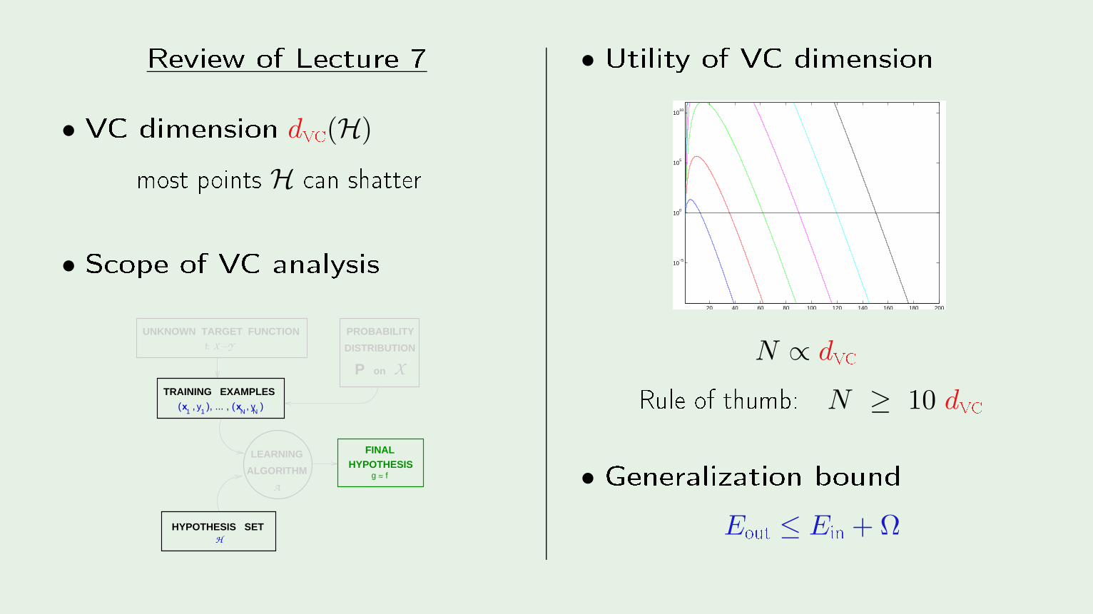
Review of Le ture 7• VC dimension dv (H)most points H an shatter• S ope of VC analysis

HYPOTHESIS SET

ALGORITHM

LEARNING FINALHYPOTHESIS

H

A

g ~ f ~

f: X Y

TRAINING EXAMPLES

UNKNOWN TARGET FUNCTION

DISTRIBUTION

PROBABILITY

onP X

x y x yNN11

( , ), ... , ( , )

up

down

• Utility of VC dimension

20 40 60 80 100 120 140 160 180 200

10−5

100

105

1010

N ∝ dv Rule of thumb: N ≥ 10 dv • Generalization bound

Eout ≤ Ein + Ω

Learning From DataYaser S. Abu-MostafaCalifornia Institute of Te hnologyLe ture 8: Bias-Varian e Tradeo

Sponsored by Calte h's Provost O e, E&AS Division, and IST • Thursday, April 26, 2012

Outline• Bias and Varian e• Learning Curves

© AML Creator: Yaser Abu-Mostafa - LFD Le ture 8 2/22

Approximation-generalization tradeoSmall Eout: good approximation of f out of sample.More omplex H =⇒ better han e of approximating f

Less omplex H =⇒ better han e of generalizing out of sampleIdeal H = f winning lottery ti ket

© AML Creator: Yaser Abu-Mostafa - LFD Le ture 8 3/22

Quantifying the tradeoVC analysis was one approa h: Eout ≤ Ein + Ω

Bias-varian e analysis is another: de omposing Eout into1. How well H an approximate f

2. How well we an zoom in on a good h ∈ H

Applies to real-valued targets and uses squared error © AM

L Creator: Yaser Abu-Mostafa - LFD Le ture 8 4/22

Start with EoutEout(g(D))= Ex

[(g(D)(x) − f(x)

)2]

ED

[Eout(g(D))

]= ED

[

Ex

[(g(D)(x) − f(x)

)2]]

= Ex

[

ED

[(g(D)(x) − f(x)

)2]]

Now, let us fo us on:ED

[(g(D)(x) − f(x)

)2]

© AML Creator: Yaser Abu-Mostafa - LFD Le ture 8 5/22

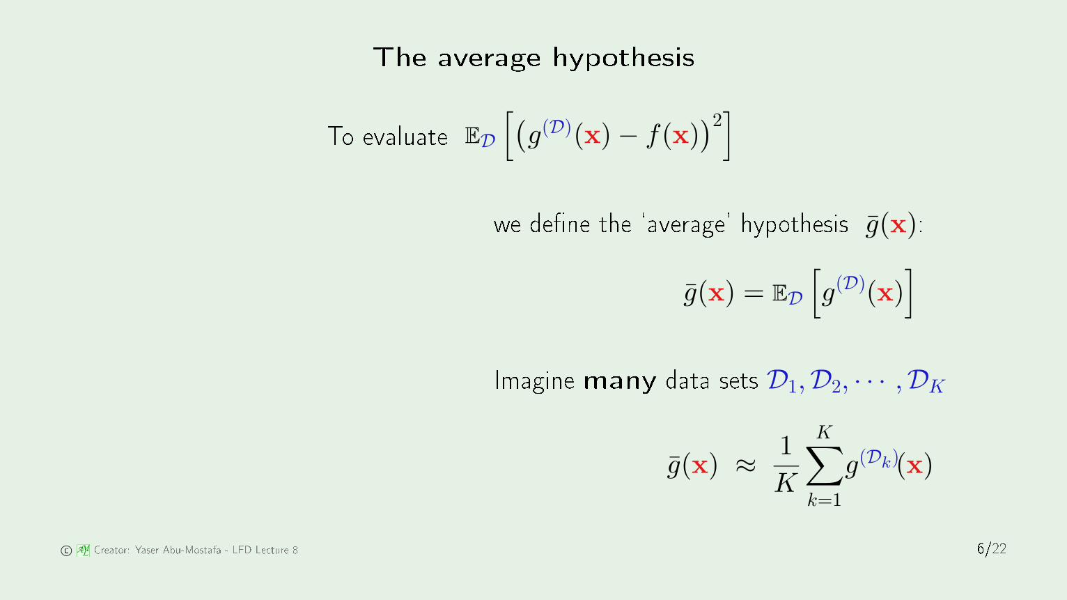
The average hypothesisTo evaluate ED

[(g(D)(x) − f(x)

)2]

we dene the `average' hypothesis g(x):g(x) = ED

[

g(D)(x)]

Imagine many data sets D1,D2, · · · ,DK

g(x) ≈1

K

K∑

k=1

g(Dk)(x)

© AML Creator: Yaser Abu-Mostafa - LFD Le ture 8 6/22

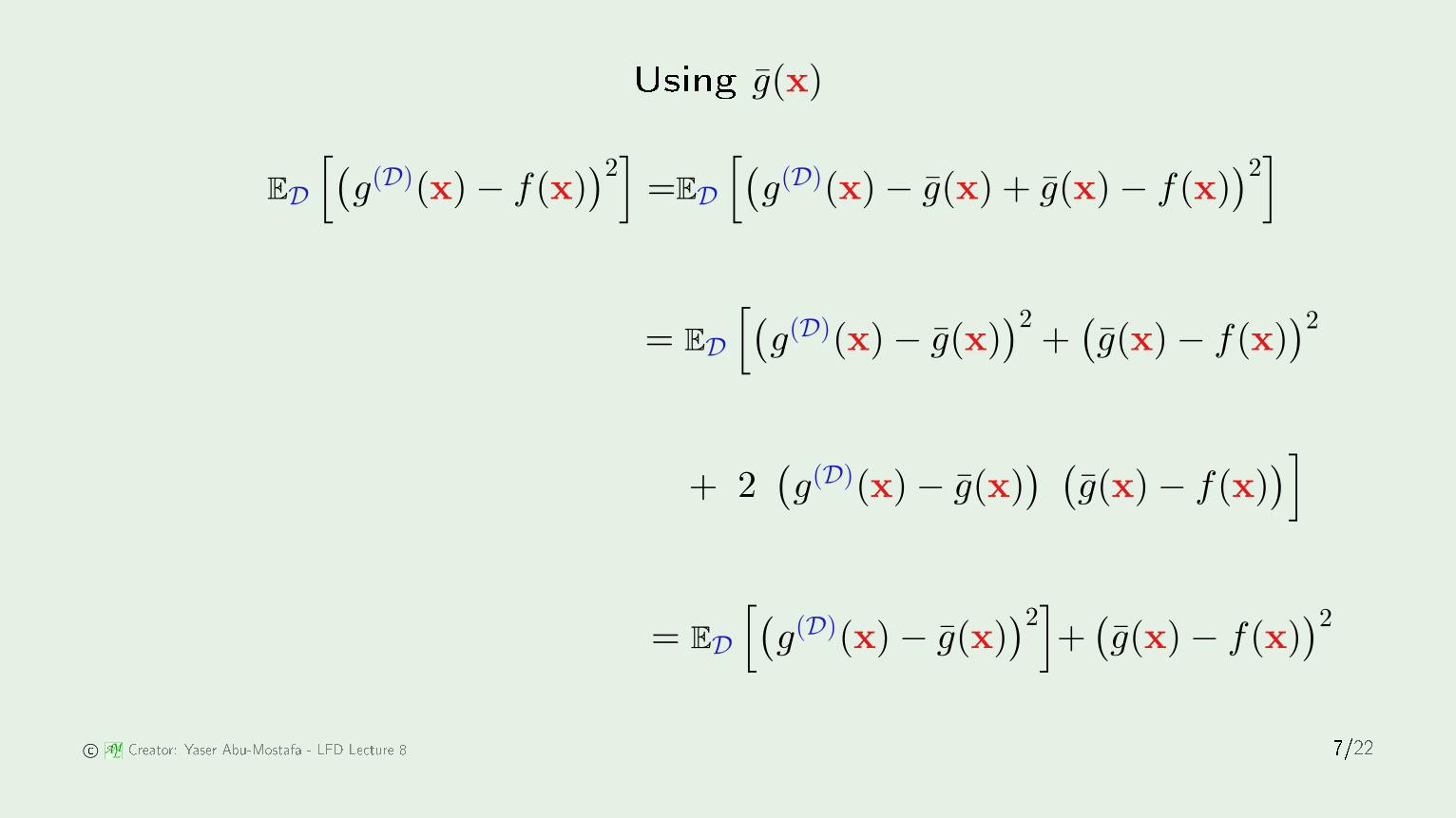
Using g(x)

ED

[(g(D)(x) − f(x)

)2]

=ED

[(g(D)(x) − g(x) + g(x) − f(x)

)2]

= ED

[(g(D)(x) − g(x)

)2+

(g(x) − f(x)

)2

+ 2(g(D)(x) − g(x)

) (g(x) − f(x)

)]

= ED

[(g(D)(x) − g(x)

)2]

+(g(x) − f(x)

)2

© AML Creator: Yaser Abu-Mostafa - LFD Le ture 8 7/22

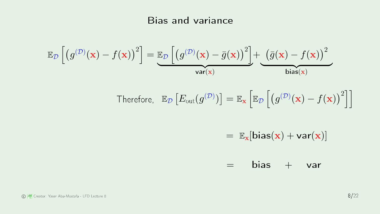
Bias and varian eED

[(g(D)(x) − f(x)

)2]

= ED

[(g(D)(x) − g(x)

)2]

︸ ︷︷ ︸var(x)

+[(

g(x) − f(x))2

]

︸ ︷︷ ︸bias(x)

Therefore, ED

[Eout(g(D))

]= Ex

[

ED

[(g(D)(x) − f(x)

)2]]

= Ex[bias(x) + var(x)]

= bias + var © AM

L Creator: Yaser Abu-Mostafa - LFD Le ture 8 8/22

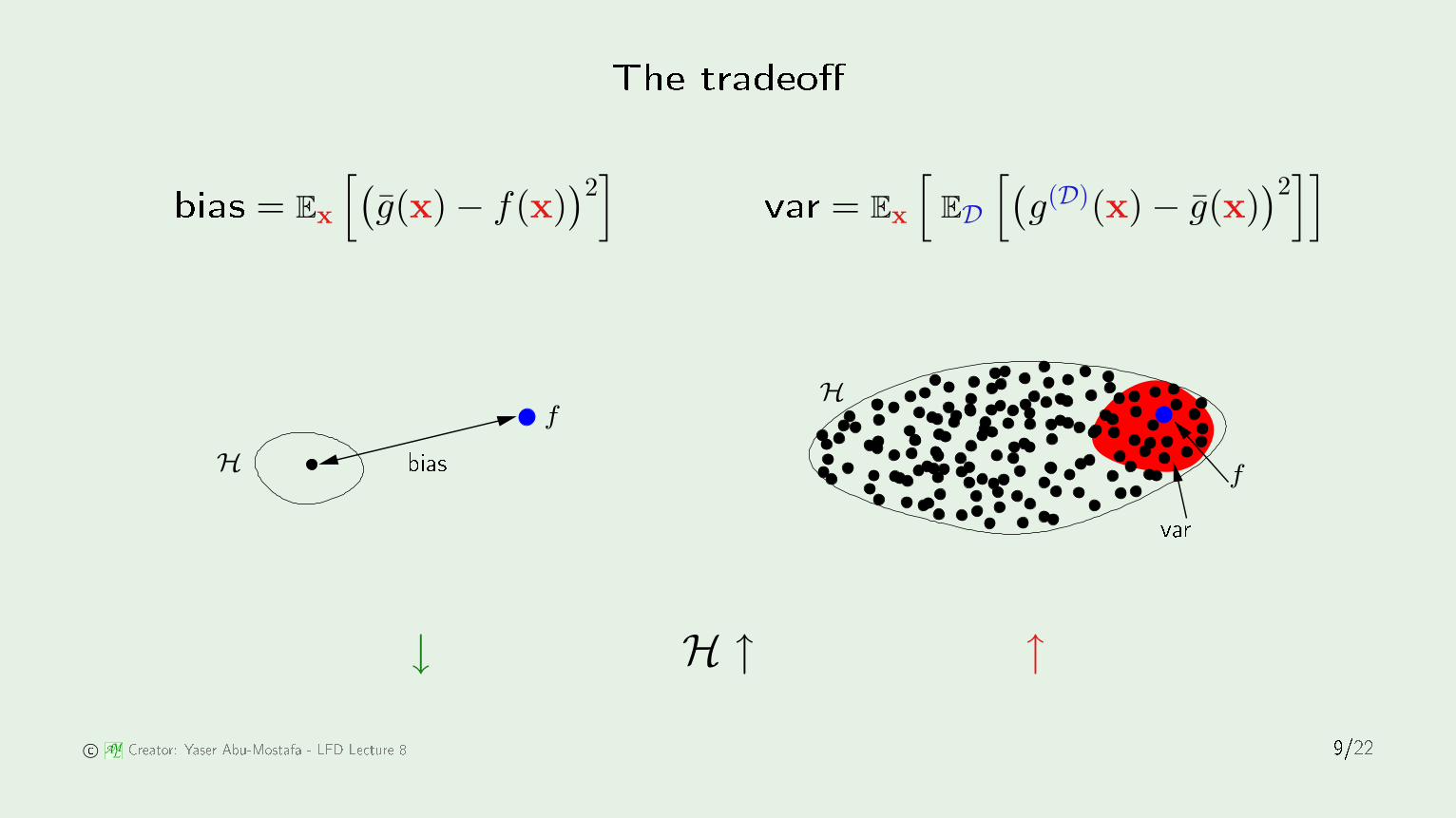
The tradeobias = Ex

[(g(x) − f(x)

)2] var = Ex

[

ED

[(g(D)(x) − g(x)

)2]]

f

H bias var f

H

↓ H ↑ ↑

© AML Creator: Yaser Abu-Mostafa - LFD Le ture 8 9/22

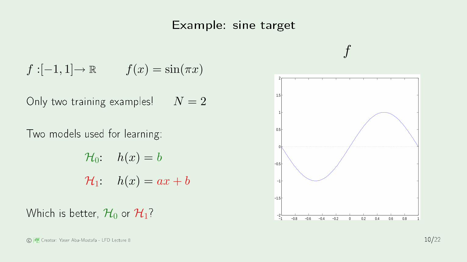
Example: sine targetH0 f

f :[−1, 1]→ R f(x) = sin(πx)

Only two training examples! N = 2

Two models used for learning:H0: h(x) = b

H1: h(x) = ax + b

Whi h is better, H0 or H1? −1 −0.8 −0.6 −0.4 −0.2 0 0.2 0.4 0.6 0.8 1−2

−1.5

−1

−0.5

0

0.5

1

1.5

2

© AML Creator: Yaser Abu-Mostafa - LFD Le ture 8 10/22

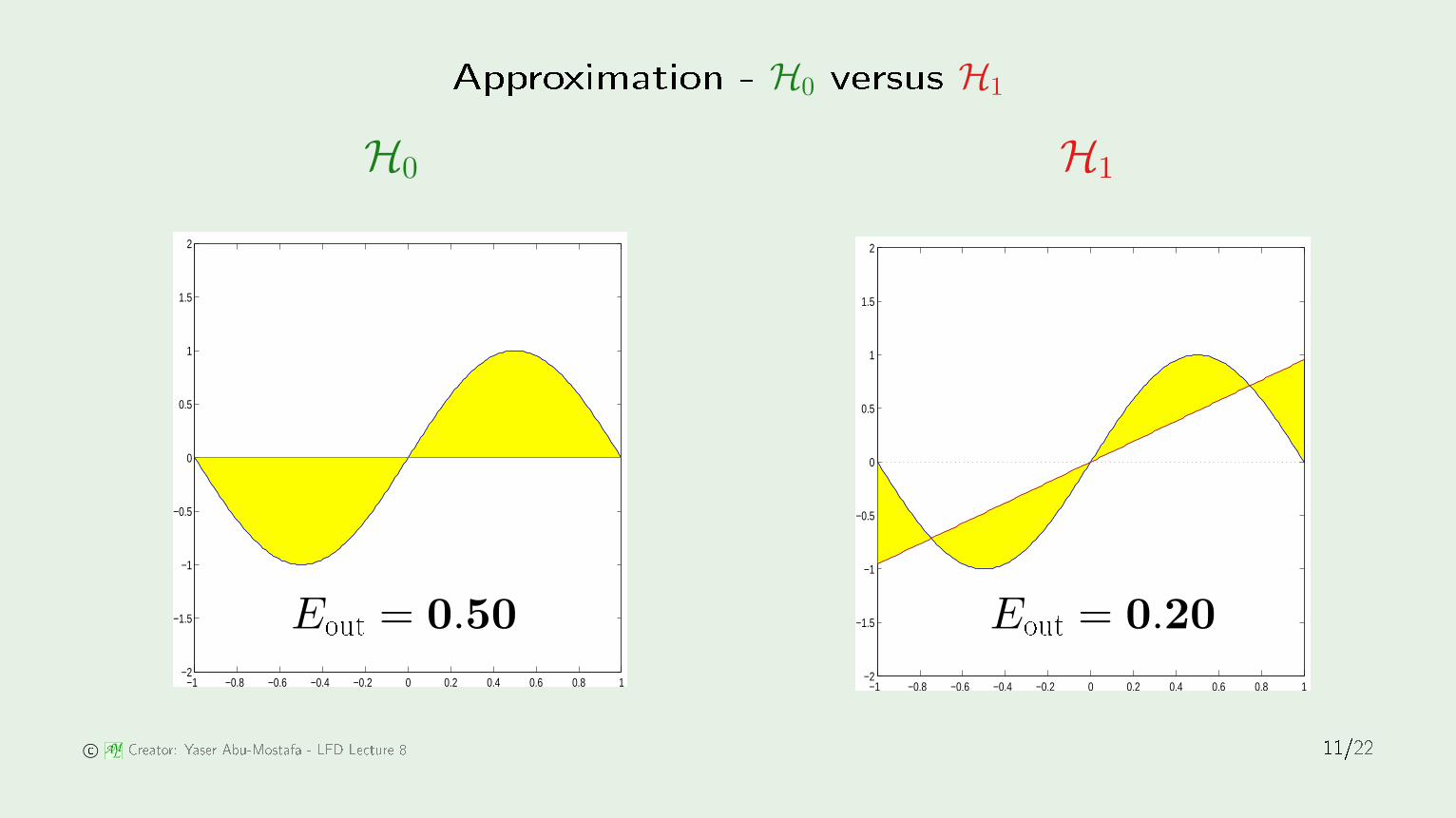
Approximation - H0 versus H1

H0 H1

−1 −0.8 −0.6 −0.4 −0.2 0 0.2 0.4 0.6 0.8 1−2

−1.5

−1

−0.5

0

0.5

1

1.5

2

−1 −0.8 −0.6 −0.4 −0.2 0 0.2 0.4 0.6 0.8 1−2

−1.5

−1

−0.5

0

0.5

1

1.5

2

Eout = 0.50 Eout = 0.20

© AML Creator: Yaser Abu-Mostafa - LFD Le ture 8 11/22

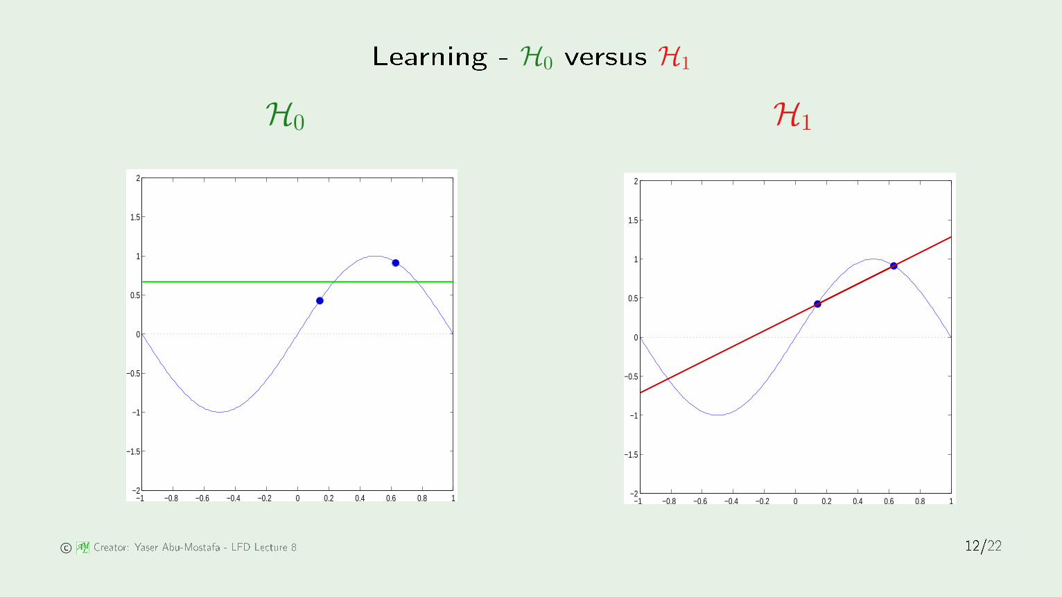
Learning - H0 versus H1

H0 H1

−1 −0.8 −0.6 −0.4 −0.2 0 0.2 0.4 0.6 0.8 1−2

−1.5

−1

−0.5

0

0.5

1

1.5

2

−1 −0.8 −0.6 −0.4 −0.2 0 0.2 0.4 0.6 0.8 1−2

−1.5

−1

−0.5

0

0.5

1

1.5

2

© AML Creator: Yaser Abu-Mostafa - LFD Le ture 8 12/22

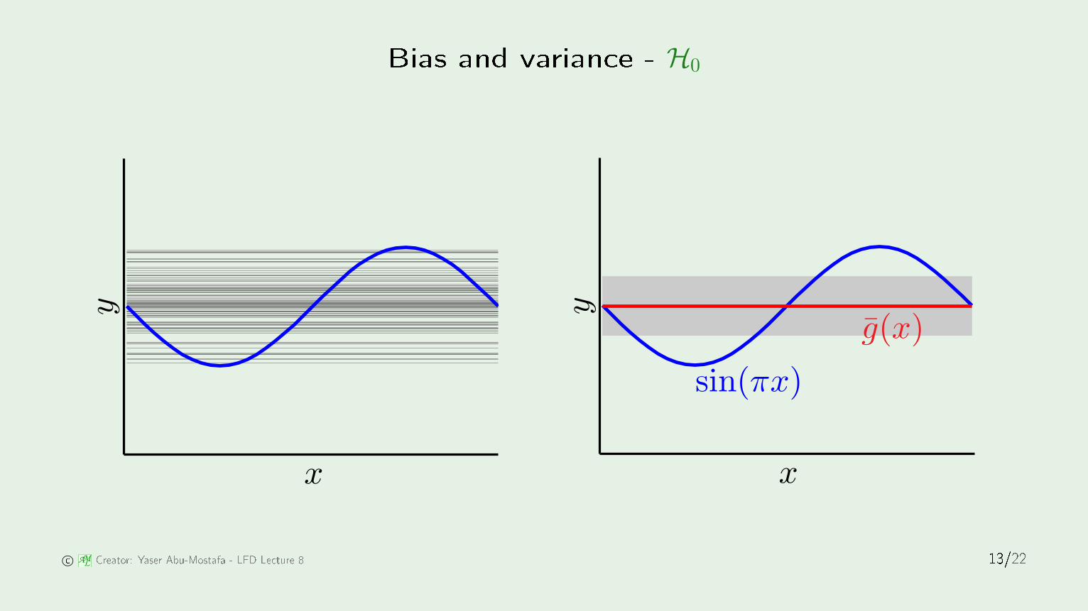
Bias and varian e - H0

PSfrag repla ements

x

y

-1-0.8-0.6-0.4-0.200.20.40.60.81-1-0.8-0.6-0.4-0.200.20.40.60.81

PSfrag repla ements

x

y

g(x)

sin(πx)

-1-0.8-0.6-0.4-0.200.20.40.60.81-1-0.8-0.6-0.4-0.200.20.40.60.81 © AM

L Creator: Yaser Abu-Mostafa - LFD Le ture 8 13/22

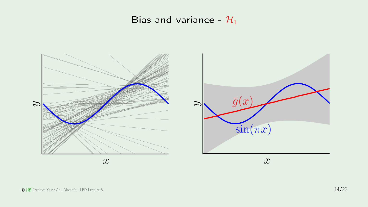
Bias and varian e - H1

PSfrag repla ements

x

y

-1-0.8-0.6-0.4-0.200.20.40.60.81-8-6-4-20246

PSfrag repla ements

x

y g(x)

sin(πx)

-1-0.8-0.6-0.4-0.200.20.40.60.81-3-2-10123 © AM

L Creator: Yaser Abu-Mostafa - LFD Le ture 8 14/22

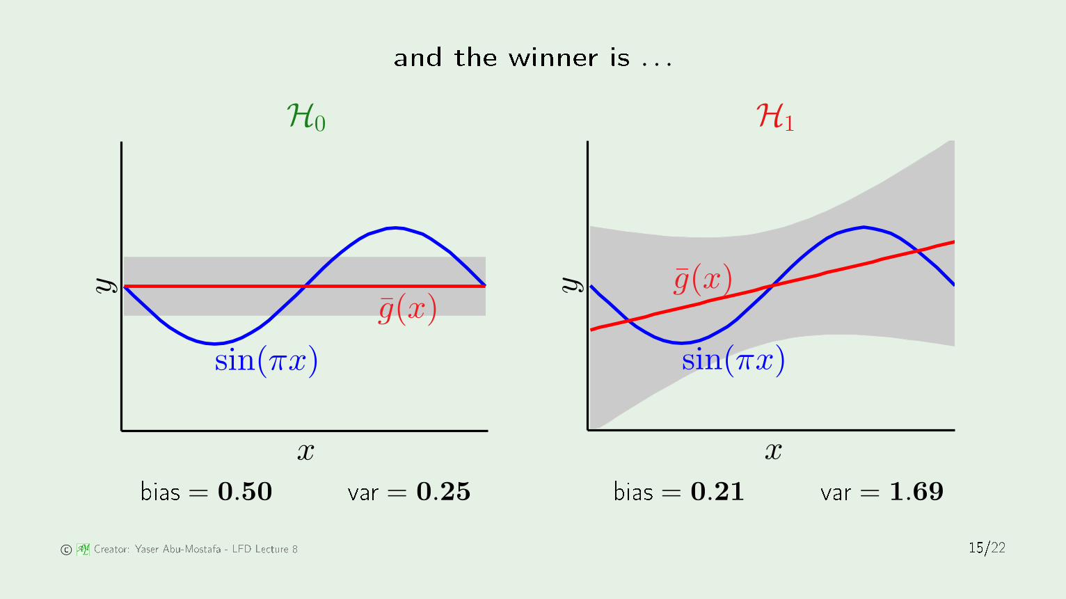
and the winner is . . .

H0 H1

PSfrag repla ements

x

y

g(x)

sin(πx)

-1-0.8-0.6-0.4-0.200.20.40.60.81-1-0.8-0.6-0.4-0.200.20.40.60.81

PSfrag repla ements

x

y g(x)

sin(πx)

-1-0.8-0.6-0.4-0.200.20.40.60.81-3-2-10123bias = 0.50 var = 0.25 bias = 0.21 var = 1.69 © AML Creator: Yaser Abu-Mostafa - LFD Le ture 8 15/22

Lesson learnedMat h the `model omplexity'

to the data resour es, not to the target omplexity

© AML Creator: Yaser Abu-Mostafa - LFD Le ture 8 16/22

Outline• Bias and Varian e• Learning Curves

© AML Creator: Yaser Abu-Mostafa - LFD Le ture 8 17/22

Expe ted Eout and EinData set D of size N

Expe ted out-of-sample error ED[Eout(g(D))]

Expe ted in-sample error ED[Ein(g(D))]

How do they vary with N?

© AML Creator: Yaser Abu-Mostafa - LFD Le ture 8 18/22

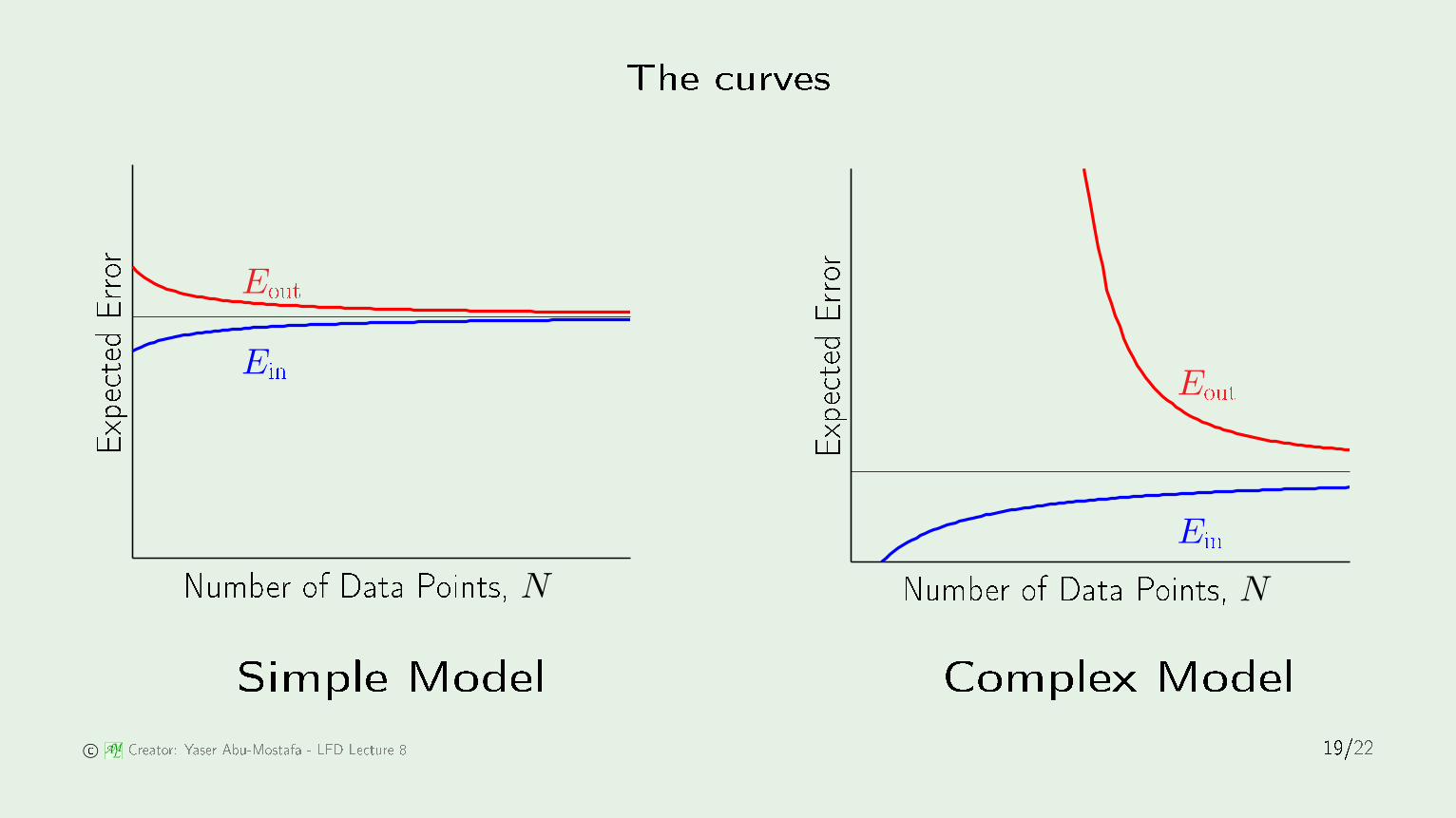
The urves

PSfrag repla ements

Number of Data Points, N

Expe tedError Eout

Ein

204060801001200.160.180.20.22

PSfrag repla ements

Number of Data Points, N

Expe tedError

EoutEin

204060801001200.050.10.150.20.25Simple Model Complex Model © AM

L Creator: Yaser Abu-Mostafa - LFD Le ture 8 19/22

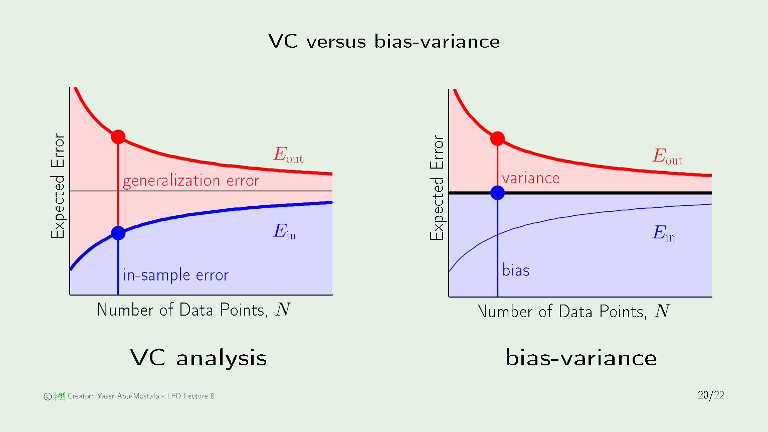
VC versus bias-varian e

PSfrag repla ements

Number of Data Points, N

Expe tedError

in-sample errorgeneralization error Eout

Ein

204060800.160.170.180.190.20.210.22

PSfrag repla ements

Number of Data Points, N

Expe tedError

biasvarian e Eout

Ein

204060800.160.170.180.190.20.210.22VC analysis bias-varian e © AM

L Creator: Yaser Abu-Mostafa - LFD Le ture 8 20/22

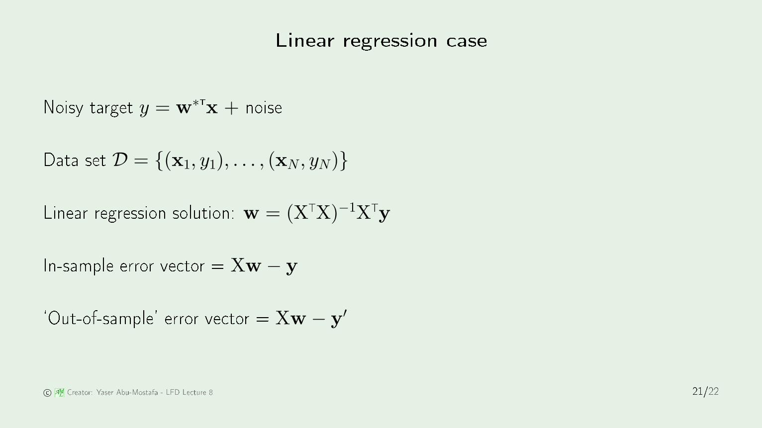
Linear regression aseNoisy target y = w∗Tx + noiseData set D = (x1, y1), . . . , (xN , yN)

Linear regression solution: w = (XTX)−1XTyIn-sample error ve tor = Xw − y

`Out-of-sample' error ve tor = Xw − y′

© AML Creator: Yaser Abu-Mostafa - LFD Le ture 8 21/22

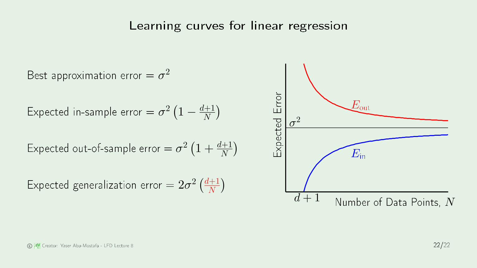
Learning urves for linear regression

PSfrag repla ements

Number of Data Points, N

Expe tedError Eout

Einσ2

d + 1

02040608010000.20.40.60.811.21.41.61.82

Best approximation error = σ2

Expe ted in-sample error = σ2(1 − d+1

N

)

Expe ted out-of-sample error = σ2(1 + d+1

N

)

Expe ted generalization error = 2σ2(

d+1N

)

© AML Creator: Yaser Abu-Mostafa - LFD Le ture 8 22/22