Embed Size (px)
Citation preview
UNIVERSITY OF UDINE - ITALY
Department of Mathematics and Computer Science
Ph.D. Thesis
DAG SCHEDULING FOR GRID
COMPUTING SYSTEMS
Supervisors: Candidate:Prof. ALESSANDRO DE ANGELIS ALBERTO FORTI
Doctorate of Philosophy in Computer Science
XVIII cycle
AY 2005/2006

Abstract
Today’s parallel and distributed systems are changing in their organization and theconcept of Grid computing, a set of dynamic and heterogeneous resources connectedvia Internet and shared by many and different users, is nowadays becoming a reality.A large number of scheduling heuristics for parallel applications described by directedacyclic graphs (DAGs) have been presented in the literature, but most of them assumea homogeneous system with a homogeneous network, i.e. a message is transmittedwith the same speed on all the links. In a Grid environment this assumption cannot bedone. In this thesis we tackle the problem of scheduling parallel applications describedby directed acyclic graphs (DAGs) in a Grid computing system.

Contents
Introduction v
1 Introduction to Grid 11.1 What is Grid . . . . . . . . . . . . . . . . . . . . . . . . . . . . . . . . 1
1.1.1 Grid challenges . . . . . . . . . . . . . . . . . . . . . . . . . . . 31.2 Grid Applications . . . . . . . . . . . . . . . . . . . . . . . . . . . . . . 4
1.2.1 Case study: the MAGIC telescope . . . . . . . . . . . . . . . . 41.3 Summary . . . . . . . . . . . . . . . . . . . . . . . . . . . . . . . . . . 7
2 Grid technologies 112.1 Brief overview of distributed systems . . . . . . . . . . . . . . . . . . . 11
2.1.1 Properties of a distributed system . . . . . . . . . . . . . . . . 122.2 The client-server model . . . . . . . . . . . . . . . . . . . . . . . . . . 132.3 Communication . . . . . . . . . . . . . . . . . . . . . . . . . . . . . . . 14
2.3.1 Remote procedure call . . . . . . . . . . . . . . . . . . . . . . . 142.3.2 Remote object invocation . . . . . . . . . . . . . . . . . . . . . 152.3.3 Message-oriented communication . . . . . . . . . . . . . . . . . 162.3.4 Stream-oriented communication . . . . . . . . . . . . . . . . . . 16
2.4 Service Oriented Architecture . . . . . . . . . . . . . . . . . . . . . . . 172.4.1 Basic components of SOA . . . . . . . . . . . . . . . . . . . . . 182.4.2 Web services as an implementation of the SOA . . . . . . . . . 19
2.5 The evolution of the Grid . . . . . . . . . . . . . . . . . . . . . . . . . 212.6 The Globus Toolkit . . . . . . . . . . . . . . . . . . . . . . . . . . . . . 222.7 Open Grid Service Architecture (OGSA) . . . . . . . . . . . . . . . . . 242.8 Web Services Resource Framework . . . . . . . . . . . . . . . . . . . . 272.9 Summary . . . . . . . . . . . . . . . . . . . . . . . . . . . . . . . . . . 29
3 Grid scheduling 313.1 Grid Resource Management Systems . . . . . . . . . . . . . . . . . . . 313.2 Introduction to Grid scheduling . . . . . . . . . . . . . . . . . . . . . . 33
3.2.1 General Architecture of a Grid Scheduler . . . . . . . . . . . . 353.3 Grid Workflows . . . . . . . . . . . . . . . . . . . . . . . . . . . . . . . 363.4 Grid scheduling systems . . . . . . . . . . . . . . . . . . . . . . . . . . 39
3.4.1 Condor DAGMan . . . . . . . . . . . . . . . . . . . . . . . . . . 393.4.2 GrADS . . . . . . . . . . . . . . . . . . . . . . . . . . . . . . . 403.4.3 UNICORE . . . . . . . . . . . . . . . . . . . . . . . . . . . . . 41
3.5 Summary . . . . . . . . . . . . . . . . . . . . . . . . . . . . . . . . . . 41
ii Contents
4 Literature survey of the DAG scheduling problem 434.1 The DAG scheduling problem . . . . . . . . . . . . . . . . . . . . . . . 43
4.1.1 NP-completeness of the DAG scheduling problem . . . . . . . . 464.2 Background . . . . . . . . . . . . . . . . . . . . . . . . . . . . . . . . . 47
4.2.1 The computing system . . . . . . . . . . . . . . . . . . . . . . . 484.2.2 DAG scheduling preliminaries . . . . . . . . . . . . . . . . . . . 484.2.3 Clustering of a DAG: communication and granularity . . . . . 52
4.3 Scheduling of Primitive Graph Structures . . . . . . . . . . . . . . . . 554.4 Taxonomy of DAG scheduling algorithms . . . . . . . . . . . . . . . . 564.5 Properties of list scheduling . . . . . . . . . . . . . . . . . . . . . . . . 584.6 DAG scheduling algorithms . . . . . . . . . . . . . . . . . . . . . . . . 59
4.6.1 Polynomial-time algorithm for Tree-Structured DAGs . . . . . 604.6.2 Arbitrary graphs for a two-processor system . . . . . . . . . . . 604.6.3 Scheduling of Interval-Ordered DAGs . . . . . . . . . . . . . . 614.6.4 Sarkar’s algorithm . . . . . . . . . . . . . . . . . . . . . . . . . 624.6.5 The HLFET algorithm . . . . . . . . . . . . . . . . . . . . . . . 624.6.6 The ETF algorithm . . . . . . . . . . . . . . . . . . . . . . . . 624.6.7 The ISH algorithm . . . . . . . . . . . . . . . . . . . . . . . . . 634.6.8 The FLB algorithm . . . . . . . . . . . . . . . . . . . . . . . . 634.6.9 The DSC algorithm . . . . . . . . . . . . . . . . . . . . . . . . 634.6.10 The CASS-II algorithm . . . . . . . . . . . . . . . . . . . . . . 644.6.11 The DCP algorithm . . . . . . . . . . . . . . . . . . . . . . . . 654.6.12 The MCP algorithm . . . . . . . . . . . . . . . . . . . . . . . . 664.6.13 The MD algorithm . . . . . . . . . . . . . . . . . . . . . . . . . 664.6.14 The Hybrid Remapper algorithm . . . . . . . . . . . . . . . . . 66
4.7 Summary . . . . . . . . . . . . . . . . . . . . . . . . . . . . . . . . . . 68
5 A DAG scheduling algorithm for Grid computing systems 715.1 The computing system environment . . . . . . . . . . . . . . . . . . . 715.2 Considerations on the design of the algorithm . . . . . . . . . . . . . . 735.3 Preliminaries . . . . . . . . . . . . . . . . . . . . . . . . . . . . . . . . 745.4 The CCF algorithm . . . . . . . . . . . . . . . . . . . . . . . . . . . . 74
5.4.1 Considerations . . . . . . . . . . . . . . . . . . . . . . . . . . . 745.4.2 Assumptions . . . . . . . . . . . . . . . . . . . . . . . . . . . . 755.4.3 First version of the algorithm . . . . . . . . . . . . . . . . . . . 765.4.4 Analysis of the algorithm . . . . . . . . . . . . . . . . . . . . . 795.4.5 Final version of the algorithm . . . . . . . . . . . . . . . . . . . 845.4.6 Join DAG analysis for the final version of the algorithm . . . . 85
5.5 A variant of the DSC algorithm . . . . . . . . . . . . . . . . . . . . . . 875.6 Summary . . . . . . . . . . . . . . . . . . . . . . . . . . . . . . . . . . 88
Contents iii
6 Experimental Results 896.1 Simulation framework . . . . . . . . . . . . . . . . . . . . . . . . . . . 89
6.1.1 The simulator . . . . . . . . . . . . . . . . . . . . . . . . . . . . 906.1.2 DAG generation . . . . . . . . . . . . . . . . . . . . . . . . . . 906.1.3 Platform generation . . . . . . . . . . . . . . . . . . . . . . . . 91
6.2 Performance comparisons . . . . . . . . . . . . . . . . . . . . . . . . . 926.3 Summary . . . . . . . . . . . . . . . . . . . . . . . . . . . . . . . . . . 96
Conclusions 99
Bibliography 101

iv Contents

Introduction
The subject of this thesis is the scheduling of parallel applications described by di-rected acyclic graphs (DAGs) in Grid computing systems. Basically, Grid is a geo-graphical distributed system. Distributed computing scaled to a global level with thematuration of the Internet in the 1990s. Advances in networking technologies willsoon make it possible to use the global information infrastructure in a qualitativelydifferent way, as a computational as well as an information resource. The last decadehas seen a substantial increase in commodity computer and network performance, asa result of faster hardware, low costs and more sophisticated software. Nevertheless,there are problems in the fields of science, engineering, and business, which cannot beeffectively dealt with using the current generation of supercomputers. Usually theseproblems are computational and data intensive and consequently need heterogeneousresources not available in a single organization. The ubiquity of the Internet andthe availability of high-speed networks leads to the possibility of using wide-area dis-tributed computers for solving large-scale problems. Such an approach to networkcomputing is known by several names: metacomputing, scalable computing, globalcomputing, Internet computing, Peer-to-Peer (P2P) and Grid computing.
Grids enable the sharing, selection, and aggregation of a wide variety of resourcesincluding supercomputers, storage systems, data sources, and specialized devices thatare geographically distributed and owned by different organizations. The Grid allowsusers to solve larger-scale problems by pooling together resources that could not becoupled easily before.
The concept of Grid computing started as a project to link geographically dis-persed supercomputers, but now it has grown far beyond its original intent. Dueto the rapid growth of the Internet and Web, there has been a growing interest inWeb-based distributed computing, and many projects have been started and aim toexploit the Web as an infrastructure for running coarse-grained distributed and par-allel applications. In fact, like any other growing idea, the Grid has evolved passingthrough different phases. Nowadays we are in the third Grid generation [106]. Thisgeneration defines the Grid as a service oriented architecture based on web services.In this context, the Web has the capability to act as a platform for parallel andcollaborative work as well as a key technology to create a pervasive and ubiquitousGrid-based infrastructure.
The design of Grid as a service oriented architecture have led to a growing interestin workflows by the Grid community. The reason is that the “software as a service”approach results in a componentized view of software applications and workflow cannaturally be used as a component composition mechanism. Traditionally, the mainapplications of workflows have been in the automation of administrative and produc-tion processes, especially within businesses and large organizations. The expansion
vi Introduction
of workflow towards middleware is realized within the Web service initiative. Gridworkflows are an emerging research field in the Grid community and there is an ongo-ing effort to define a standard meaning of workflow for the Grid. Actually, the mostcommon Grid workflow can be modelled as simple Task (Directed Acyclic) Graphs(DAGs), where the order of execution of tasks (modelled as nodes) is determined bydependencies (in turn modelled as directed arcs). Each DAG node represents theexecution of a component, characterized by a set of attributes such as an estimateof its cost and possible requirements on the target execution platform, while DAGdirected edges represent data dependencies between specific application components.Data dependencies will be usually constituted by large files written by a componentand required for the execution of one or more other components of the application.Two types of DAGs can be distinguished: coarse grained DAGs, in which the compu-tation is dominant with respect to communication, and fine grained DAGs, in whichthe communication is dominant with respect to computation.
One of the most active areas of research in the Grid community is scheduling.Scheduling in Grid means taking decisions involving resources distributed over mul-tiple administrative domains. The main difference between a Grid scheduler and alocal scheduler is that the former does not own the resources at a local site and hasno control over them. In particular it doesn’t know if other users are sending jobsto the resources that it is considering. Grid is a dynamic environment and resourcescome and go, therefore a scheduler has to be able to discover and monitor the re-sources. In general, Grid schedulers get information from a general Grid InformationSystem (GIS) that in turn gathers information from individual local resources. TheGlobus Monitoring and Discovery Service [26] is an example of Grid service thatallows the monitoring and the discovery of the resources. Another example is theNetwork Weather System [130] that is a distributed monitoring system designed totrack and forecast dynamic resource conditions, e.g. it allows a user or a program(such as a scheduler) to request information (latency, bandwidth, load, estimates, etc)for entities corresponding to network links connecting specified endpoints, retrieve thefraction of CPU available to a newly started process, retrieve the amount of memorythat is currently unused in a remote host, etc.
The problem of scheduling DAGs in a heterogeneous environment is NP-complete.To tackle the problem, simplifying assumptions have been made regarding the taskgraph structure representing the program and the model for the parallel processorsystem. However, it is NP-complete even in two simple cases: (1) scheduling unit-timetasks to an arbitrary number of processors [58], (2) scheduling one or two time unittasks to two processors [22]. Many DAG scheduling algorithms can be found in theliterature. Usually they do not impose constraints on the graph structure but many ofthem assume a homogeneous computing system. The reason is that they were designedto schedule parallel applications in clusters. For the same reason the algorithmsthat consider heterogeneous systems assume a homogeneous interconnection network,i.e. all the links have the same latency and bandwidth and, therefore, messages aretransmitted with the same speed on all the links. Very few works do not impose anyconstraint on the networked computing system.
The DAG scheduling problem is usually identified by the combination of two
Introduction vii
phases: matching which assigns tasks to machines and scheduling which defines theexecution order of the tasks assigned to each machine. The overall problem of match-ing and scheduling is referred to as mapping.
Due to the intractability of the general scheduling problem, many heuristics havebeen suggested to tackle it under more generic situations. A heuristic produces ananswer in less than exponential time but does not guarantee an optimal solution. Themost popular approach to the design of scheduling algorithms is the list schedulingtechnique. Tasks are associated to priorities and a selection phase chooses the onewith higher priority. The selected task is then mapped to an appropriate resource.In order to find a good schedule, the scheduler must take care of these two aspects:
• Map a task to a resource that allows to complete the execution of that task assoon as possible.
• Minimize data transfer times.
Obviously it is impossible to optimize both aspects at the same time, a tradeoff mustbe found. In particular, minimization of the data transfer times can be accomplishedin two ways: by mapping the communicating tasks onto two resources close to eachother or with the zeroing of the communication time by mapping the two tasks ontothe same resource. Usually, the tradeoff point is between parallelization and sequen-tialization. To sequentialize means mapping parallel tasks onto the same resource,sequentialization allows to zero incoming or outgoing edges connecting the two tasksto a common parent or child. What emerges from the literature is that algorithmsbased on Critical Path (CP) heuristics are the ones giving, on average, the best resultsin terms of quality of the schedule produced, i.e. reduction of the completion time ofthe entire workflow. The CP is the weight of the longest path of the DAG and pro-vides an upper bound on the schedule length. In order to keep track of the CP duringthe scheduling some algorithms consider nodes belonging to the Dominant Sequence(DS), that is the CP of the scheduled DAG. Anyway, even these dynamic heuristicscan get trapped in a locally optimal decision, leading to a non-optimal global solution.This means that scheduling at each step a DS node may not be the correct choice.
This thesis aims at studying algorithms for scheduling DAGs in a Grid computingsystem. We first have analyzed the problem of scheduling in the Grid and then wehave studied how the DAG scheduling algorithms found in the literature work. Thefinal goal of this thesis is to propose a novel scheduling algorithm to address theproblem of scheduling DAG described parallel applications in Grid. A modification ofthe well known DSC [135] algorithm is also presented. We have conducted extensivesimulation tests in order to compare the results of the two proposed algorithms withother reference algorithms.
Thesis outline
This thesis is divided into six chapters, which are organized as follows.
viii Introduction
In order to make the reader familiar with Grid computing, in chapter 1 we presentan introduction to Grid, together with a case study of the migration to Grid of theastroparticle experiment (in which we have participated) MAGIC.
In chapter 2 we describe the evolution of Grid together with the technologies thatenables this new paradigm of computation.
In chapter 3 we review Grid scheduling issues and challenges. Then, we considerhow workflows have been characterized by the Grid community and we review someGrid scheduling systems developed in the last years.
In chapter 4 we explain in detail the DAG scheduling problem and review theactual state of the art of scheduling algorithms.
In chapter 5 we propose two DAG scheduling algorithms designed to work in Grid.The first one is called CCF (Cluster ready Children First) and the second one, theDSC VAR, is a variant of the famous DSC. Some properties of the proposed CCFalgorithm are identified and analyzed.
Finally, chapter 6 presents experimental results obtained with the simulation ofthe proposed algorithms CCF and DSC VAR.
1Introduction to Grid
Next generation scientific exploration requires computing power and storage that nosingle institution alone is able to afford. Additionally, easy access to distributed datais required to improve the sharing of results by scientific communities spread aroundthe world. The proposed solution to these challenges is to enable different institu-tions, working in the same scientific field, to put their computing, storage and dataresources together in order to achieve the required performance and scale. Grid isa type of parallel and distributed system that enables the sharing, selection, andaggregation of services of heterogeneous resources distributed across “multiple” ad-ministrative domains based on their availability, capability, performance, cost, andusers’ quality-of-service requirements. As Network performance has outpaced com-putational power and storage capacity, this new paradigm has evolved to enable thesharing and coordinated use of geographically distributed resources. This chapterpresents an introduction to Grid giving focus to the main requirements and challengesthat must be addressed in setting up this new paradigm of distributed computing.
1.1 What is Grid
The ancestor of the Grid is Metacomputing. This term was coined in the earlyeighties. The idea of Metacomputing was to interconnect a collection of computersheld together by state-of-the-art technology and ”balanced” so that, to the individualuser, it looks and acts like a single computer. The constituent parts of the resulting“metacomputer” could be housed locally, or distributed between buildings, even con-tinents. One of the first infrastructures in this area, named Information Wide AreaYear (I-WAY) [41], was demonstrated at Supercomputing 1995. This project stronglyinfluenced the subsequent Grid computing activities. In fact one of the researcherswho lead the project I-WAY was Ian Foster who along with Carl Kesselman publishedin 1997 a paper [42] that clearly links the Globus Toolkit, which is currently the heartof many Grid projects, to Metacomputing.
Foster and Kesselman published in 1998 the book “The Grid: Blueprint for a NewComputing Infrastructure”[43], which is considered the “Grid bible”. They definedthe Grid as follows: A computational Grid is a hardware and software infrastructurethat provides dependable, consistent, pervasive, and inexpensive access to high-end
2 1. Introduction to Grid
computational capabilities. In fact one of the main ideas of the Grid, which alsoexplains the origin of the word itself, was to make computational resources availablelike electricity. One remarkable fact of the electric power grid infrastructure is thatwhen we plug an appliance into it we do not care where the generators are locatedand how they are wired. We are only interested in getting the electric power, andthat’s all! Unfortunately, in practice, the similarities between the electric power gridand the computational Grid are very few.
According to a Foster’s check list the minimum properties of a Grid system arethe following [47]:
• A Grid coordinates resources that are not subject to centralized control (e.g.resources owned by different companies or under the control of different admin-istrative units) and at the same time addresses the issues of security, policy,payment, membership, and so forth that arise in these settings.
• A Grid must use standard, open, general-purpose protocols and interfaces.These protocols address fundamental issues such as authentication, authoriza-tion, resource discovery, and resource access.
• A Grid delivers nontrivial quality service, i.e. it is able to meet complex userdemands (e.g. response time, throughput, availability, security, etc.).
This checklist gives focus to what is the key concept of Grid computing: theability to negotiate resource-sharing arrangements among a set of participating parties(providers and consumers). The “sharing” refers not only to file exchange but alsoto direct access to computers, software, data, and other resources. This sharing haveto be highly controlled with resource providers and consumers defining clearly andcarefully just what is shared, who is allowed to share, and the conditions under whichsharing occurs. A set of individuals and/or institutions defined by such sharing rulesforms a virtual organization.
Basically, the vision that is now becoming reality is as follows:
• The user submits his request through a Graphical User Interface (GUI) justspecifying high level requirements (the kind of application he wants to use, theoperating system,...) and possibly providing input data.
• The Grid finds and allocates suitable resources (computing systems, storagefacilities, etc.) to satisfy the user’s request.
• The Grid monitors request processing.
• The Grid notifies the user when the results are available allowing their retrieval.
Grid can be seen as the latest and most complete evolution of more familiardevelopments such as distributed computing, the Web, peer-to-peer computing andvirtualization technologies:
• Like the Web, Grid computing keeps complexity hidden: multiple users enjoy asingle, unified experience.
1.1. What is Grid 3
• Unlike the Web, which mainly enables communication, Grid computing enablesfull collaboration toward common business goals.
• Like peer-to-peer, Grid computing allows users to share files.
• Unlike peer-to-peer, Grid computing allows many-to-many sharing not only filesbut other resources as well.
• Like clusters and distributed computing, Grids bring computing resources to-gether.
• Unlike clusters and distributed computing, which need physical proximity andoperating homogeneity, Grids can be geographically distributed and heteroge-neous.
• Like virtualization technologies, Grid computing enables the virtualization ofIT resources.
• Unlike virtualization technologies, which virtualize a single system, Grid com-puting enables the virtualization of vast and disparate IT resources.
1.1.1 Grid challenges
There are many challenges that must be addressed in order to build a working Gridenvironment. The following list shows the main requirements a Grid should satisfy,or equivalently the main services a Grid should make available:
• Information services: Concerns information about the resources available onthe Grid. It includes the set of available resources, hardware specifications aswell dynamic information like load and forecasts. These information should beautomatically maintained and kept up to date.
• Resource brokering: Grid users should submit their requests to a resourcebroker specifying their high level requirements. The Resource Broker should beable to find and allocate suitable resources by querying information services.
• Uniform access to resources: all the resources of the same kind (computingelements, storage elements, etc.) should be accessed in a uniform way, no matterwhich technologies or standards they are based on. Middleware installed oneach single machine is a way for hiding heterogeneity and for providing uniforminterfaces.
• Security: Security mechanisms are needed in order to enable system adminis-trators to enforce access rules for all the resources made available on the Grid.This point is strongly related with the concept of virtual organization. A num-ber of issues must be addressed inside the security context [46]:
– Single sign-on. A single computation may entail access to many resources,but a user should be able to authenticate once and then assign to thecomputation the right to operate on his or her behalf.
4 1. Introduction to Grid
– Mapping to local security mechanisms. Different sites may use differentlocal security solutions. A Grid security infrastructure needs to map tothese local solutions at each site, so that local operations can proceed withappropriate privileges.
– Delegation. A computation that spans many resources creates sub-computationsthat may themselves generate requests to other resources and services,perhaps creating additional subcomputations, and so on. Authenticationoperations are involved at each stage.
– Community authorization and policy. In a large community, the policiesthat govern who can use which resources for what purpose cannot be baseddirectly on individual identity. It is infeasible for each resource to keeptrack of community membership and privileges. Instead, resources (andusers) need to be able to express policies in terms of other criteria, such asgroup membership, which can be identified with a cryptographic credentialissued by a trusted third party.
• Job scheduling: Jobs submitted by the users should be effectively and effi-ciently scheduled.
• Data Access: Grid users should be able to access distributed data in a uniformway.
• Data replication: Grids should allow automatic file replica creation in orderto move data closer to the user or to the computing facilities that will processthem. It is also a way to increase the fault-tolerance of the system.
1.2 Grid Applications
Currently there is a big effort in helping applications to migrate to Grid. An exampleis the EGEE (Enabling Grids for E-sciencE) project [34]. The project aims to pro-vide researchers in academia and industry with access to major computing resources,independently of their geographic location. The EGEE project will also focus on at-tracting a wide range of new users to the Grid. Two pilot application domains havebeen selected to guide the implementation and certify the performance and function-ality of the evolving infrastructure. One is the Large Hadron Collider ComputingGrid, supporting HEP (High Energy Physic) physics experiments, and the other isBiomedical Grids, where several communities are facing equally daunting challengesto cope with the flood of bioinformatics and healthcare data.
Just to give an example, in the following section we briefly describe the recentmigration to Grid of one astroparticle physics experiment: the MAGIC telescope.
1.2.1 Case study: the MAGIC telescope
The MAGIC (Major Atmospheric Gamma Imaging Cerenkov telescope) telescope hasbeen designed to search the sky to discover or observe high energy γ-rays sources and
1.2. Grid Applications 5
address a large number of physics questions [87]. Located at the Instituto Astro-physico de Canarias on the island La Palma, Spain, at 28◦ N and 18◦ W, at altitude2300m asl, it is the largest γ-ray telescope in the world. MAGIC is operating sinceOctober 2003, data are taken regularly since February 2004 and signals from Craband Markarian 421 was seen.
The main characteristics of the telescope are summarized below:
• A 17m diameter (f/d=1) tessellated mirror mounted on an extremely lightcarbon-fiber frame (< 10 tons), with active mirror control. The reflecting sur-face of mirrors is 240m2; reflectivity is larger than 85% (300 - 650nm).
• Elaborate computer-driven control mechanism.
• Fast slewing capability (the telescope moves 180◦ in both axes in 22s).
• A high-efficiency, high-resolution camera composed by an array of 577 fast pho-tomultipliers (PMTs), with a 3.9◦ field of view.
• Digitalization of the analogue signals performed by 300 MHz FlashADCs and ahigh data acquisition rate of up to 1 KHz.
• MAGIC is the lowest threshold (≈ 30 GeV) IACT operating in the world.
γ-ray observation in the energy range from a few tenths of GeV upwards, in overlapwith satellite observations and with substantial improvements in sensitivity, energyand angular resolution, leads to search behind the physics that has been predictedand new avenues will open. Understanding of AGNs, GRBs, SNRs, Pulsars, diffusephoton background, unidentified EGRET sources, particle physics, darkmatter, quan-tum gravity and cosmological γ-ray horizon are some of the physics goals that can beaddressed with the MAGIC telescope.
Benefits of Grid computing for MAGIC
The collaborators of the MAGIC telescope are mainly spread over Europe, 18 insti-tutions from 9 countries, with the main contributors (90% of the total) located inGermany (Max-Planck-Institute for Physics, Munich and University of Wuerzburg),Spain (Barcelona and Madrid), Italy (INFN and Universities of Padova, Udine andSiena).
The geographical distribution of the resources makes the management of the ex-periment harder. This is a typical situation for which Grid computing can be of greathelp, because it allows researchers to access all the resources in a uniform, transpar-ent and easy way. The telescope is in operation during moonless nights. The averageamount of raw FADC data recorded is about 500-600 GB/night. Additional data fromthe telescope control system or information from a weather station are also recorded.All these information have to be taken into account in the data analysis.
The MAGIC community can leverage from Grid facilities in areas like file sharing,Monte Carlo data production and analysis [40]. In a Grid scenario the system canbe accessed through a web browser based interface with single sign-on authentication
6 1. Introduction to Grid
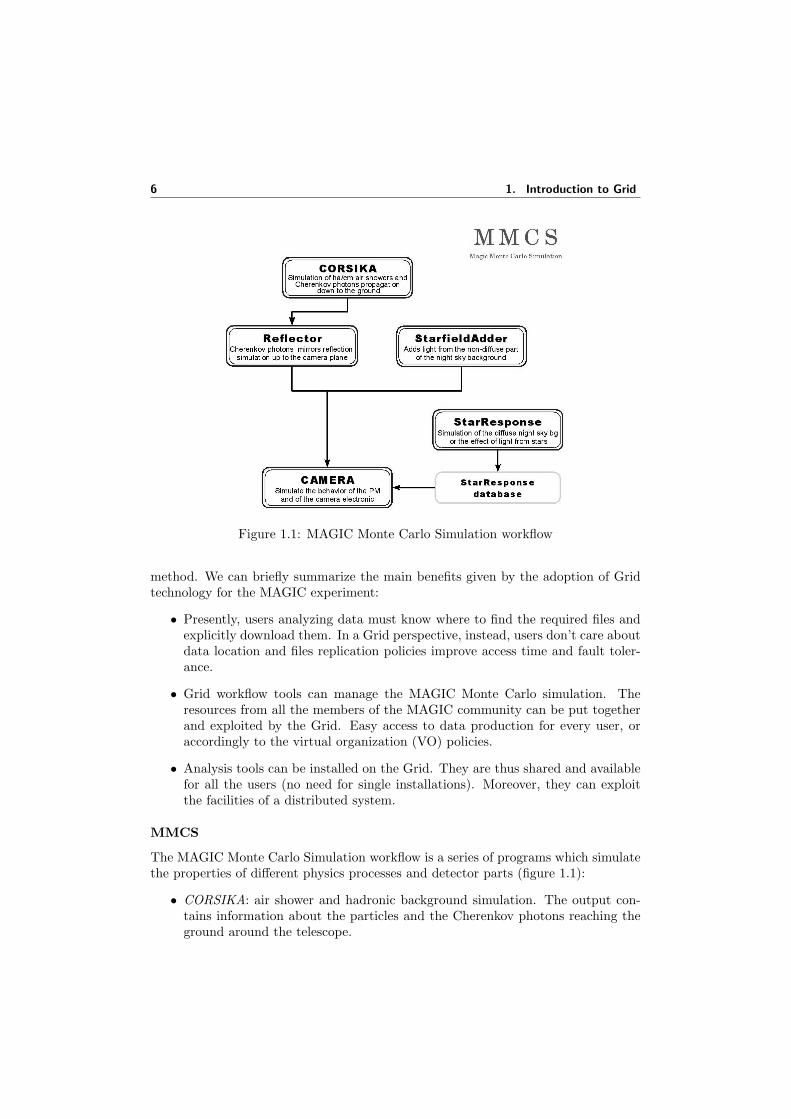
Figure 1.1: MAGIC Monte Carlo Simulation workflow
method. We can briefly summarize the main benefits given by the adoption of Gridtechnology for the MAGIC experiment:
• Presently, users analyzing data must know where to find the required files andexplicitly download them. In a Grid perspective, instead, users don’t care aboutdata location and files replication policies improve access time and fault toler-ance.
• Grid workflow tools can manage the MAGIC Monte Carlo simulation. Theresources from all the members of the MAGIC community can be put togetherand exploited by the Grid. Easy access to data production for every user, oraccordingly to the virtual organization (VO) policies.
• Analysis tools can be installed on the Grid. They are thus shared and availablefor all the users (no need for single installations). Moreover, they can exploitthe facilities of a distributed system.
MMCS
The MAGIC Monte Carlo Simulation workflow is a series of programs which simulatethe properties of different physics processes and detector parts (figure 1.1):
• CORSIKA: air shower and hadronic background simulation. The output con-tains information about the particles and the Cherenkov photons reaching theground around the telescope.
1.3. Summary 7
• Reflector : simulates the propagation of Cherenkov photons through the atmo-sphere and their reflection in the mirror up to the camera plane. The input forthe Reflector program is the output of CORSIKA.
• StarfieldAdder : simulation of the field of view. It adds light from the non-diffusepart of the night sky background, or the effect of light from stars, to imagestaken by the telescope.
• StarResponse: simulation of the night sky background (NSB) response.
• Camera: simulate the behavior of the photomultipliers and of the electronic ofthe MAGIC camera. It also allows to introduce the NSB (optionally), from thestars and/or the diffuse NSB.
Architecture
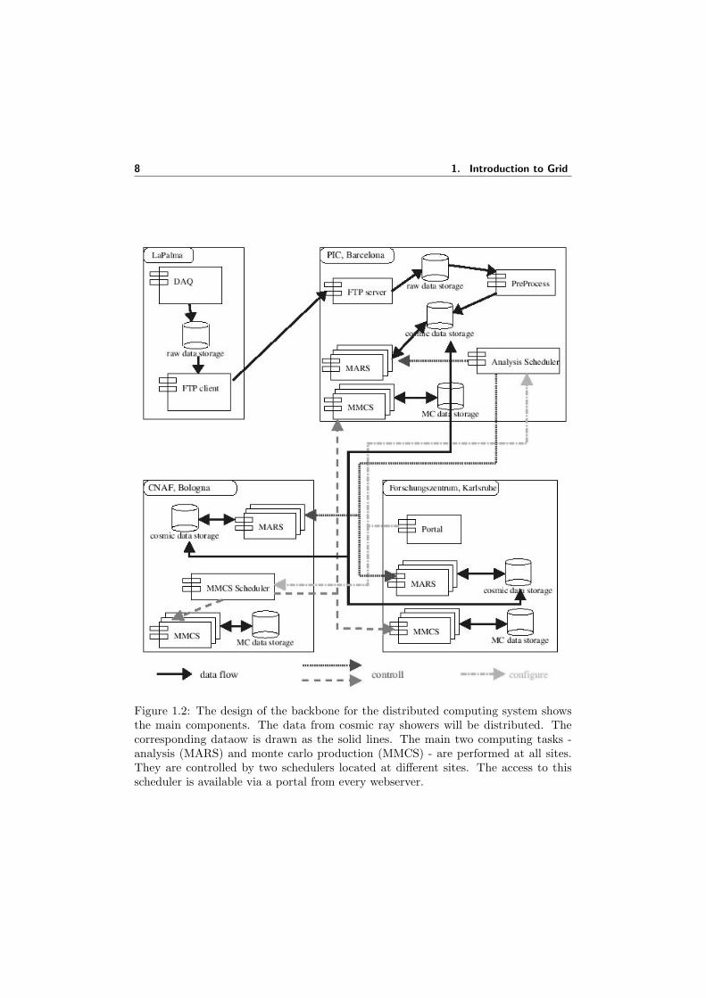
Figure 1.2 shows the computing centers that make available the main resources form-ing the backbone of the Grid system for MAGIC. These centers are: GRIDKA (Ger-many), CNAF (Italy) and PIC (Spain). The system [70] will be based on the middle-ware from the European Data Grid project [121], which is using the Globus toolkit[42] as the underlying software. The data flow starts in the island of La Palma andarrives in all the other centers passing through the PIC institute in Barcellona. Thetwo services of the system are the MAGIC Monte Carlo Simulation (MMCS) andthe MAGIC Analysis and Reconstruction Software (MARS). These services will runat all sites. Each of the two services will have its own scheduler (Resource Broker)running at CNAF or PIC. The schedulers will send the jobs to the different sites.The produced Monte Carlo data will be distributed as will the incoming real datafrom the telescope. The distribution and replication of the data will be based on thereplica location service of the EDG project. The system will be accessed via a portalrunning at GRIDKA. The local computers from a MAGIC partner site can connect tothe closest of the backbone nodes to contribute with their local computing resources.
1.3 Summary
Increased network bandwidth, more powerful computers, and the acceptance of theInternet have driven the on-going demand for new and better ways to compute. At theheart of Grid Computing is an infrastructure that provides dependable, consistent,pervasive and inexpensive access to computational capabilities. By pooling federatedassets into a virtual system, a grid provides a single point of access to powerfuldistributed resources. With a Grid, networked resources, e.g. desktops, servers,storage, databases, even scientific instruments, can be combined to deploy massivecomputing power wherever and whenever it is needed most. Users can find resourcesquickly, use them efficiently, and scale them seamlessly.
A Grid can be seen as the latest and most complete evolution f more familiardevelopments such as distributed computing, the Web, peer-to-peer computing and
8 1. Introduction to Grid
Figure 1.2: The design of the backbone for the distributed computing system showsthe main components. The data from cosmic ray showers will be distributed. Thecorresponding dataow is drawn as the solid lines. The main two computing tasks -analysis (MARS) and monte carlo production (MMCS) - are performed at all sites.They are controlled by two schedulers located at different sites. The access to thisscheduler is available via a portal from every webserver.
1.3. Summary 9
virtualization technologies. There are many challenges that must be addressed inorder to build a working Grid environment, such as: information services, resourcebrokering, uniform access to resources, security, job scheduling, data access and datareplication.
Grid is nowadays becoming a reality. Although it is at a very early stage of real-ization, many applications covering different research areas like experimental physics,astroparticle physics experiments, bioinformatics, earth observation, etc., are cur-rently migrating to Grid.

10 1. Introduction to Grid

2Grid technologies
There is much development work to be done in order to deploy a working Grid. How-ever, there has been a lot of work done in the past decade in the area of distributedcomputing and clearly it is essential to build on this wherever possible. Moreover,due to the rapid growth of the Internet and the Web, there has been a rising inter-est in Web-based distributed computing, and many projects have been started thataim to exploit the Web as an infrastructure for running coarse-grained distributedand parallel applications. In this context Grid is emerging as an Internet-based dis-tributed system. An increasing number of research groups have been working in thefield of wide-area distributed computing. These groups have implemented middle-ware, libraries and tools that allow the cooperative use of geographically distributedresources unified to act as a single powerful platform for the execution of a range ofparallel and distributed applications. This approach to computing has been known byseveral names, such as metacomputing, scalable computing, global computing, Inter-net computing and lately as Grid computing. This chapter presents an overview of thetechnologies, open standards and protocols used for building up this new paradigm.
2.1 Brief overview of distributed systems
A general and effective definition of distributed systems can be found in [118]: a dis-tributed system is a collection of independent computers that appears to its users as asingle coherent system. We can mention two important characteristics: the differencesbetween the various computers and the ways in which they communicate are hiddenfrom users and the users and the applications can interact with a distributed systemin a consistent and uniform way, regardless of where and when interaction takes place.
To support heterogeneous computers and networks while offering a single-systemview, distributed systems are often organized by means of a layer of software that islogically placed between a higher-level layer consisting of users and applications, anda layer underneath consisting of operating systems. This layer of software is calledmiddleware. There are many definitions of middleware. Practically, the middlewareis a connectivity software that consists of a set of enabling services that allow mul-tiple processes running on one or more machines to interact across a network. Thistechnology has evolved during the 1990’s to provide for interoperability in support
12 2. Grid technologies
of the move to client/server architectures. The most widely-publicized middlewareinitiatives are the Open Software Foundation’s Distributed Computing Environment(DCE), Object Management Group’s Common Object Request Broker Architecture(CORBA), and Microsoft’s COM/DCOM (COM, DCOM).
2.1.1 Properties of a distributed system
There are many possible ways to evaluate distributed systems. Here we present aset of properties that a distributed system should implement. While not exhaustive,this set is chosen because these properties are often used when talking about theadvantages or disadvantages of decentralized systems.
Security. A distributed system connects many users and resources and as this con-nectivity increases, security becomes more and more important. Security coversa variety of topics, such as preventing people from taking over the system, in-jecting bad information, or using the system for a purpose other than what theowners intend.
Transparency. A distributed system should hide the fact that its processes andresources are physically distributed across multiple computers. There are manykinds of transparency:
• Access transparency: hides differences in data representation and the waythat resources can be accessed by users.
• Location transparency: manages of names for accessing resources. A phys-ical or a logical name can be used.
• Migration transparency: manages the relocation of the resources.
• Relocation transparency: hides that a resource may be moved to anotherlocation while in use.
• Replication transparency: hides that a resource is replicated.
• Concurrency transparency: hides that a resource may be shared by severalcompetitive users.
• Failure transparency: hides the failure and recovery of a resource.
• Persistence transparency: hides whether a software resource is in memoryor on disk.
Openness. An open distributed system is a system that offers services according tostandard rules that describe the syntax and semantics of those services. Indistributed systems, services are generally specified through interfaces. Manyproblems must be addressed in order to build an open distributed system:
• Detailed interfaces of components need to be published.
• Flexibility: new components have to be integrated with existing compo-nents and it has to be easy to configure.
2.2. The client-server model 13
• Interoperability: two implementations of systems or components from dif-ferent manufactures can co-exist and work together by merely relying oneach others services as specified by a common standard.
• Portability: an application developed for a distributed system A can beexecuted, without modification, on a different distributed system B thatimplements the same interfaces as A.
Scalability. It indicates the capability of a system to increase total througput underan increased load when resources (typically hardware) are added. Scalability ofa system can be measured along at least three different dimensions [118, 96]:
• Size: more users and resources can be easily added to the system.
• Geographic: A geographically scalable system is one that maintains itsusefulness and usability, regardless of how far apart its users or resourcesare.
• Administrative: no matter how many different organizations need to sharea single distributed system, it should still be easy to use and manage.
2.2 The client-server model
Important to any distributed system is its internal organization. The client-servermodel is the most widely accepted model for structuring distributed systems. Abasic definition can be the following: client/server is a computational architecturethat involves client processes requesting service from server processes. A serveris a process implementing a specific service, for example, a file system service ora database service. A client is a process that requests a service from a server bysending it a request and subsequently waiting for the server’s reply. This interactionis also known as request-reply behavior. In general, client/server maintains adistinction between processes and network devices. Usually a client computer and aserver computer are two separate devices, each customized for their designed purpose.In any case, the same device may function as both client and server, hence, a devicethat is a server at one moment can reverse roles and become a client to a differentserver (either for the same application or for a different application).
Although communication between a client and a server can be implemented bymeans of a simple connectionless protocol (if the underlying network is fairly reliable),it is usually based on a reliable connection-oriented protocol, like the TCP/IP.
Advantages and disadvantages of the client-server model
The client-server model was originally developed to allow more users to share accessto database applications. Compared to the mainframe approach, client-server offersimproved scalability because connections can be made as needed rather than beinghard-wired. Flexible user interface development is the most obvious advantage ofclient-server computing. It is possible to create an interface that is independent of
14 2. Grid technologies
the server hosting the data. Therefore, the user interface of a client-server applicationcan be written on a Macintosh and the server can be written on a mainframe. Clientscould be also written for DOS- or UNIX-based computers. The client-server modelalso supports modular applications. In the so-called two-tier and three-tier types ofclient-server systems, a software application is separated into modular pieces, andeach piece is installed on hardware specialized for that subsystem.
One area of special concern in client-server networking is system management.With applications distributed across the network, it can be challenging to keep con-figuration information up-to-date and consistent among all of the devices. Therefore,upgrades to a newer version of a client-server application can be difficult to synchro-nize or stage appropriately. Finally, client-server systems rely heavily on the network’sreliability; redundancy or fail-over features can be expensive to implement.
2.3 Communication
Interprocess communication is at the heart of all distributed systems, and there aremany ways to exchange information among processes on different machines. In tradi-tional network applications, communication is often based on the low-level message-passing primitives offered by the transport layer. An important issue in middlewaresystems is to offer a higher level of abstraction that will make it easier to express com-munication between processes than the support offered by the interface to the trans-port layer. At least four abstractions can be distinguished: the Remote ProcedureCall (RPC), the Remote Object Invocation, the message-oriented communication andthe stream-oriented communication. We briefly describe these four communicationmethods.
2.3.1 Remote procedure call
Remote Procedure Call (RPC) is a powerful technique for constructing distributed,client-server based applications [118, 83]. It is based on extending the notion ofconventional, or local procedure calling, so that the called procedure need not existin the same address space as the calling procedure. The two processes may be on thesame system, or they may be on different systems with a network connecting them. Byusing RPC, programmers of distributed applications avoid the details of the interfacewith the network. The transport independence of RPC isolates the application fromthe physical and logical elements of the data communications mechanism and allowsthe application to use a variety of transports.
How RPC works
The idea is to make a remote procedure call look as much as possible like a local one, ithas to be transparent. In order to achieve this goal, client and server stubs are used.When the calling process calls a procedure, the action performed by that procedurewill not be the actual code as written, but code that begins network communication.
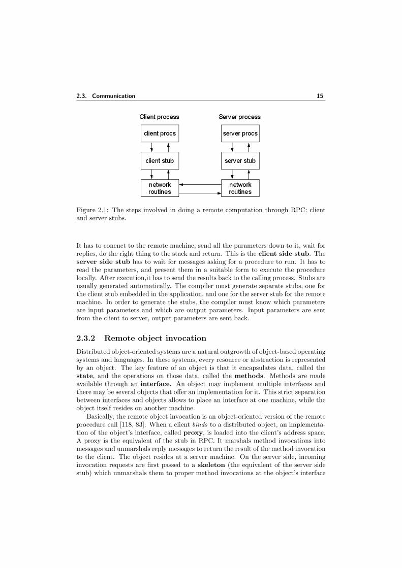
2.3. Communication 15
Figure 2.1: The steps involved in doing a remote computation through RPC: clientand server stubs.
It has to conenct to the remote machine, send all the parameters down to it, wait forreplies, do the right thing to the stack and return. This is the client side stub. Theserver side stub has to wait for messages asking for a procedure to run. It has toread the parameters, and present them in a suitable form to execute the procedurelocally. After execution,it has to send the results back to the calling process. Stubs areusually generated automatically. The compiler must generate separate stubs, one forthe client stub embedded in the application, and one for the server stub for the remotemachine. In order to generate the stubs, the compiler must know which parametersare input parameters and which are output parameters. Input parameters are sentfrom the client to server, output parameters are sent back.
2.3.2 Remote object invocation
Distributed object-oriented systems are a natural outgrowth of object-based operatingsystems and languages. In these systems, every resource or abstraction is representedby an object. The key feature of an object is that it encapsulates data, called thestate, and the operations on those data, called the methods. Methods are madeavailable through an interface. An object may implement multiple interfaces andthere may be several objects that offer an implementation for it. This strict separationbetween interfaces and objects allows to place an interface at one machine, while theobject itself resides on another machine.
Basically, the remote object invocation is an object-oriented version of the remoteprocedure call [118, 83]. When a client binds to a distributed object, an implementa-tion of the object’s interface, called proxy, is loaded into the client’s address space.A proxy is the equivalent of the stub in RPC. It marshals method invocations intomessages and unmarshals reply messages to return the result of the method invocationto the client. The object resides at a server machine. On the server side, incominginvocation requests are first passed to a skeleton (the equivalent of the server sidestub) which unmarshals them to proper method invocations at the object’s interface
16 2. Grid technologies
at the server.Usually it is only the interface of an object to be distributed, the state is not
distributed and resides at a single machine. Such objects are also referred to asremote objects. It is however possible to find objects whose state may be distributedacross multiple machines, and this distribution is also hidden from clients behind theobject’s interfaces.
2.3.3 Message-oriented communication
Message-oriented communication is a way of communicating between processes. Mes-sages, which correspond to events, are the basic units of data delivered. Tanenbaumand Steen [118] classified message-oriented communication according to two factors:synchronous or asynchronous communication, and transient or persistent communi-cation. In synchronous communication, the sender blocks waiting for the receiverto engage in the exchange. Asynchronous communication does not require both thesender and the receiver to execute simultaneously. So, the sender and recipient areloosely-coupled. The amount of time messages are stored determines whether thecommunication is transient or persistent. Transient communication stores the mes-sage only while both partners in the communication are executing. If the next routeror receiver is not available, then the message is discarded. Persistent communication,on the other hand, stores the message until the recipient receives it.
There are several combinations of these types of communication that occur inpractice. Examples of message oriented transient communication are the BerkleySockets and the Message Passing Interface (MPI). On the other side, a typical ex-ample of asynchronous persistent communication is Message-Oriented Middleware(MOM). Message-oriented middleware is also called a message-queuing system, a mes-sage framework, or just a messaging system. MOM can form an important middlewarelayer for enterprise applications on the Internet. In the publish and subscribe model(see 2.4.1), a client can register as a publisher or a subscriber of messages. Messagesare delivered only to the relevant destinations and only once, with various communi-cation methods including one-to-many or many-to-many communication. The datasource and destination can be decoupled under such a model.
2.3.4 Stream-oriented communication
Communication as discussed so far was based on:
• independent and complete units of information;
• moment of receiving is not important for correctness.
There are some situations where communication timing plays a crucial role. For ex-ample, in a real time video conference moment of receiving and correct representationare essential. To capture the exchange of time-dependent information, distributedsystems generally provide support for data streams, which are sequence of dataunits. Regarding on how timing is considered, three different transmission modes canbe distinguished:
2.4. Service Oriented Architecture 17
• Asynchronous transmission mode: no timing constraints, data items are trans-mitted one after the other. File transmission is a typical example.
• Synchronous transmission mode: there is a maximum end-to-end delay for eachunit in a data stream.
• Isochronous transmission mode: data transfer is subject to a maximum andminimum end-to-end delay, also referred to as bounded jitter. The term streamsusually identifies continuous data streams using isochronous transmission.
A stream can be simple or complex, depending if it consists of only a single sequenceof data or several related simple streams (e.g. stereo audio, audio and video). Sub-streams of complex streams must be continuously synchronized. A stream can oftenbe considered as a virtual connection between a source and a sink. The source or sinkcan be a process, but could also be a device. Time-dependent (and other nonfunc-tional) requirements are generally expressed as Quality of Service (QoS) requirements.These requirements describe what is needed from the underlying distributed systemand network to ensure that, for example, the temporal relationships in a stream canbe preserved.
2.4 Service Oriented Architecture
This and the next section want to introduce the basic concepts on which Grid is beingtaking form. The first fact is that Grid is evolving into a Service Oriented Architecture(SOA), primarily based on Web Services. The SOA is based on the concept of loosecoupling. Coupling is the dependency between interacting systems. This dependencycan be decomposed into real dependency and artificial dependency:
1. Real dependency is the set of features or services that a system consumes fromother systems. The real dependency always exists and cannot be reduced.
2. Artificial dependency is the set of factors that a system has to comply with inorder to consume the features or services provided by other systems. Typicalartificial dependency factors are language dependency, platform dependency,API dependency, etc. Artificial dependency always exists, but it or its cost canbe reduced.
For example, if you travel overseas on business, you know that you must bring poweradapters along with you. The real dependency is that you need power; the artificialdependency is that your plug must fit into the local outlet. Looking at all the varyingsizes and shapes of those plugs from different countries, you would notice that someof them are small and compact while many others are big and bulky. We cannotremove artificial dependencies, but we can reduce them. If the artificial dependenciesamong systems have been reduced, ideally, to their minimum, we have achieved loosecoupling.
SOA is an architectural style whose goal is to achieve loose coupling among in-teracting software agents. A service is a unit of work done by a service provider to
18 2. Grid technologies
Figure 2.2: Elements of the Service Oriented Architecture
achieve desired end results for a service consumer. Both provider and consumer areroles played by software agents on behalf of their owners. How does SOA achieve loosecoupling among interacting software agents? It does so by employing two architecturalconstraints:
1. A small set of simple and ubiquitous interfaces to all participating softwareagents. Only generic semantics are encoded at the interfaces. The interfacesshould be universally available for all providers and consumers.
2. Descriptive messages constrained by an extensible schema delivered through theinterfaces. No, or only minimal, system behavior is prescribed by messages. Aschema limits the vocabulary and structure of messages. An extensible schemaallows new versions of services to be introduced without breaking existing ser-vices.
Since we have only a few generic interfaces available, we must express application-specific semantics in messages. We can send any kind of message over our interfaces,but there are a few rules to follow before we can say that an architecture is serviceoriented. First, the messages must be descriptive, rather than instructive, because theservice provider is responsible for solving the problem. Second, service providers willbe unable to understand your request if your messages are not written in a format,structure, and vocabulary that is understood by all parties. Limiting the vocabularyand structure of messages is a necessity for any efficient communication. The morerestricted a message is, the easier it is to understand the message, although it comesat the expense of reduced extensibility. Third, extensibility is vitally important. Ifmessages are not extensible, consumers and providers will be locked into one particularversion of a service.
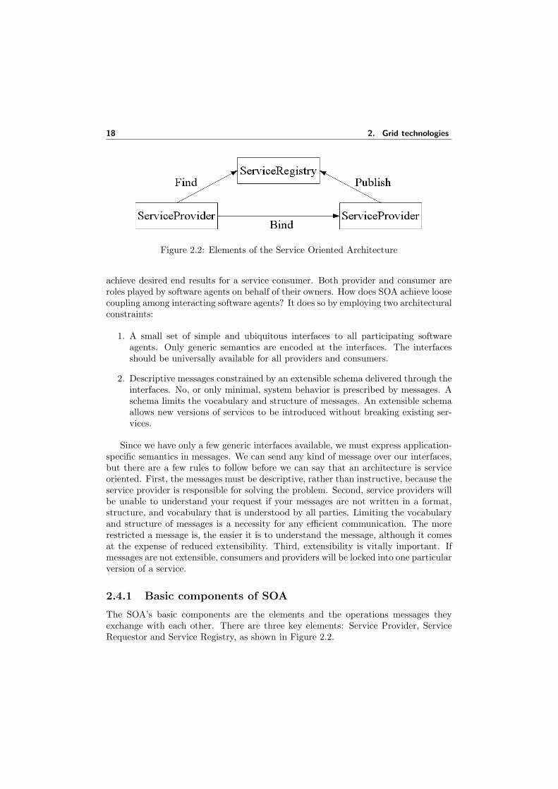
2.4.1 Basic components of SOA
The SOA’s basic components are the elements and the operations messages theyexchange with each other. There are three key elements: Service Provider, ServiceRequestor and Service Registry, as shown in Figure 2.2.

2.4. Service Oriented Architecture 19
Service Provider. The Service Provider is responsible for building a useful service,creating a service description for it, publishing that service description to oneor more service registries, and receiving service invocation messages from oneor more Service Requestors.
Service Requestor. The Service Requestor is responsible for finding a service de-scription published to one or more Service Registries, such as yellow pages forservices, and for using service descriptions to bind to or invoke services hostedby Service Providers. Any consumer of a service can be considered a ServiceRequestor.
Service Registry. The Service Registry is responsible for advertising service de-scriptions published to it by the Service Providers, and for allowing ServiceRequestors to search the collection of service descriptions contained within theService Registry. Once the Service Registry provides a match between the Ser-vice Requestor and the Service Provider, the Service Registry is no longer neededfor the interaction.
Operations are defined by contracts between the above elements. There are threetypes of contracts: Publish, Find and Bind, as shown in Figure 2.2.
Publish. The Publish operation is a contract between the Service Provider and theService Registry. The Service Provider registers the service interfaces it providesat the Service Registry using the Publish operation. Once published, the servicesprovided by the Service Provider are available for any Service Requestor to use.
Find. The Find operation is a contract between the Service Requestor and ServiceRegistry. The Service Requestor uses the Find operation to get a list of theService Providers that satisfies its needs. It may indicate one or more searchcriteria, such as the desired availability and performance, in the Find operation.The Service Registry searches through all the registered Service Providers andreturns the appropriate information.
Bind. The Bind operation is a contract between the Service Requestor and the Ser-vice Provider. It allows the Service Requestor to connect to the Service Providerbefore invoking the operations. It also enables the Service Requestor to generatethe client-side proxy for the service provided by the Service Provider. The bind-ing can be dynamic or static: in the first case, the Service Requestor generatesthe client-side proxy based on the service description obtained from the ServiceRegistry at the time the service is invoked; the other case involves the ServiceRequestor generating the client-side proxy during application development.
2.4.2 Web services as an implementation of the SOA
The W3C (World Wide Web Consortium, which develops interoperable technologies,e.g. specifications, guidelines, software, and tools, to lead the Web to its full potential)[122] gives the following definition of web service:
20 2. Grid technologies
A Web service is a software system designed to support interoperablemachine-to-machine interaction over a network. It has an interface de-scribed in a machine-processable format (specifically WSDL). Other sys-tems interact with the Web service in a manner prescribed by its descrip-tion using SOAP messages, typically conveyed using HTTP with an XMLserialization in conjunction with other Web-related standards.
Several characteristics of a web service can be identified [19]:
XML based: XML is used as the data representation layer for all web services pro-tocols and technologies.
Loosely coupled: a consumer of a web service is not tied to that web service directly;the web service interface can change over time without compromising the client’sability to interact with the service.
Coarse-grained: object-oriented technologies expose their services through individ-ual methods. Building a program from scratch requires the creation of severalfine-grained methods that are then composed into a coarse-grained service thatis consumed by either a client or another service. Web services technologyprovides a natural way of defining coarse-grained services.
Ability to be synchronous or asynchronous: synchronicity refers to the bind-ing of the client to the execution of the service. In synchronous invocations,the client blocks and waits for the service to complete its operation before con-tinuing. Asynchronous operations allow a client to invoke a service and thenexecute other functions.
Supports Remote Procedure Calls (RPCs): web services allow clients to in-voke procedures, functions, and methods on remote objects using an XML-basedprotocol.
Supports document exchange: One of the key advantages of XML is its genericway of representing not only data, but also complex documents. Web servicessupport the transparent exchange of documents to facilitate business integra-tion.
Over the past two years, three primary technologies have emerged as worldwidestandards that make up the core of today’s web services technology. These tech-nologies are: SOAP, WSDL and UDDI. The Simple Object Access Protocol (SOAP)provides a standard packaging structure to transport XML documents over a varietyof standard Internet technologies, including SMTP, HTTP, and FTP. It is used toexchange messages between Web services. The Web Service Description Language(WSDL) is an XML technology that describes the interface of a web service in astandardized way and allows disparate clients to automatically understand how tointeract with a web service. The Universal Description, Discovery, and Integration(UDDI) provides a worldwide registry of web services for advertisement, discovery,
2.5. The evolution of the Grid 21
and integration purposes. One of the big promises of web services is seamless, au-tomatic business integration: a piece of software will discover, access, integrate, andinvoke new services from unknown companies dynamically without the need for hu-man intervention.
The web services model lends itself well to a highly distributed, service-orientedarchitecture (SOA). A web service may communicate with a handful of standaloneprocesses and functions or participate in a complicated, orchestrated business pro-cess. A web service can be published, located, and invoked within the enterprise, oranywhere on the Web.
2.5 The evolution of the Grid
Three stages of Grid evolution can be identified [106]: first-generation systems bornin the early to mid 1990s, second-generation systems with a focus on middlewareto support large-scale data and computation and current third-generation systemsin which the emphasis shifts to distributed global collaboration, a service-orientedapproach and information layer issues. The first generation marked the emergenceof the early metacomputing or Grid environments. Typically, the objective of theseearly metacomputing projects was to provide computational resources to a range ofhigh-performance applications. Two representative projects in the vanguard of thistype of technology were FAFNER [36] and I-WAY [41]. FAFNER was the forerunnerof the likes of SETI@home [112] and Distributed.Net [95], and I-WAY for Globus [42]and Legion [59]. The emphasis of the early efforts in Grid computing was in partdriven by the need to link a number of US national supercomputing centers.
The second-generation Grid was the result of the emergence of an infrastructurecapable of binding together more than just a few specialised supercomputing centers.Now the take-up of high bandwidth network technologies and adoption of standards,allows the Grid to be viewed as a viable distributed infrastructure on a global scalethat can support diverse applications requiring large-scale computation and data [43].There are three main issues that had to be confronted: heterogeneity, scalability andadaptability. In a Grid, the middleware is used to hide the heterogeneous nature ofthe resources and to provide users and applications with a homogeneous and seam-less environment by providing a set of standardised interfaces to a variety of ser-vices. Systems use varying standards and system application programming interfaces(APIs), resulting in the need to port services and applications to the plethora of com-puter systems used in a Grid environment. The most significant projects that havecontributed to make the Grid concrete are: Globus [42], Legion [59], the EuropeanDataGrid project [121], the UNIform Interface to COmputer REsources (UNICORE)project [7], the Cactus project [6], as well as others.
With third generation there is an increasing adoption of a service-oriented modeland increasing attention to metadata. There is a strong sense of automation in third-generation systems; for example, when humans can no longer deal with the scale andheterogeneity but delegate to processes to do so (e.g. through scripting), which leadsto autonomy within the systems. Similarly, the increased likelihood of failure implies
22 2. Grid technologies
a need for automatic recovery: configuration and repair cannot remain manual tasks.In the next section we describe the main characteristics of the Globus toolkit,
which is the standard de facto for the Grid middleware.
2.6 The Globus Toolkit
The Globus Toolkit [42] is actually the de facto standard middleware for Grid com-puting. It is a metacomputing infrastructure toolkit providing basic capabilities andinterfaces in areas such as communication, information, resource location, resourcescheduling, authentication, and data access. Together, these toolkit components de-fine a metacomputing abstract machine on which a range of alternative infrastructurescan be constructed, services, and applications. The term metacomputer is used todenote a networked virtual supercomputer, constructed dynamically from geographi-cally distributed resources linked by high-speed networks.
With version 3.0, the Globus Toolkit is a reference implementation of the OpenGrid Service Architecture (OGSA) published by the Global Grid Forum (GGF). It isdivided in four main components:
• The Grid Security Infrastructure.
• The resource management infrastructure (GRAM)
• The information management infrastructure.
• The data management infrastructure.
Globus Grid Security Infrastructure (GSI) Since a Grid implies crossing or-ganizational boundaries, resources are going to be accessed by many different organi-zations. This poses a lot of challenges:
• We have to make sure that only certain organizations can access our resources,and that we’re 100% sure that those users are really who they claim to be.In other words, we have to make sure that everyone in a Grid application isproperly authenticated/authorized;
• We are going to bump into some pretty interesting scenarios. For example,suppose organization A asks B to perform a certain task. B, on the other hand,realizes that the task should be delegated to organization C. However, let’ssuppose C only trusts A (and not B). Should C turn down the request becauseit comes from B, or accept it since the ’original’ requestor is A?
• Depending on the application, we may also be interested in assuring data in-tegrity and privacy, although in a Grid application this is generally not as im-portant as authentication.
The GSI offers the following three features:
• A complete public-key infrastructure.
2.6. The Globus Toolkit 23
• Mutual authentication through digital certificates.
• Credential delegation and single sign-on.
The GSI [129] is based on public-key cryptography, and therefore can be configured toguarantee privacy, integrity, and authentication. Mutual authentication is achievedusing X.509 certificates [128]. Grid is a collection of heterogeneous resources thatspan across multiple organization domains. In this context the single sign-on is a veryimportant feature. Situations like the one described before, where a job encompassesthree different organizations, are addressed with delegation. For example, it wouldinteresting to find a legitimate way for B to demonstrate that it is, in fact, acting onA’s behalf. One way of doing this would be for A to ’lend’ its public and private keypair to B. However, this is absolutely out of the question. Remember, the private keyhas to remain secret, and sending it to another organization (no matter how much youtrust them) is a big breach in security. What can be used, instead, are certificates.
The Globus Resource Allocation Manager Globus is a layered architecturein which high-level global services are built on top of an essential set of core localservices. At the bottom of this layered architecture, the Globus Resource AllocationManager (GRAM) [27] provides the local component for resource management. EachGRAM is responsible for a set of resources operating under the same site-specificallocation policy, often implemented by a local resource management system, such asLoad Sharing Facility (LSF) or Condor. GRAM provides a standard network-enabledinterface to local resource management systems. Hence, computational Grid toolsand applications can express resource allocation and process management requests interms of a standard application programming interface (API), while individual sitesare not constrained in their choice of resource management tools.
The Resource Specification Language (RSL) is used throughout this architecture asa common notation for expressing resource requirements. A variety of resource brokersimplement domain-specific resource discovery and selection policies by transformingabstract RSL expressions into progressively more specific requirements until a specificset of resources is identified.The final step in the resource allocation process is todecompose the RSL into a set of separate resource allocation requests and to dispatcheach request to the appropriate GRAM.
The Globus Information Management The dynamic nature of Grid environ-ments means that toolkit components, programming tools, and applications must beable to adapt their behavior in response to changes in system structure and state [26].Globus Metacomputing Directory Service (MDS) is designed to support this type ofadaptation by providing an information-rich environment in which information aboutsystem components is always available. MDS stores and makes accessible informationsuch as the architecture type, operating system version and amount of memory on acomputer, network bandwidth and latency, available communication protocols, andthe mapping between IP addresses and network technology.
24 2. Grid technologies
An information-rich environment is more than just mechanisms for naming anddisseminating information: it also requires agents that produce useful information andcomponents that access and use that information. Within Globus, both these rolesare distributed over every system component and potentially over every application.Every Globus service is responsible for producing information that users of that servicemay find useful, and for using information to enhance its flexibility and performance.
The Globus Data Management The main components of the data managementinfrastructure are:
GridFTP. It is a high-performance, secure protocol based on the Internet Engineer-ing Task Force’s FTP standards which uses the GSI (Grid Security Infrastruc-ture) for authentication and new extensions to the FTP protocol for paralleldata transfer, partial file transfer, and third-party (server-to-server) data trans-fer [5]. This will allow Grid applications to have ubiquitous, high-performanceaccess to data in a way that is compatible with the most popular file transferprotocol in use today.
Data Replication. Tools for managing data replicas: multiple copies of data storedin different systems to improve access across geographically-distributed Gridsand fault-tolerance [20]. These replication technologies currently include aReplica Catalog (that stores information about files and their replicas) anda Replica Management tool that combines the Replica Catalog with GridFTPto manage data replication.
2.7 Open Grid Service Architecture (OGSA)
A wide array of heterogeneous resources comprise a Grid, and it’s important thatthey interact and behave in well-known and consistent ways. The need for open stan-dards that define this interaction and encourage interoperability between componentssupplied from different sources was the motivation for the Open Grid Services Ar-chitecture (OGSA) [44], specified by the Open Grid Services Infrastructure workinggroup of the Global Grid Forum (GGF) in June 2002. The objectives of OGSA are:
• Manage resources across distributed heterogeneous platforms.
• Deliver seamless quality of service (QoS). The topology of Grids is often com-plex. Interaction of Grid resources is usually dynamic. It’s important that theGrid provide robust, behind-the-scenes services such as authorization, accesscontrol, and delegation.
• Provide a common base for autonomic management solutions. A Grid cancontain many resources, with numerous combinations of configurations, inter-actions, and changing state and failure modes. Some form of intelligent selfregulation and autonomic management of these resources is necessary.
2.7. Open Grid Service Architecture (OGSA) 25
Figure 2.3: Elements of the Service Oriented Architecture
• Define open, published interfaces. OGSA is an open standard managed by theGGF standards body. For interoperability of diverse resources, Grids must bebuilt on standard interfaces and protocols.
• Exploit industry standard integration technologies.
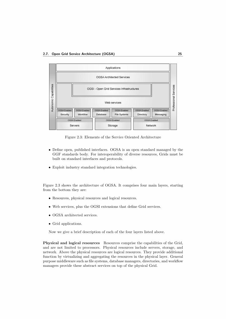
Figure 2.3 shows the architecture of OGSA. It comprises four main layers, startingfrom the bottom they are:
• Resources, physical resources and logical resources.
• Web services, plus the OGSI extensions that define Grid services.
• OGSA architected services.
• Grid applications.
Now we give a brief description of each of the four layers listed above.
Physical and logical resources Resources comprise the capabilities of the Grid,and are not limited to processors. Physical resources include servers, storage, andnetwork. Above the physical resources are logical resources. They provide additionalfunction by virtualizing and aggregating the resources in the physical layer. Generalpurpose middleware such as file systems, database managers, directories, and workflowmanagers provide these abstract services on top of the physical Grid.
26 2. Grid technologies
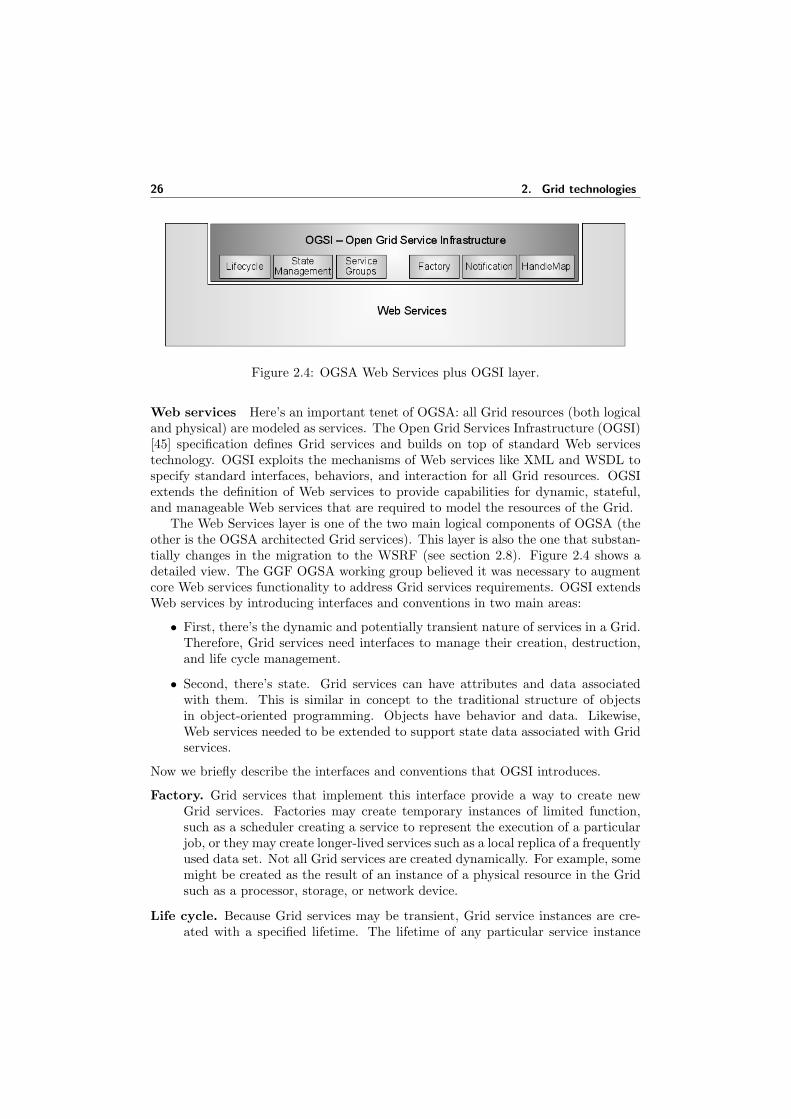
Figure 2.4: OGSA Web Services plus OGSI layer.
Web services Here’s an important tenet of OGSA: all Grid resources (both logicaland physical) are modeled as services. The Open Grid Services Infrastructure (OGSI)[45] specification defines Grid services and builds on top of standard Web servicestechnology. OGSI exploits the mechanisms of Web services like XML and WSDL tospecify standard interfaces, behaviors, and interaction for all Grid resources. OGSIextends the definition of Web services to provide capabilities for dynamic, stateful,and manageable Web services that are required to model the resources of the Grid.
The Web Services layer is one of the two main logical components of OGSA (theother is the OGSA architected Grid services). This layer is also the one that substan-tially changes in the migration to the WSRF (see section 2.8). Figure 2.4 shows adetailed view. The GGF OGSA working group believed it was necessary to augmentcore Web services functionality to address Grid services requirements. OGSI extendsWeb services by introducing interfaces and conventions in two main areas:
• First, there’s the dynamic and potentially transient nature of services in a Grid.Therefore, Grid services need interfaces to manage their creation, destruction,and life cycle management.
• Second, there’s state. Grid services can have attributes and data associatedwith them. This is similar in concept to the traditional structure of objectsin object-oriented programming. Objects have behavior and data. Likewise,Web services needed to be extended to support state data associated with Gridservices.
Now we briefly describe the interfaces and conventions that OGSI introduces.
Factory. Grid services that implement this interface provide a way to create newGrid services. Factories may create temporary instances of limited function,such as a scheduler creating a service to represent the execution of a particularjob, or they may create longer-lived services such as a local replica of a frequentlyused data set. Not all Grid services are created dynamically. For example, somemight be created as the result of an instance of a physical resource in the Gridsuch as a processor, storage, or network device.
Life cycle. Because Grid services may be transient, Grid service instances are cre-ated with a specified lifetime. The lifetime of any particular service instance
2.8. Web Services Resource Framework 27
can be negotiated and extended as required by components that are dependenton or manage that service. The life cycle mechanism was architected to preventGrid services from consuming resources indefinitely without requiring a largescale distributed ”garbage collection” scavenger.
State management. Grid services can have state. OGSI specifies a framework forrepresenting this state called Service Data and a mechanism for inspecting ormodifying that state named Find/SetServiceData.
Service groups. Service groups are collections of Grid services that are indexed,using Service Data, for some particular purpose. For example, they might beused to collect all the services that represent the resources in a particular cluster-node within the Grid.
Notification. The state information (Service Data) that is modeled for Grid ser-vices changes as the system runs. Many interactions between Grid servicesrequire dynamic monitoring of changing state. Notification applies a traditionalpublish/subscribe paradigm to this monitoring. Grid services support an in-terface (NotificationSource) to permit other Grid services (NotificationSink) tosubscribe to changes.
HandleMap. When factories are used to create a new instance of a Grid service,the factory returns the identity of the newly instantiated service. This identityis composed of two parts, a Grid Service Handle (GSH) and a Grid ServiceReference (GSR). A GSH is guaranteed to reference the Grid service indefinitely,while a GSR can change within the Grid services lifetime. The HandleMapinterface provides a way to obtain a GSR given a GSH. This might seem simple,but there are a number of associated intricacies with such a request [44].
OGSA architected Grid services The previous layer, Web services with its OGSIextensions, provide a base infrastructure for this layer. The Global Grid Forumis currently working to define many of these architected Grid services in areas likeprogram execution, data services, and core services (Figure 2.5). Some are alreadydefined, and some implementations have already appeared. As implementations ofthese newly architected services begin to appear, OGSA will become a more usefulservice-oriented architecture (SOA).
Grid applications Over time, as a rich set of Grid-architected services continuesto be developed, new Grid applications that use one or more Grid architected serviceswill appear.
2.8 Web Services Resource Framework
In January 2004, the WS-Resource Framework (WSRF) was presented, an open frame-work for modeling and accessing stateful resources using Web services. WSRF defines
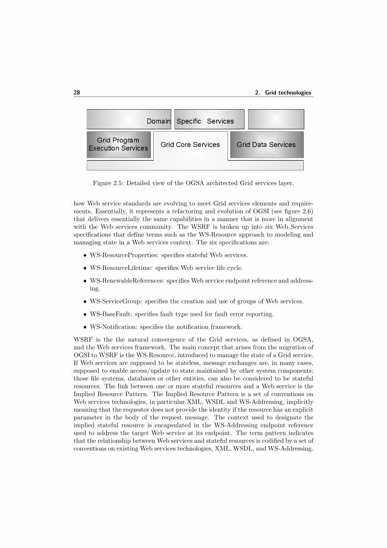
28 2. Grid technologies
Figure 2.5: Detailed view of the OGSA architected Grid services layer.
how Web service standards are evolving to meet Grid services elements and require-ments. Essentially, it represents a refactoring and evolution of OGSI (see figure 2.6)that delivers essentially the same capabilities in a manner that is more in alignmentwith the Web services community. The WSRF is broken up into six Web Servicesspecifications that define terms such as the WS-Resource approach to modeling andmanaging state in a Web services context. The six specifications are:
• WS-ResourceProperties: specifies stateful Web services.
• WS-ResourceLifetime: specifies Web service life cycle.
• WS-RenewableReferences: specifies Web service endpoint reference and address-ing.
• WS-ServiceGroup: specifies the creation and use of groups of Web services.
• WS-BaseFault: specifies fault type used for fault error reporting.
• WS-Notification: specifies the notification framework.
WSRF is the the natural convergence of the Grid services, as defined in OGSA,and the Web services framework. The main concept that arises from the migration ofOGSI to WSRF is the WS-Resource, introduced to manage the state of a Grid service.If Web services are supposed to be stateless, message exchanges are, in many cases,supposed to enable access/update to state maintained by other system components;those file systems, databases or other entities, can also be considered to be statefulresources. The link between one or more stateful resources and a Web service is theImplied Resource Pattern. The Implied Resource Pattern is a set of conventions onWeb services technologies, in particular XML, WSDL and WS-Addressing, implicitlymeaning that the requestor does not provide the identity if the resource has an explicitparameter in the body of the request message. The context used to designate theimplied stateful resource is encapsulated in the WS-Addressing endpoint referenceused to address the target Web service at its endpoint. The term pattern indicatesthat the relationship between Web services and stateful resources is codified by a set ofconventions on existing Web services technologies, XML, WSDL, and WS-Addressing.
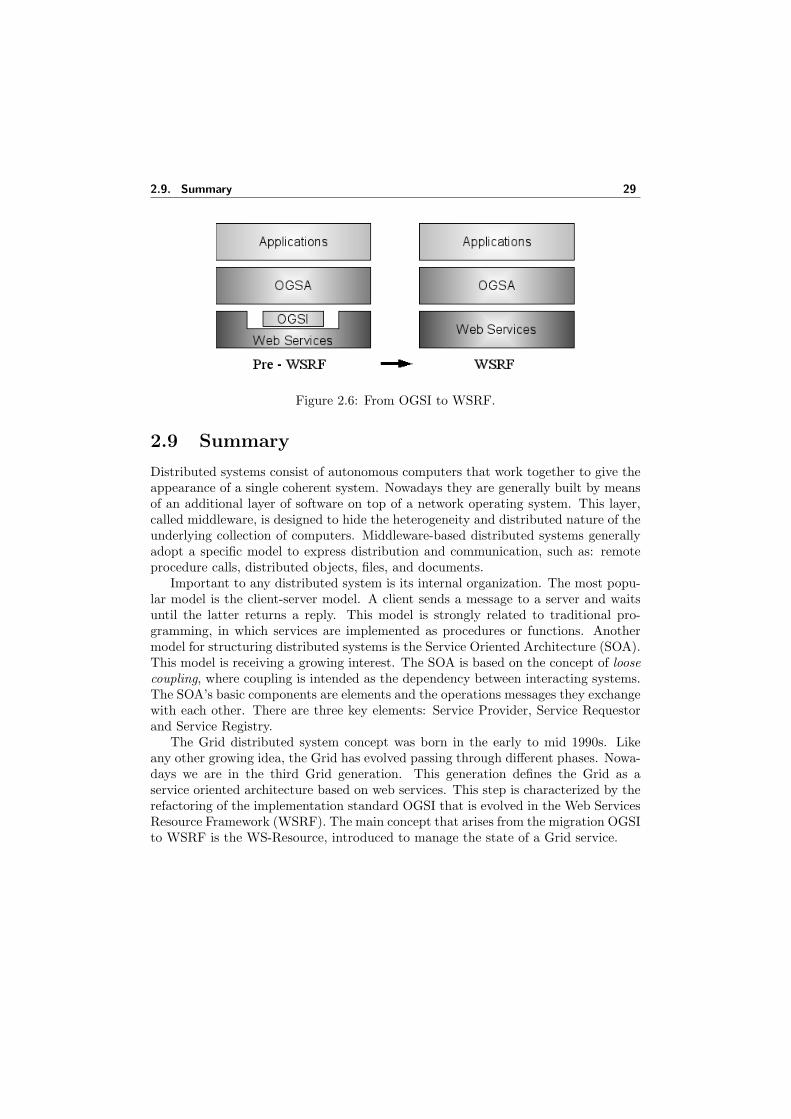
2.9. Summary 29
Figure 2.6: From OGSI to WSRF.
2.9 Summary
Distributed systems consist of autonomous computers that work together to give theappearance of a single coherent system. Nowadays they are generally built by meansof an additional layer of software on top of a network operating system. This layer,called middleware, is designed to hide the heterogeneity and distributed nature of theunderlying collection of computers. Middleware-based distributed systems generallyadopt a specific model to express distribution and communication, such as: remoteprocedure calls, distributed objects, files, and documents.
Important to any distributed system is its internal organization. The most popu-lar model is the client-server model. A client sends a message to a server and waitsuntil the latter returns a reply. This model is strongly related to traditional pro-gramming, in which services are implemented as procedures or functions. Anothermodel for structuring distributed systems is the Service Oriented Architecture (SOA).This model is receiving a growing interest. The SOA is based on the concept of loosecoupling, where coupling is intended as the dependency between interacting systems.The SOA’s basic components are elements and the operations messages they exchangewith each other. There are three key elements: Service Provider, Service Requestorand Service Registry.
The Grid distributed system concept was born in the early to mid 1990s. Likeany other growing idea, the Grid has evolved passing through different phases. Nowa-days we are in the third Grid generation. This generation defines the Grid as aservice oriented architecture based on web services. This step is characterized by therefactoring of the implementation standard OGSI that is evolved in the Web ServicesResource Framework (WSRF). The main concept that arises from the migration OGSIto WSRF is the WS-Resource, introduced to manage the state of a Grid service.

30 2. Grid technologies
3Grid scheduling
A Grid is a dynamic heterogeneous environment that agglomerates geographicallydistributed resources. Therefore, a Grid scheduler (or broker) must make resourceselection decisions in an environment where it has no control over the local resources,the resources are distributed, and information about the systems is often limited ordated. These interactions are also closely tied to the functionality of the Grid Infor-mation Services. In this chapter we describe properties and services characterizingthe Grid Resource Management System (RMS), that provides services for the man-agement and exploitation of the resources (scheduling services are part of the RMS).Then we tackle the problem of scheduling applications in a Grid environment andgive a brief summary of current projects dealing with Grid scheduling systems.
3.1 Grid Resource Management Systems
Grid is a large, dynamic, heterogeneous and collaborative environment. Grids inte-grate networking, communication, computation and information to provide a virtualplatform for computing and data management. Machines in a Grid are typicallygrouped into autonomous administrative domains that communicate via high-speedcommunication links. Scheduling, in such an environment, requires a different ap-proach than presently used in distributed systems. This approach must take intoaccount that resources in a Grid typically do not belong to the same administrativedomain. Therefore, the individual demands of the participants need to be observed.This requires a new technological approach. Access to resources is typically subjectto individual access, accounting, priority, and security policies of the resource owners.Moreover a Grid resource is a very general concept, it is not restricted only to CPUcycles, but also network bandwidth, disk space, memory, files, etc. In a broad sensea Grid resource is anything that may be used through a standard Grid interface, i.e.an Application Programming Interface and a protocol.
In a Grid environment there is the need of a set of basic functions and servicesthat take care of all these constraints, that means accepting requests for resourcesand assign specific machine resources to a request from the overall pool of Grid re-sources for which a user has access permission. This set of services is called GridResource Management System (RMS). The RMS manages the pool of resources that
32 3. Grid scheduling
are available to the Grid, i.e. the scheduling of processors, network bandwidth, anddisk storage. In a Grid, the pool can include resources from different providers thusrequiring the RMS to hold the trust of all resource providers. Basically, the RMS isconstituted by the middleware, tools and services that allow to disseminate resourceinformation, discover suitable resources and scheduling resources for job execution.The design of a RMS have to consider aspects such as: site autonomy, heterogeneity,extensibility, allocation/co-allocation, scheduling, and online control [45, 26, 10].
Site autonomy. Computing resources are geographically distributed under differentownerships each having their own access policy, cost and various constraints.Every resource owner will have a unique way of managing and scheduling re-sources and the Grid schedulers have to ensure that they do not conflict withresource owners policies.
Heterogeneity. The solution of complex problems can require various kind of re-sources located on different sites that can use different operating systems aswell as different local resource management systems which lead to significantdifferences in functionality.
Extensibility. A resource management solution must support the frequent develop-ment of new domain-specific management structures, without requiring changesto code installed at participating sites.
Allocation/Co-allocation. Applications have computational requirements that canbe satisfied by using one or more resources that could be allocated simultane-ously at several sites. Site autonomy and possibility of failure during allocationintroduces a need for specialized mechanisms for allocating resources, initiatingcomputation on those resources, and monitoring and managing those computa-tions.
Scheduling. To achieve high performance, efficient mechanism to assign job/appli-cations tasks to the selected resources and to schedule on them their executionare needed.
Online control. Many applications can require to adapt their execution to resourceavailability, in particular when application requirements and resource charac-teristics change during application execution.
In the past several RMS were proposed, but currently no one supports a full set offunctionalities as required by a Grid RMS. For example, Condor [14] supports site au-tonomy, but not co-allocation or online control, others, such as Legion, supports onlinecontrol and policy extensibility, but not the heterogeneous substrate or co-allocationproblems [30]. In [109] a taxonomy to survey existing Grid resource managementimplementations can be found.
Any application can be a Grid application but, in order to take full advantagefrom the Grid, it should be based on loosely-coupled components and it should beGrid-aware, i.e. designed to work in Grid. A Grid-aware application is one that at
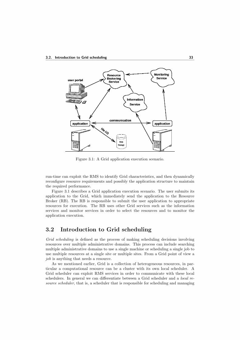
3.2. Introduction to Grid scheduling 33
Figure 3.1: A Grid application execution scenario.
run-time can exploit the RMS to identify Grid characteristics, and then dynamicallyreconfigure resource requirements and possibly the application structure to maintainthe required performance.
Figure 3.1 describes a Grid application execution scenario. The user submits itsapplication to the Grid, which immediately send the application to the ResourceBroker (RB). The RB is responsible to submit the user application to appropriateresources for execution. The RB uses other Grid services such as the informationservices and monitor services in order to select the resources and to monitor theapplication execution.
3.2 Introduction to Grid scheduling
Grid scheduling is defined as the process of making scheduling decisions involvingresources over multiple administrative domains. This process can include searchingmultiple administrative domains to use a single machine or scheduling a single job touse multiple resources at a single site or multiple sites. From a Grid point of view ajob is anything that needs a resource.
As we mentioned earlier, Grid is a collection of heterogeneous resources, in par-ticular a computational resource can be a cluster with its own local scheduler. AGrid scheduler can exploit RMS services in order to communicate with these localschedulers. In general we can differentiate between a Grid scheduler and a local re-source scheduler, that is, a scheduler that is responsible for scheduling and managing

34 3. Grid scheduling
resources at a single site, or perhaps only for a single cluster or resource. One of theprimary differences between a Grid scheduler and a local resource scheduler is thatthe Grid scheduler does not own the resources at a site (unlike the local resourcescheduler) and therefore does not have control over them.
The structure of a scheduler may depend on the number of resources managedand the domain in which resources are located. In general we can distinguish threedifferent models for structuring schedulers: Centralized, Decentralized and Hierarchi-cal [14]. The first one can be used for managing single or multiple resources locatedeither in a single or multiple domains. It can only support a uniform schedulingpolicy and suits well for cluster management (or batch queuing) systems. The De-centralized model seems to better fit for a typical Grid environment. In this modelthe schedulers interact among themselves in order to decide which resources shouldbe allocated to the jobs being executed. There is no central component responsiblefor scheduling, hence this model appears to be highly scalable and fault-tolerant. Theresource owners can define their policies that the schedulers has to enforce. However,because the status of remote jobs and resources is not available at single location, thepossibility of generating highly efficient schedules is questionable. The Hierarchicalmodel also fits for Grid environments as it allows remote resource owners to enforcetheir own policy on external users, and removes single centralization points. Thismodel looks like a hybrid model (combination of central and decentralized model),and seems to better suit Grid systems. The scheduler at the top of the hierarchy iscalled super-scheduler/resource broker, which interacts with local schedulers in orderto decide schedules.
Scheduling algorithms can be classified as static or dynamic. In the former themapping decisions are taken before executing an application and are not changeduntil the end of the execution. In the latter the mapping decisions are, instead, takenwhile the program is running. Since static mapping usually does not imply overheadson the execution time of the mapped application, more complex mapping solutionsthan the dynamic ones can be adopted. The static approach is not well suited for aGrid environment, which is highly dynamic.
In order to take scheduling decisions, a Grid scheduler needs (updated) infor-mation about the available resources (e.g. architectural parameters, load, forecasts,etc.). These information are retrieved through the Grid Information System (GIS)[109], that gathers information from individual local resources. There are differentinformation systems, designed with different architectures, but each of them dealswith organizing sets of sensors in such a way that an outside system can have easyaccess to the data. They are designed in order to differentiate between static anddynamic data. Static data, such as type of operating system or which file systems areaccessible, is often cached or made more rapidly available, whereas data that changesmore often needs a heavier-weight interaction and has to be made available in verydifferent ways (streaming versus time-out caches, for example). These system haveto be extensible in order extensible to allow additional monitoring of quantities, aswell as higher-level services such as better predictions or quality-of-information met-rics [108]. Some examples of GIS are the Globus Monitoring and Discovery Service(MDS2) [26], the Grid Monitoring Architecture (GMA), developed by the Global Grid
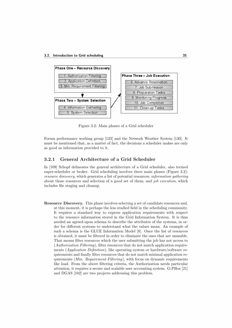
3.2. Introduction to Grid scheduling 35
Figure 3.2: Main phases of a Grid scheduler
Forum performance working group [123] and the Network Weather System [130]. Itmust be mentioned that, as a matter of fact, the decisions a scheduler makes are onlyas good as information provided to it.
3.2.1 General Architecture of a Grid Scheduler
In [109] Schopf delineates the general architecture of a Grid scheduler, also termedsuper-scheduler or broker. Grid scheduling involves three main phases (Figure 3.2):resource discovery, which generates a list of potential resources; information gatheringabout those resources and selection of a good set of them; and job execution, whichincludes file staging and cleanup.
Resource Discovery. This phase involves selecting a set of candidate resources and,at this moment, it is perhaps the less studied field in the scheduling community.It requires a standard way to express application requirements with respectto the resource information stored in the Grid Information System. It is thusneeded an agreed-upon schema to describe the attributes of the systems, in or-der for different systems to understand what the values mean. An example ofsuch a schema is the GLUE Information Model [8]. Once the list of resourcesis obtained, it must be filtered in order to eliminate the ones that are unusable.That means filter resources which the user submitting the job has not access to(Authorization Filtering), filter resources that do not match application require-ments (Application Definition), like operating system or hardware/software re-quirements and finally filter resources that do not match minimal application re-quirements (Min. Requirement Filtering), with focus on dynamic requirementslike load. From the above filtering criteria, the Authorization needs particularattention, it requires a secure and scalable user accounting system. G-PBox [21]and DGAS [102] are two projects addressing this problem.

36 3. Grid scheduling
System Selection. While the previous phase filters out unsuitable resources, thisphase should determine from this large list the best (set of) resource(s) chosento map the application. This selection requires to gather detailed dynamicinformation from resources (Information Gathering), e.g. by accessing localGRIS of Globus middleware, or querying performance prediction systems suchas Network Weather System (NWS) [130]. This information should be used torank resources, and to allow the scheduler to choose the ones that should ensurehigh performance in the execution of the application (System Selection).
Job Execution. The last phase is running the job. This phase can be very complexand can require various intermediary steps:
1. Advance reservation: this is an optional step. Part or all the resourcesneeded for the job can be reserved in advance.
2. Job submission: the job is submitted to the selected resource for execution.
3. Preparation tasks: preliminary operations needed for the execution of thejobs. Can include the retrieval of input files, claiming a reservation, etc.
4. Monitoring progress: it is essential for a user to know where and how theexecution is going on. These information are useful also for the schedulingalgorithm, for example by rescheduling the job if it is not making sufficientprogress.
5. Job completion: notification of the result of the execution.
6. Cleanup tasks: retrieving of output files, removing of temporary data andsettings, and so forth.
While many schedulers have begun to address the needs of a true Grid-level scheduler,none of them currently supports the full range of actions required.
The next section gives on overview of Grid workflows, which have a growing in-terest and have an important impact in scheduling issues. The rest of the chapterbriefly describes some implementations of scheduling systems.
3.3 Grid Workflows
Grid workflows are an emerging research field in the Grid community. Actually thereis an ongoing effort to define a standard meaning of workflow for the Grid. Thissection wants to outline motivations, issues and approaches currently followed.
We said above how Grid is emerging as a service oriented architecture. In particu-lar, the “software as a service” approach results in a componentized view of softwareapplications and workflow can naturally be used as a component composition mech-anism. Traditionally, the main applications of workflow have been in the automationof administrative and production processes, especially within businesses and large or-ganizations. In the late 1990s, Enterprise Application Integration (EAI) emerged asa new application area for workflow. The expansion of workflow towards middleware

3.3. Grid Workflows 37
has since continued, namely within the Web service initiative. The Grid can directlyleverage workflow, both in terms of models and technology.
The users have complex tasks and want to take advantage of the resource-rich en-vironment provided by the Grid to solve their problems subject to a set of constrainssuch as deadlines, cost, quality of the solution. A complex task consists of multi-ple activities. Activities are units of work to be performed by the agents, humans,computers, sensors, and other man-made devices involved in the workflow enactment.A process description, also called a workflow schema, is a structure describing theactivities to be executed and the order of their execution [91]. A workflow has threedimensions:
1. The process: the process dimension refers to the creation and the possible mod-ification of the process description.
2. The case: the case dimension refers to a particular instance of the workflowwhen the attributes required by the process enactment are bound to specificvalues.
3. The resource: the resource dimension refers to discovery and allocation of re-sources needed for the enactment of a case.
Workflow enactment is the process of carrying out the activities prescribed by theprocess description for a particular case.
Two types of workflows can be distinguished: static and dynamic. The processdescription of a static workflow is invariant in time. The process description of adynamic workflow changes during the workflow enactment phase due to circumstancesunforeseen at the process definition time.
There are several distinctions between Grid-based workflows and traditional work-flows encountered in business management, office automation, or production manage-ment [92]:
• The emphasis in a traditional workflow model is placed on the contractual aspectof a transaction. For a Grid-based workflow the enactment of a case is sometimesbased on a ”best-effort model” where the agents involved do their best to attainthe goal state but there is no guarantee of success.
• An important aspect of a transactional model is to maintain a consistent state ofthe system. A Grid is an open system, thus, the state of a Grid is considerablymore difficult to define than the state of a traditional system.
• A traditional workflow consists of a set of well-defined activities that are unlikelyto be altered during the enactment of the workflow. However, the processdescription for a Grid-based workflow may change during the lifetime of a case.After a change, the enactment of a case may continue based on the older processdescription, while under some circumstances it may be based on the newerprocess description. In addition to static workflows we have to support dynamicones.
38 3. Grid scheduling
• The activities of a Grid-based workflow could be long lasting. Some of theactivities supported by the Grid are collaborative in nature and the workflowmanagement should support some form of merging of partial process descrip-tions.
• The individual activities of a Grid workflow may not exhibit the traditionalproperties of transactions. Consider, for example, durability; at any instance oftime before reaching the goal state a workflow may roll back to some previouslyencountered state and continue from there on an entirely different path. Anactivity of a Grid workflow could be either reversible or irreversible. Sometimes,paying a penalty for reversing an activity is more profitable in the long run thancontinuing on a wrong path.
• Resource allocation is a critical and very delicate aspect of the Grid-based work-flow enactment. The Grid provides a resource-rich environment with multipleclasses of resources and many administrative domains; there is a large variabil-ity of resources in each class; resource utilization is bursty in nature. Thus,we need: resource discovery services, support for negotiations among multipleadministrative domains, matching and brokerage services, reservations mecha-nisms, support for dynamic resource allocation, and other sophisticated resourcemanagement mechanisms and services.
• Mobility of various agents involved in the enactment of a case is important forGrid-based workflows. The agents may relocate to the proximity of the siteswhere activities are carried-out to reduce communication costs and latency.
At least four important issues can be identified in order to enable workflows for theGrid:
1. User Environments or Workflow IDE (Integrated Development Environment).
2. Representation and language to express workflow.
3. Translation or compilation.
4. Execution and runtime support.
Actually, the most common Grid workflow can be modelled as simple Task (DirectedAcyclic) Graphs (DAGs), where the order of execution of tasks (modelled as nodes)is determined by dependencies (in turn modelled as directed arcs). Each DAG noderepresents the execution of a component, characterized by a set of attributes such asan estimate of its cost and possible requirements on the target execution platform,while DAG directed edges represent data dependencies between specific applicationcomponents. Data dependencies will be usually constituted by large files written bya component and required for the execution of one or more other components of theapplication.
In the following section we will survey the main approaches to scheduling systems,that considers workflow scheduling, currently followed in the Grid community.
3.4. Grid scheduling systems 39
3.4 Grid scheduling systems
In this section we present a brief description of some Grid scheduling systems thatmanages workflows [136, 10].
3.4.1 Condor DAGMan
Condor [86, 119, 120] is a specialized resource management system (RMS) developedat the University of Wisconsin-Madison for compute-intensive jobs. Like other full-featured batch systems, Condor provides a job queuing mechanism, scheduling policy,priority scheme, resource monitoring, and resource management. Users submit theirserial or parallel jobs to Condor, Condor places them into a queue, chooses whenand where to run the jobs based upon a policy, carefully monitors their progress,and ultimately informs the user upon completion. Condor can be used to manage acluster of dedicated compute nodes (such as a “Beowulf” cluster). In addition, uniquemechanisms enable Condor to effectively harness wasted CPU power from otherwiseidle desktop workstations. Some of the enabling mechanisms of Condor are:
• ClassAds: it is a framework for matching resource requests (e.g. jobs) withresource offers (e.g. machines). It allows jobs and resources to advertise theircharacteristics and requirements.
• Job checkpoint and migration: with particular types of jobs, Condor can trans-parently save the state and subsequently resume the application from the check-point file. This technique also permits a job to migrate from one machine toanother machine (low-penalty preemptive-resume scheduling [72]).
• Remote system calls: it is a mechanism for preserving the local execution en-vironment. By redirecting the I/O, for example, the user do not need to makedata files available on remote machines, even in the absence of a shared filesystem.
Condor-G [48] represents the link between two technologies: Condor and theGlobus toolkit [42] (see 2.6). With Condor-G it is possible to use Condor insidea Grid environment. Condor-G can be used as a reliable submission and job man-agement service for one or more sites, Condor as the fabric management service andfinally the Globus toolkit can be used as the bridge between them.
Another service of Condor is the Directed Acyclic Graph Manager (DAGMan)[120] for executing multiple jobs with dependencies described as DAGs. Each jobis a node in the graph and the edges identify their dependencies. DAGMan doesnot support automatic intermediate data movement, so users have to specify datamovement transfer through pre-processing and post-processing commands associatedwith processing job. The DAGMan meta-scheduler processes the DAG dynamically,by sending to the condor scheduler the jobs as soon as their dependencies are satisfiedand they become ready to execute.
40 3. Grid scheduling
3.4.2 GrADS
The Grid Application Development Software (GrADS) project [11] aims to provideprogramming tools and execution environments for ordinary scientific users to de-velop, execute, and tune applications on the Grid. To achieve this goal they areconducting research in four main areas:
1. collaboration on the design and implementation in prototype form of importantscientific applications for the Grid;
2. design of programming systems and problem-solving environments;
3. design and implementation of schedulers that dynamically match configurableapplications to available resources;
4. design and construction of hardware and software testbeds for experimentation.
In GrADS applications are encapsulated as configurable object programs (COPs). ACOP includes code for the application (e.g. an MPI program), a mapper that de-termines how to map an application’s tasks to a set of resources, and an executableperformance model that estimates the application’s performance on a set of resources.The system relies upon performance contracts that specify the expected performanceof modules as a function of available resources.
The GrADS project has recently included the possibility of scheduling workflowapplications [25]. The implemented workflow scheduling has the objective of minimizethe overall job completion time, or makespan, of the application. The mapping fromthe workflow components to the Grid resources is based on the merging of two models:the model of the Grid resources, determined using Grid services such as the MDS [39]and NWS [130], and the performance model of the application. For each applicationcomponent, the GrADS workflow scheduler ranks each eligible resource, reflectingthe fit between the component and the resource. After ranking the components, thescheduler uses these information to build a performance matrix and, then, it runsheuristics on this matrix in order to optimize the mapping of independent jobs whenseveral DAG nodes become runnable upon the scheduling of their parents in thegraph. Three heuristics have been applied in GrADS; those are Min-Min, Max-Min,and Sufferage heuristics [89].
The estimate of the performance of a workflow component on a machine is thebase for a good workflow schedule. Performance models are obtained at compile time,when the characteristics of the resources on which the components will run are notknown. Therefore, performance models do not aim to predict an exact executiontime, but rather provide an estimate resource usage that can be converted to a roughtime estimate based on architectural parameters. To obtain the component models,they consider both the number of floating point operations executed and the memoryaccess pattern.
3.5. Summary 41
3.4.3 UNICORE
UNICORE plus [125] provides seamless and secure access to distributed resourcesof the German high performance computing centers. UNICORE plus is a follow-on project of UNICORE (Uniform Interface to Computing Resources) [7] that offersa ready-to-run Grid system including client and server software. The original UNI-CORE job model supports jobs that are constructed as a set of directed acyclic graphswith temporal dependencies. Subsequent versions introduced more sophisticated con-trol facilities in the workflow language. They have introduced advanced flow controlssuch as Do-N, Do-Repeat, If-then-else, and Hold-Job. UNICORE plus offers a graph-ical user interface to construct the application workflow and to convert it into anexecutable object. UNICORE also allows users to explicitly specify the transfer func-tion as a task through GUI; it is also able to perform the necessary data movementfunction without user intervention.
3.5 Summary
The growing computational power requirements of grand challenge applications haspromoted the need for linking high-performance computational resources distributedacross multiple organizations. This is fueled by the availability of the Internet, thegrowing performance of the network infrastructure, low cost high-performance ma-chines such as clusters across multiple organizations, and the rise of scientific problemsof multi-organizational interest.
Computational Grids are expected to offer dependable, consistent, pervasive, andinexpensive access to high-end resources irrespective of their physical location andthe location of access points. Due to the use of geographically distributed multiorga-nizational resources, the Grid computing environment needs to dynamically addressissues involved in inter-domain resource usage and should have the following features:site autonomy, heterogeneity, extensibility, allocation/co-allocation, scheduling, andonline control.
A Grid scheduler (or broker) must make resource selection decisions in an environ-ment where it has no control over the local resources, the resources are distributed,and information about the systems is often limited or dated. These interactions arealso closely tied to the functionality of the Grid Information Services. This Gridscheduling approach has three phases: resource discovery, system selection, and jobexecution.
Scientists and engineers are building more and more complex applications to man-age and process large data sets, and execute scientific experiments on distributedresources. Such application scenarios require means for composing and executingcomplex workflows. Grid is emerging as a service oriented architecture. In particu-lar, the “software as a service” approach results in a componentized view of softwareapplications and workflow can naturally be used as a component composition mecha-nism. Two types of workflows can be distinguished: static and dynamic. The processdescription of a static workflow is invariant in time. The process description of a dy-
42 3. Grid scheduling
namic workflow changes during the workflow enactment phase due to circumstancesunforeseen at the process definition time. Actually, the most common Grid workflowcan be modelled as simple Task (Directed Acyclic) Graphs (DAGs), where the orderof execution of tasks (modelled as nodes) is determined by dependencies (in turnmodelled as directed arcs).
In the recent past, several Grid workflow systems have been proposed and devel-oped. Some examples are the Condor DAGman, the GrADS project, the UNICOREproject.
4Literature survey of the DAG
scheduling problem
In this chapter we present background and a brief survey of the most representa-tive DAG scheduling algorithms found in the literature. We first introduce the DAGscheduling problem giving a general description of the problem statement. This is fol-lowed by a discussion about the NP-completeness of variants of the scheduling prob-lem. We describe the DAG model of a parallel program and the computing systemenvironment which executes the application. A lot of (earlier) works make simplifyingassumption like restricted graph structures, no communication among tasks, etc. Wediscuss the difficulties in considering the general problem, in particular in presenceof communication: the concept of granularity of a DAG is defined. In order to intro-duce the description of the most representative scheduling algorithms, we illustratea taxonomy based on the classification of different scheduling environments. Most ofthe algorithms work on homogeneous and heterogeneous systems. However, the het-erogeneity is mostly intended as machine heterogeneity and do not consider networkheterogeneity. This means that a message is transmitted with the same speed on alllinks. This assumption cannot be made in a Grid environment. Some recent workson scheduling parallel applications in heterogeneous systems with a heterogeneousinterconnection network are presented.
4.1 The DAG scheduling problem
The scheduling problem is very important for the effective utilization of distributedcomputer systems. The general scheduling problem can be divided into two cate-gories: independent jobs scheduling and multiple interacting jobs scheduling. In theformer category, independent jobs are to be scheduled among the processors of a dis-tributed computing system to optimize the overall system performance. The lattercategory requires the allocation of multiple interacting tasks (considered like a sin-gle parallel program) without violating precedence constraints in order to minimizethe completion time on the parallel computer system. The scheduling problem canbe addressed in both static as well as dynamic contexts. When the characteristics
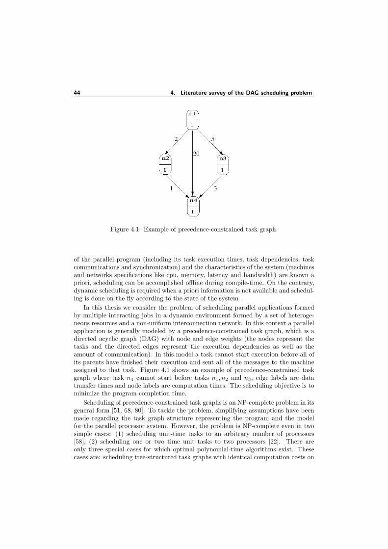
44 4. Literature survey of the DAG scheduling problem
Figure 4.1: Example of precedence-constrained task graph.
of the parallel program (including its task execution times, task dependencies, taskcommunications and synchronization) and the characteristics of the system (machinesand networks specifications like cpu, memory, latency and bandwidth) are known apriori, scheduling can be accomplished offline during compile-time. On the contrary,dynamic scheduling is required when a priori information is not available and schedul-ing is done on-the-fly according to the state of the system.
In this thesis we consider the problem of scheduling parallel applications formedby multiple interacting jobs in a dynamic environment formed by a set of heteroge-neous resources and a non-uniform interconnection network. In this context a parallelapplication is generally modeled by a precedence-constrained task graph, which is adirected acyclic graph (DAG) with node and edge weights (the nodes represent thetasks and the directed edges represent the execution dependencies as well as theamount of communication). In this model a task cannot start execution before all ofits parents have finished their execution and sent all of the messages to the machineassigned to that task. Figure 4.1 shows an example of precedence-constrained taskgraph where task n4 cannot start before tasks n1, n2 and n3, edge labels are datatransfer times and node labels are computation times. The scheduling objective is tominimize the program completion time.
Scheduling of precedence-constrained task graphs is an NP-complete problem in itsgeneral form [51, 68, 80]. To tackle the problem, simplifying assumptions have beenmade regarding the task graph structure representing the program and the modelfor the parallel processor system. However, the problem is NP-complete even in twosimple cases: (1) scheduling unit-time tasks to an arbitrary number of processors[58], (2) scheduling one or two time unit tasks to two processors [22]. There areonly three special cases for which optimal polynomial-time algorithms exist. Thesecases are: scheduling tree-structured task graphs with identical computation costs on
4.1. The DAG scheduling problem 45
an arbitrary number of processors, scheduling arbitrary task graphs with identicalcomputation costs on two processors [60, 111] and, finally, scheduling an interval-ordered DAG with uniform node-weights to an arbitrary number of processors [99]. ADAG is called interval-ordered if every two precedence-related nodes can be mappedto two non-overlapping intervals on the real number line [38]. However, even in thesecases, no communication is assumed among the tasks of the parallel program. It hasbeen shown that scheduling an arbitrary task graph with inter-task communicationonto two processors is NP-complete and scheduling a tree-structured task graph withinter-task communication onto a system with an arbitrary number of processors isalso NP-complete [84].
In order to solve the scheduling problem, three approaches have been suggested:state-space search, dynamic programming and heuristics. The first two techniquesgive optimal solutions under relaxed constraints, but they are not useful since mostof them work under restricted environments and most importantly they lead to anexponential time in the worst case. Heuristics are the usual approach to solve thescheduling problem. They achieve good efficiency, but, on the other side, they usuallycannot generate optimal solutions and there is no guarantee about their performancein general, since the average, worst, and best case performance of these algorithmsare not known.
Most scheduling heuristics algorithms are based on the list scheduling approach.The basic idea in list scheduling is to assign priorities to nodes and examine forscheduling higher priority nodes first, ties are broken using some method specificto each algorithm. There are numerous variations in how the priority are assignedand in maintaining the list of ready nodes, and criteria for selecting a processor toaccommodate a task. We describe later in this chapter (section 4.6) some of thesealgorithms. There are two approaches used in the list scheduling: static and dynamic.In static list scheduling the list of nodes is statically constructed before task allocationbegins, and the sequencing in the list is not modified during the other operations.In dynamic list scheduling priorities are updated after each allocation and the listof ready tasks is consequently rearranged. Dynamic list scheduling algorithms canpotentially generate better schedules (at the cost of increasing the time-complexity), inparticular if they have to operate in a Grid environment, which is extremely dynamic.In a Grid the resources are shared by all the users and the load of the network and ofthe machines change also during application execution. Moreover, the resources cancome and go and the initial static schedule can become completely useless.
In realistic cases, a scheduling algorithm needs to address a number of issues.It should exploit the parallelism by identifying the task graph structure, and takeinto consideration task granularity (amount of computation with respect to commu-nication), arbitrary computation and communication costs. Moreover, in order to beof practical use, a scheduling algorithm should have low complexity and should beeconomical in terms of the number of processors used.
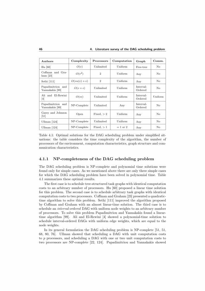
46 4. Literature survey of the DAG scheduling problem
Authors Complexity Processors Computation Graph Comm.
Hu [60] O(v) Unlimited Uniform Free-tree No
Coffman and Gra-ham [23]
O(v2) 2 Uniform Any No
Sethi [111] O(vα(v) + e) 2 Uniform Any No
Papadimitriou andYannakakis [99]
O(v + e) Unlimited Uniform Interval-Ordered
No
Ali and El-Rewini[4]
O(ve) Unlimited Uniform Interval-Ordered
Uniform
Papadimitriou andYannakakis [99]
NP-Complete Unlimited Any Interval-Ordered
No
Garey and Johnson[51]
Open Fixed, > 2 Uniform Any No
Ullman [124] NP-Complete Unlimited Uniform Any No
Ullman [124] NP-Complete Fixed, > 1 = 1 or 2 Any No
Table 4.1: Optimal solutions for the DAG scheduling problem under simplified sit-uations: the table considers the time complexity of the algorithm, the number ofprocessors of the environment, computation characteristics, graph structure and com-munication characteristics.
4.1.1 NP-completeness of the DAG scheduling problem
The DAG scheduling problem is NP-complete and polynomial time solutions werefound only for simple cases. As we mentioned above there are only three simple casesfor which the DAG scheduling problem have been solved in polynomial time. Table4.1 summarizes these optimal results.
The first case is to schedule tree-structured task graphs with identical computationcosts to an arbitrary number of processors. Hu [60] proposed a linear time solutionfor this problem. The second case is to schedule arbitrary task graphs with identicalcomputation costs to two processors. Coffman and Graham [23] presented a quadratic-time algorithm to solve this problem. Sethi [111] improved the algorithm proposedby Coffman and Graham with an almost linear-time solution. The third case is toschedule an interval-ordered DAG with uniform node weights to an arbitrary numberof processors. To solve this problem Papadimitriou and Yannakakis found a linear-time algorithm [99]. Ali and El-Rewini [4] showed a polynomial-time solution toschedule interval-ordered DAGs with uniform edge weights, which are equal to thenode weights.
In its general formulation the DAG scheduling problem is NP-complete [51, 51,68, 80, 76]. Ullman showed that scheduling a DAG with unit computation coststo p processors, and scheduling a DAG with one or two unit computation costs totwo processors are NP-complete [22, 124]. Papadimitriou and Yannakakis showed
4.2. Background 47
that scheduling an interval ordered DAG with arbitrary computation costs to twoprocessors is NP-complete [99] and scheduling a DAG with unit computation coststo p processors, possibly with task-duplication, is also NP-complete [100]. Finally,Garey et al. [50] showed that scheduling an opposing forest with unit computationto p processors is NP-complete.
4.2 Background
A parallel program can be represented by a directed acyclic graph (DAG). A DAG isa tuple G = (V,E) where V = {nj , j = 1..v} is the set of nodes with |V | = v, E isthe set of communication edges and |E| = e. Nodes and edges are labeled as follows:
• the weight ci,j ∈ C is the communication cost incurred along the edge ei,j =(ni, nj) ∈ E, which becomes zero if both nodes are mapped to the same proces-sor;
• the weight τi ∈ T of the node ni ∈ V is the computation cost (or the expectedexecution time) of the task represented by the node ni.
A task is a set of instructions that must be executed sequentially in the same processorwithout preemption. A task cannot start execution before all of its parents havefinished their execution and sent all of the messages to the machine assigned to thattask. Hereafter we use the terms node and task interchangeably. Two tasks are calledindependent if there are no dependence paths between them. The width of a DAGis the size of the maximal set of independent tasks. A node is a source node if ithas no incoming edges and it is an exit node if it has no outgoing edges.
DAG scheduling algorithms found in the literature usually assume as startingpoint a DAG labeled with estimates of computation times and data transfer times. Inpractice we have to distinguish between two types of DAGs: abstract and concrete.The abstract DAG is labelled with relative values, which do not aim to predict anexact execution time, but rather provide an estimated resource usage that can beconverted to a rough time estimate based on architectural parameters. The abstractDAG is obtained at compile-time. The concrete DAG is labelled with time estimatesfor the execution of the tasks and the transfer of the data. An initial static matchingand scheduling phase is necessary in order to obtain the concrete DAG. As noted in[90], the initial mapping can be realized using a static mapping algorithm such asthe baseline [126], genetic-algorithm-based mapper [126] or Levelized Min Time [64].In particular, when we are dealing with a heterogeneous and dynamic environment,time estimates are not known prior to application execution and the initial mappingmust be done at run-time before the execution of the scheduling algorithm. All thealgorithms described in the following sections assume the initial DAG to be concrete.
If we denote with ST (ni) and with FT (ni), respectively, the start and finish-timeof the task ni, then the schedule length can be defined as maxi{FT (ni)}. Theobjective of DAG scheduling is to minimize of the schedule length or makespan
48 4. Literature survey of the DAG scheduling problem
maxi{FT (ni)}, without violating precedence constraints. Just as qualitative defini-tion, a schedule is considered efficient if the scheduled length is short and the numberof processors used is reasonable.
Node and edge weights are usually obtained by estimation once the characteristicsof the environment (cpu, memory, latency, bandwidth, etc.) are known. Estimatesare computed by considering information such as number of floating point operationsand memory access pattern. Obtaining these estimates is actually an active area ofresearch. For example, considering Grid context, we can find the GrADS project[25], where performance models are built at compile time for each task. Performancemodels are an architecture-independent model of the workflow component providingan estimated resource usage that can be converted to a rough time estimate whenarchitectural parameters of the resource will be available.
The DAG scheduling problem is usually identified by the combination of twophases: matching which assigns tasks to machines and scheduling which definesthe execution order of the tasks assigned to each machine. The overall problem ofmatching and scheduling is referred to as mapping.
4.2.1 The computing system
The computing system, which executes the parallel application, is generally assumedto be a network of processing elements (PEs), each of which is composed of a proces-sor and a local memory unit so that the PEs do not share memory and communica-tion relies solely on message-passing. There can be two types of computing system:homogeneous and heterogeneous. A heterogeneous computing system consists of aheterogeneous suite of machines having different speeds or processing capabilities.The machines are connected by a network. The topology of the network may befully-connected or of a particular structure such as a hypercube or a mesh. Althoughmost of the scheduling algorithms that can be found in the literature assume an envi-ronment with heterogeneous processors, usually the communication links are assumedto be homogeneous, i.e., a message is transmitted with the same speed on all links.In contrast, a Grid has both heterogeneous machines and communication links. Thedata communication time between two machines has two components: a fixed mes-sage latency for the first byte to arrive and a per byte message transfer time. Insuch situations, an |M | × |M | communication matrix, where |M | is the number ofmachines, is used to hold these values for the heterogeneous computing (HC) suite.
4.2.2 DAG scheduling preliminaries
As we mentioned above, most of the scheduling algorithms are based on the listscheduling technique. These algorithms assign priorities to the tasks and schedulethem according to a list priority scheme. A node with higher priority is examined forscheduling before a node with lower priority. This technique is based on the repeatedexecution of the following two steps for as long as all the tasks of the DAG are mapped:
1. select the node with higher priority;
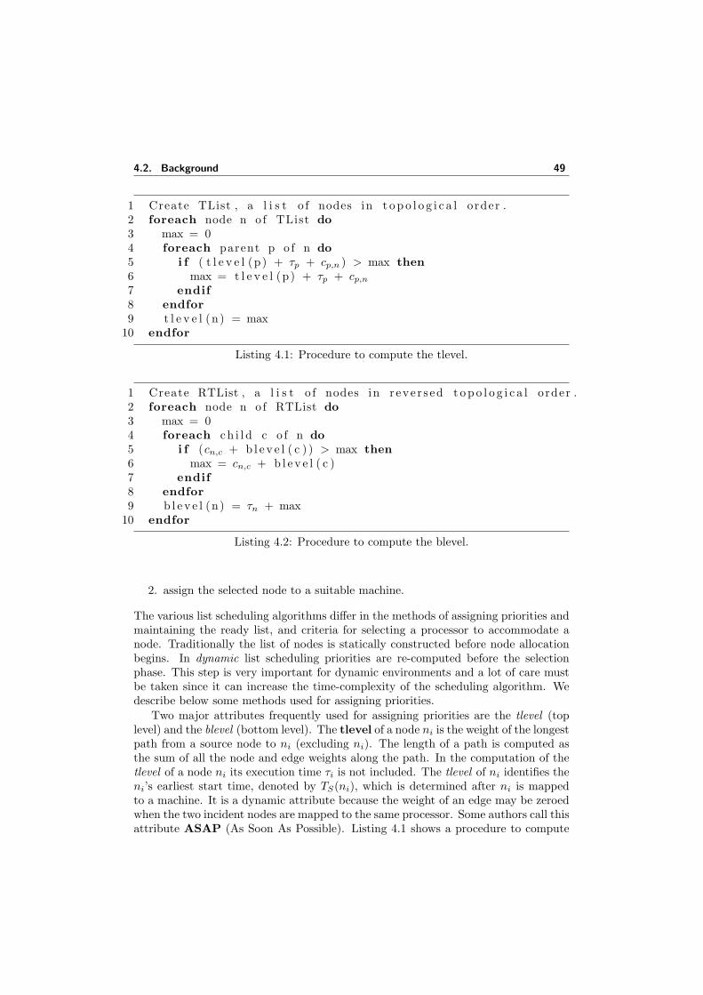
4.2. Background 49
1 Create TList , a l i s t o f nodes in t o p o l o g i c a l order .2 foreach node n o f TList do3 max = 04 foreach parent p o f n do5 i f ( t l e v e l (p) + τp + cp,n ) > max then6 max = t l e v e l (p) + τp + cp,n
7 endif8 endfor9 t l e v e l (n) = max
10 endfor
Listing 4.1: Procedure to compute the tlevel.
1 Create RTList , a l i s t o f nodes in r eve r s ed t o p o l o g i c a l order .2 foreach node n o f RTList do3 max = 04 foreach ch i l d c o f n do5 i f (cn,c + b l e v e l ( c ) ) > max then6 max = cn,c + b l e v e l ( c )7 endif8 endfor9 b l e v e l (n) = τn + max
10 endfor
Listing 4.2: Procedure to compute the blevel.
2. assign the selected node to a suitable machine.
The various list scheduling algorithms differ in the methods of assigning priorities andmaintaining the ready list, and criteria for selecting a processor to accommodate anode. Traditionally the list of nodes is statically constructed before node allocationbegins. In dynamic list scheduling priorities are re-computed before the selectionphase. This step is very important for dynamic environments and a lot of care mustbe taken since it can increase the time-complexity of the scheduling algorithm. Wedescribe below some methods used for assigning priorities.
Two major attributes frequently used for assigning priorities are the tlevel (toplevel) and the blevel (bottom level). The tlevel of a node ni is the weight of the longestpath from a source node to ni (excluding ni). The length of a path is computed asthe sum of all the node and edge weights along the path. In the computation of thetlevel of a node ni its execution time τi is not included. The tlevel of ni identifies theni’s earliest start time, denoted by TS(ni), which is determined after ni is mappedto a machine. It is a dynamic attribute because the weight of an edge may be zeroedwhen the two incident nodes are mapped to the same processor. Some authors call thisattribute ASAP (As Soon As Possible). Listing 4.1 shows a procedure to compute
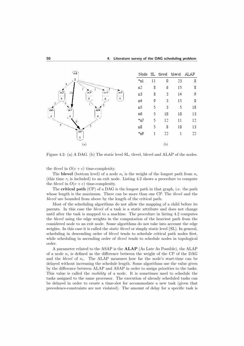
50 4. Literature survey of the DAG scheduling problem
(a) (b)
Figure 4.2: (a) A DAG. (b) The static level SL, tlevel, blevel and ALAP of the nodes.
the tlevel in O(v + e) time-complexity.The blevel (bottom level) of a node ni is the weight of the longest path from ni
(this time τi is included) to an exit node. Listing 4.2 shows a procedure to computethe blevel in O(v + e) time-complexity.
The critical path (CP) of a DAG is the longest path in that graph, i.e. the pathwhose length is the maximum. There can be more than one CP. The tlevel and theblevel are bounded from above by the length of the critical path.
Most of the scheduling algorithms do not allow the mapping of a child before itsparents. In this case the blevel of a task is a static attribute and does not changeuntil after the task is mapped to a machine. The procedure in listing 4.2 computesthe blevel using the edge weights in the computation of the heaviest path from theconsidered node to an exit node. Some algorithms do not take into account the edgeweights. In this case it is called the static blevel or simply static level (SL). In general,scheduling in descending order of blevel tends to schedule critical path nodes first,while scheduling in ascending order of tlevel tends to schedule nodes in topologicalorder.
A parameter related to the ASAP is the ALAP (As Late As Possible), the ALAPof a node ni is defined as the difference between the weight of the CP of the DAGand the blevel of ni. The ALAP measures how far the node’s start-time can bedelayed without increasing the schedule length. Some algorithms use the value givenby the difference between ALAP and ASAP in order to assign priorities to the tasks.This value is called the mobility of a node. It is sometimes used to schedule thetasks assigned to the same processor. The execution of already scheduled tasks canbe delayed in order to create a time-slot for accommodate a new task (given thatprecedence-constraints are not violated). The amount of delay for a specific task is

4.2. Background 51
(a) (b) (c)
Figure 4.3: (a) A DAG. (b) A Gantt chart for a schedule. (c) A scheduled DAG
given by its mobility attribute.In figure 4.2 we can see an example of DAG where nodes n1, n7 and n9 belong to
the critical path. In this case the critical path is unique. The edges of the criticalpath are shown with thick arrows. If we change, for example, the weight of the edge(n8, n9) from 5 to 10, then also the nodes n1, n4, n8 and n9 lie on a critical path, twoCPs of weight 23.
Figure 4.3(a) shows an example of weighted DAG, figure 4.3(b) a Gantt chart fora possible schedule of that DAG and figure 4.3(c) the corresponding scheduled DAG.The Gantt chart defines the processor assignment, the starting and the completiontimes for each task. A scheduled DAG is a DAG with included precedence con-straints given an assigned schedule. In figure 4.3(c) the two clusters are circled and theedges (drawn with thick lines) corresponding to task execution ordering informationfor tasks assigned to the same processor are: (n3, n4) and (n5, n3).
A cluster with only one task is called a unit cluster. Clusters can be dividedinto two groups: linear and nonlinear. A cluster is called nonlinear if there areat least two independent tasks in the same cluster, otherwise it is called linear. Forexample, in figure 4.3(c) there are two clusters: one is a linear cluster and contains thenodes n1 and n2, the other is nonlinear because nodes n3, n4 and n5 are independentin the original DAG (figure 4.3(a)). Since a schedule imposes an ordering of tasksin nonlinear clusters, the nonlinear clusters of a DAG can be thought of as linearclusters in the scheduled DAG if execution orders between independent tasks arecounted as edges. It is important to note that liner clusters preserve the parallelismof the DAG while nonlinear clusters reduces parallelism by sequentializing paralleltasks. The core point of the DAG scheduling problem is to find the best tradeoff
52 4. Literature survey of the DAG scheduling problem
Symbol DefinitionV The set of nodes (tasks) in the DAG.E The set of edges (communication links) in the DAG.ni Node (task) of the DAG (ni ∈ V ).
ei,j or (ni, nj) Edge from task ni to task nj (ei,j∈E).τi The execution time of node (task) ni.ci,j The communication time between the tasks.
CCR Communication to computation ratio.tlevel(ni) Top level of task ni (earliest start time).blevel(ni) Bottom level of task ni.
CP Critical Path (longest path in the DAG).DS Dominant Sequence (critical path of the scheduled DAG).
ASAP (ni) As Soon As Possible (same as tlevel(ni) or earliest start time).ALAP (ni) As Late As Possible.
Table 4.2: Some notations and their definitions
between sequentialization and parallelization. A discussion about this issue can befound in [54]. In section 4.2.3 we briefly summarize that work.
A task is free if it has no predecessors or if all its predecessors have been examinedand mapped to a resource. A task is partially free if some of its predecessors havebeen examined and mapped to a resource.
A ready task is a task that can immediately start its execution because all thedata it is waiting for (from its parents) are available on the assigned machine. A taskis not ready if it is still waiting for data. A ready task is also a free task, but a freetask can be ready or not.
The Dominant Sequence (DS) is the critical path of the scheduled DAG and itsweight is called the parallel time. The following formula can be used to determinethe parallel time of a scheduled DAG:
PT = maxni∈V
{tlevel(ni) + blevel(ni)}.
Table 4.2 summarizes some notations and their definitions.
4.2.3 Clustering of a DAG: communication and granularity
In presence of communication the scheduling problem is much harder [134, 54], mainlybecause the edge weights are no longer deterministic before the processor assignmentshave been done. Communication is zero when two tasks are mapped in the same pro-cessor, and nonzero when they are mapped in two different processors. Since thescheduling objective is the minimization of the makespan, assigning different tasksto the same processors can lead to a better schedule. The process of grouping dif-ferent tasks is called clustering. Every task in a cluster must execute in the same
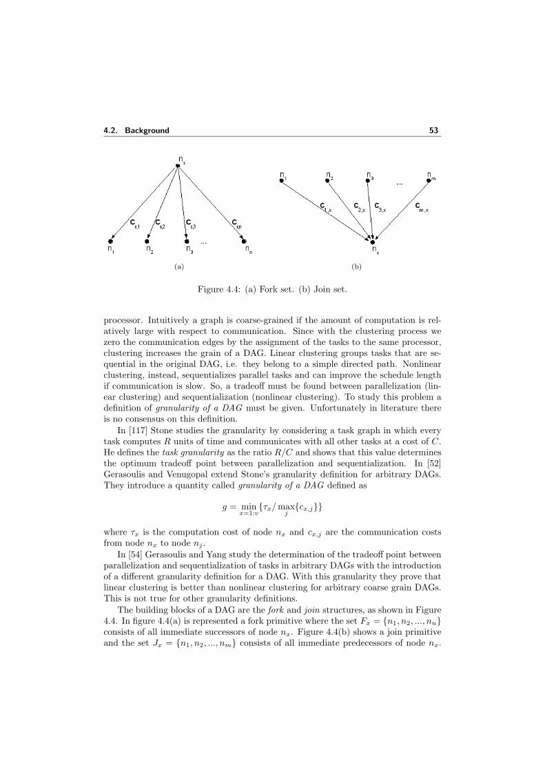
4.2. Background 53
(a) (b)
Figure 4.4: (a) Fork set. (b) Join set.
processor. Intuitively a graph is coarse-grained if the amount of computation is rel-atively large with respect to communication. Since with the clustering process wezero the communication edges by the assignment of the tasks to the same processor,clustering increases the grain of a DAG. Linear clustering groups tasks that are se-quential in the original DAG, i.e. they belong to a simple directed path. Nonlinearclustering, instead, sequentializes parallel tasks and can improve the schedule lengthif communication is slow. So, a tradeoff must be found between parallelization (lin-ear clustering) and sequentialization (nonlinear clustering). To study this problem adefinition of granularity of a DAG must be given. Unfortunately in literature thereis no consensus on this definition.
In [117] Stone studies the granularity by considering a task graph in which everytask computes R units of time and communicates with all other tasks at a cost of C.He defines the task granularity as the ratio R/C and shows that this value determinesthe optimum tradeoff point between parallelization and sequentialization. In [52]Gerasoulis and Venugopal extend Stone’s granularity definition for arbitrary DAGs.They introduce a quantity called granularity of a DAG defined as
g = minx=1:v
{τx/ maxj{cx,j}}
where τx is the computation cost of node nx and cx,j are the communication costsfrom node nx to node nj .
In [54] Gerasoulis and Yang study the determination of the tradeoff point betweenparallelization and sequentialization of tasks in arbitrary DAGs with the introductionof a different granularity definition for a DAG. With this granularity they prove thatlinear clustering is better than nonlinear clustering for arbitrary coarse grain DAGs.This is not true for other granularity definitions.
The building blocks of a DAG are the fork and join structures, as shown in Figure4.4. In figure 4.4(a) is represented a fork primitive where the set Fx = {n1, n2, ..., nn}consists of all immediate successors of node nx. Figure 4.4(b) shows a join primitiveand the set Jx = {n1, n2, ..., nm} consists of all immediate predecessors of node nx.
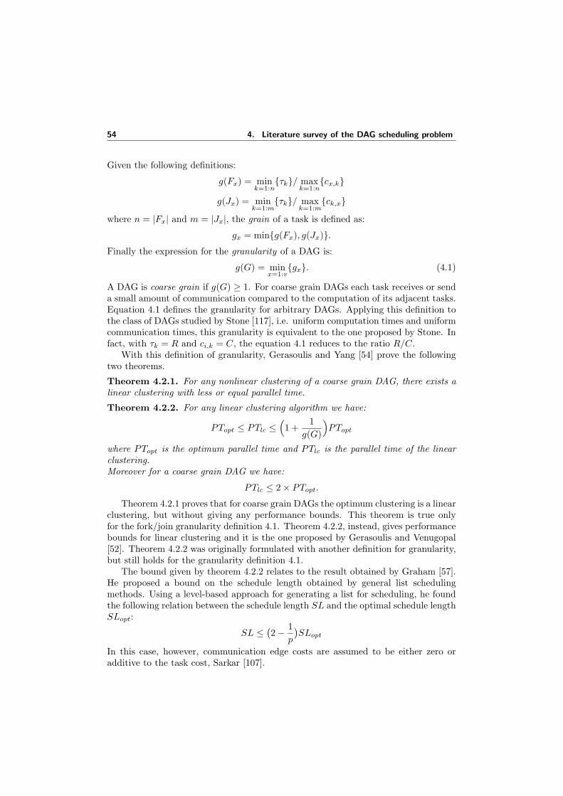
54 4. Literature survey of the DAG scheduling problem
Given the following definitions:
g(Fx) = mink=1:n
{τk}/ maxk=1:n
{cx,k}
g(Jx) = mink=1:m
{τk}/ maxk=1:m
{ck,x}
where n = |Fx| and m = |Jx|, the grain of a task is defined as:
gx = min{g(Fx), g(Jx)}.
Finally the expression for the granularity of a DAG is:
g(G) = minx=1:v
{gx}. (4.1)
A DAG is coarse grain if g(G) ≥ 1. For coarse grain DAGs each task receives or senda small amount of communication compared to the computation of its adjacent tasks.Equation 4.1 defines the granularity for arbitrary DAGs. Applying this definition tothe class of DAGs studied by Stone [117], i.e. uniform computation times and uniformcommunication times, this granularity is equivalent to the one proposed by Stone. Infact, with τk = R and ci,k = C, the equation 4.1 reduces to the ratio R/C.
With this definition of granularity, Gerasoulis and Yang [54] prove the followingtwo theorems.
Theorem 4.2.1. For any nonlinear clustering of a coarse grain DAG, there exists alinear clustering with less or equal parallel time.
Theorem 4.2.2. For any linear clustering algorithm we have:
PTopt ≤ PTlc ≤(1 +
1g(G)
)PTopt
where PTopt is the optimum parallel time and PTlc is the parallel time of the linearclustering.Moreover for a coarse grain DAG we have:
PTlc ≤ 2× PTopt.
Theorem 4.2.1 proves that for coarse grain DAGs the optimum clustering is a linearclustering, but without giving any performance bounds. This theorem is true onlyfor the fork/join granularity definition 4.1. Theorem 4.2.2, instead, gives performancebounds for linear clustering and it is the one proposed by Gerasoulis and Venugopal[52]. Theorem 4.2.2 was originally formulated with another definition for granularity,but still holds for the granularity definition 4.1.
The bound given by theorem 4.2.2 relates to the result obtained by Graham [57].He proposed a bound on the schedule length obtained by general list schedulingmethods. Using a level-based approach for generating a list for scheduling, he foundthe following relation between the schedule length SL and the optimal schedule lengthSLopt:
SL ≤(2− 1
p
)SLopt
In this case, however, communication edge costs are assumed to be either zero oradditive to the task cost, Sarkar [107].
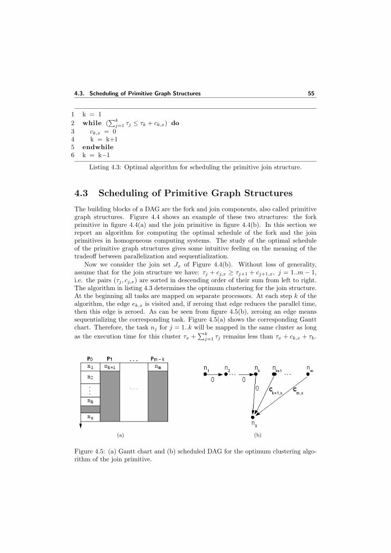
4.3. Scheduling of Primitive Graph Structures 55
1 k = 12 while (
∑kj=1 τj ≤ τk + ck,x) do
3 ck,x = 04 k = k+15 endwhile6 k = k−1
Listing 4.3: Optimal algorithm for scheduling the primitive join structure.
4.3 Scheduling of Primitive Graph Structures
The building blocks of a DAG are the fork and join components, also called primitivegraph structures. Figure 4.4 shows an example of these two structures: the forkprimitive in figure 4.4(a) and the join primitive in figure 4.4(b). In this section wereport an algorithm for computing the optimal schedule of the fork and the joinprimitives in homogeneous computing systems. The study of the optimal scheduleof the primitive graph structures gives some intuitive feeling on the meaning of thetradeoff between parallelization and sequentialization.
Now we consider the join set Jx of Figure 4.4(b). Without loss of generality,assume that for the join structure we have: τj + cj,x ≥ τj+1 + cj+1,x, j = 1..m − 1,i.e. the pairs (τj , cj,x) are sorted in descending order of their sum from left to right.The algorithm in listing 4.3 determines the optimum clustering for the join structure.At the beginning all tasks are mapped on separate processors. At each step k of thealgorithm, the edge ek,x is visited and, if zeroing that edge reduces the parallel time,then this edge is zeroed. As can be seen from figure 4.5(b), zeroing an edge meanssequentializing the corresponding task. Figure 4.5(a) shows the corresponding Ganttchart. Therefore, the task nj for j = 1..k will be mapped in the same cluster as longas the execution time for this cluster τx +
∑kj=1 τj remains less than τx + ck,x + τk.
(a) (b)
Figure 4.5: (a) Gantt chart and (b) scheduled DAG for the optimum clustering algo-rithm of the join primitive.
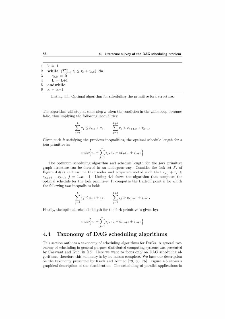
56 4. Literature survey of the DAG scheduling problem
1 k = 12 while (
∑kj=1 τj ≤ τk + cx,k) do
3 cx,k = 04 k = k+15 endwhile6 k = k−1
Listing 4.4: Optimal algorithm for scheduling the primitive fork structure.
The algorithm will stop at some step k when the condition in the while loop becomesfalse, thus implying the following inequalities:
k∑j=1
τj ≤ ck,x + τk,
k+1∑j=1
τj > ck+1,x + τk+1.
Given such k satisfying the previous inequalities, the optimal schedule length for ajoin primitive is:
max{
τx +k∑
j=1
τj , τx + ck+1,x + τk+1
}The optimum scheduling algorithm and schedule length for the fork primitive
graph structure can be derived in an analogous way. Consider the fork set Fx ofFigure 4.4(a) and assume that nodes and edges are sorted such that cx,j + τj ≥cx,j+1 + τj+1, j = 1..n − 1. Listing 4.4 shows the algorithm that computes theoptimal schedule for the fork primitive. It computes the tradeoff point k for whichthe following two inequalities hold:
k∑j=1
τj ≤ cx,k + τk,
k+1∑j=1
τj > cx,k+1 + τk+1.
Finally, the optimal schedule length for the fork primitive is given by:
max{
τx +k∑
j=1
τj , τx + cx,k+1 + τk+1
}4.4 Taxonomy of DAG scheduling algorithms
This section outlines a taxonomy of scheduling algorithms for DAGs. A general tax-onomy of scheduling in general-purpose distributed computing systems was presentedby Casavant and Kuhl in [18]. Here we want to focus only on DAG scheduling al-gorithms, therefore this summary is by no means complete. We base our descriptionon the taxonomy presented by Kwok and Ahmad [79, 80, 76]. Figure 4.6 shows agraphical description of the classification. The scheduling of parallel applications in
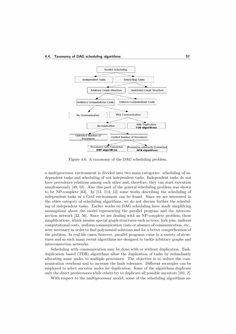
4.4. Taxonomy of DAG scheduling algorithms 57
Figure 4.6: A taxonomy of the DAG scheduling problem.
a multiprocessor environment is divided into two main categories: scheduling of in-dependent tasks and scheduling of not independent tasks. Independent tasks do nothave precedence relations among each other and, therefore, they can start executionsimultaneously [49, 55]. Also this part of the general scheduling problem was shownto be NP-complete [63]. In [13, 114, 12] some works describing the scheduling ofindependent tasks in a Grid environment can be found. Since we are interested inthe other category of scheduling algorithms, we do not discuss further the schedul-ing of independent tasks. Earlier works on DAG scheduling have made simplifyingassumptions about the model representing the parallel program and the intercon-nection network [22, 56]. Since we are dealing with an NP-complete problem, thesesimplifications, which assume special graph structures such as trees, fork-join, uniformcomputational costs, uniform communication costs or absence of communication, etc.,were necessary in order to find polynomial solutions and for a better comprehension ofthe problem. In real life cases, however, parallel programs come in a variety of struc-tures and as such many recent algorithms are designed to tackle arbitrary graphs andinterconnection networks.
Scheduling with communication may be done with or without duplication. Task-duplication based (TDB) algorithms allow the duplication of tasks by redundantlyallocating some nodes to multiple processors. The objective is to reduce the com-munication overhead and to increase the fault tolerance. Different strategies can beemployed to select ancestor nodes for duplication. Some of the algorithms duplicateonly the direct predecessors while others try to duplicate all possible ancestors [101, 2].
With respect to the multiprocessor model, some of the scheduling algorithms as-
58 4. Literature survey of the DAG scheduling problem
sume an unlimited availability of processors, while other scheduling algorithms as-sume an environment with a limited number of processors. The algorithms belong-ing to the former class are called UNC (Unbounded Number of Clusters) schedul-ing algorithms [67, 74, 78, 107, 131, 135, 76, 74], and the ones belonging to thelatter class are called BNP (Bounded Number of Processors) scheduling algorithms[116, 98, 97, 93, 75, 66, 9, 1, 76, 74]. In both UNC and BNP the network is assumedto be fully-connected and no attention is paid to link contention or routing strategiesused for communication. The technique employed by the UNC algorithms is alsocalled clustering [53]. When the algorithm starts, each node is considered a clusteritself. In the subsequent steps, two clusters are merged if the merging reduces thecompletion time. This merging procedure continues until no cluster can be merged.One of the motivations behind the UNC algorithms is that they can take advantageof using more processors to further reduce the schedule length. However, the clus-ters generated by the UNC may need a post-processing step for mapping the clustersonto the processors because the number of processors available may be less than thenumber of clusters.
A few algorithms have been designed to take into account the most general modelin which the system is assumed to consist of an arbitrary network topology, whoselinks are not contention-free. These algorithms are called APN (arbitrary processornetwork) and in addition to scheduling tasks they also schedule messages on thenetwork communication links [3, 127, 115, 110, 103, 94, 73, 69, 62, 35, 32, 77].
4.5 Properties of list scheduling
Since the scheduling problem is NP-complete, considerable attention has been paid onthe performance analysis of the heuristics used to solve this problem, e.g. Sarkar [107],El-Rewini and Lewis [35], Kim and Browne [67], Wu and Gajski [132], Consrad etal. [24], Darte [31], Yang and Gerasoulis [134] and many others. At an early stage ofresearch the scheduling problem was simplified by assuming that communication costis zero. In this context, Graham [57] proved that any list scheduling heuristic is within50% of the optimum. Adam, Chandy and Dickson [1] demonstrated experimentallythat the critical path (CP) list scheduling heuristic is within 5% of the optimumin 90% of the times. If communication is considered then list scheduling no longerprovides the above mentioned performance characteristics.
In [134] Yang and Gerasoulis identify important properties of list scheduling heuris-tics. First they consider the case of list scheduling without communication and givea bound for the CP heuristic. We briefly summarize their result.
Consider the list scheduling as a sequence of merging operations. Initially all tasksare assigned to a unit cluster. At each step the selected task is left in its own clusteror merged to another cluster. Assume that PT i is the parallel time at step i, thenthe merging sequence produces a sequence of parallel times PT 0, PT 1, ..., PTn. Thismeans that, after the last step n, the parallel time is: PT = PTn.
Definition 4.5.1. Let PT iopt be the optimal parallel time at step i, which is the
solution of min{PT i, PT i−1} where the minimum is taken over all possible choices of
4.6. DAG scheduling algorithms 59
free tasks at step i. Then a heuristic is called δ−opt if maxi{PT i−PT iopt} ≤ δ where
δ is a given constant. If δ = 0 then the δ − opt heuristic is called a local optimum.
They can prove the following theorem which gives an upper bound for δ for theCP heuristic.
Theorem 4.5.1. The CP heuristic is δ − opt with δ ≤ ∆T = maxni,nj∈V |τi − τj |.
The important question is if local optimality implies near-optimality. It is verydifficult to prove this result theoretically. Anyway, we do know that the CP heuristicis near optimal [1]. As a consequence of theorem 4.5.1 there is the following corollary,which proves that the CP heuristic is also locally optimal.
Corollary 4.5.1. CP scheduling is locally optimal for DAGs with equal weights.
In general, of course, local optimality does not imply optimality but a near optimalperformance of heuristics that possess this property can be expected.
The scheduling problem is much harder if communication is considered. Yangand Gerasoulis extended their analysis in order to see what type of results can beobtained in the more interesting case of the list scheduling with communication. Inthis case, if a free, but not ready, task is scheduled it must wait for the data toarrive before it can start its execution and an idle gap is created in the schedule. Onthe other hand, if a ready task is chosen for scheduling then it can start its executionimmediately. Therefore, there are two choices for list scheduling: Free List Scheduling(FLS) and Ready List Scheduling. In FLS the highest priority free task is selected formapping, while in RLS the highest priority ready task is selected for mapping. Yangand Gerasoulis extended the δ − opt analysis to the ready list scheduling. RLS usesthe CP heuristic, i.e. the ready tasks with highest priority are selected for mapping.Now the δ − opt definition is slightly different than the one given for list schedulingwithout communication. The local optimum parallel time PT i
opt is derived over allpossible schedules of ready tasks for a selected processor. Given this definition, thefollowing theorem is true.
Theorem 4.5.2. The RCP heuristic is δ − opt with δ ≤ ∆T = maxnj ,ni∈V |τj − τi|.
4.6 DAG scheduling algorithms
In this section we survey some of the DAG scheduling algorithms that can be foundin the literature. We start with earlier optimal algorithms which assume a restrictedDAG model and/or a restricted processor network model, e.g. unit computationweights and no communication. These are the Hu’s algorithm [60] to schedule tree-structured task graphs with identical computation cost to an arbitrary number ofprocessors, the Coffman and Graham [23] algorithm to schedule arbitrary task graphswith identical computation costs to two processors and the Papadimitriou and Yan-nakakis [99] algorithm to schedule an interval-ordered DAG with uniform node weightsto an arbitrary number of processors.
60 4. Literature survey of the DAG scheduling problem
We continue with the description of algorithms that were designed for homo-geneous systems (Sarkar, HLFET, ETF, ISH, FLB, DSC, CASS-II, DCP, MCP andMD). Almost all the algorithms found in the literature work on homogeneous systems.Although the purpose of this thesis is to consider a heterogeneous and dynamic envi-ronment, studying these algorithms is very useful. The heuristics that they define canbe used also in heterogeneous systems, at the cost of increasing the time-complexityof the algorithm.
We conclude with the Hybrid Remapper, an algorithm designed to work in het-erogeneous systems.
4.6.1 Polynomial-time algorithm for Tree-Structured DAGs
This algorithm was proposed by Hu [60]. It is a linear time algorithm that assumes thefollowing simplifications: the graph is an in-tree structured DAG, unit computations,without communication and a limited number of processors equal to p. Rememberthat an in-tree is an oriented tree in which a single vertex is reachable from every otherone. Each node ni is labeled with αi, where αi = xi + 1 and xi is the length of thepath from ni to the exit node in the DAG. Since there is no communication and unitcomputational labels, the length xi is the number of edges in the path. The algorithmconstructs an optimal schedule for p processors by visiting the tree-structured graphin the following steps:
1. Schedule the first p (or fewer) nodes with the highest numbered label to theprocessors, i.e. at the beginning the algorithm schedules, at least, all the entrynodes of the DAG.
2. Remove the p scheduled tasks from the DAG and consider all the nodes withoutpredecessors as entry nodes.
3. Repeat steps (1) and (2) until all nodes are scheduled.
In [60] Hu proves the optimality of the algorithm under the stated constraints.
4.6.2 Arbitrary graphs for a two-processor system
Coffman and Graham [23] proposed an algorithm for generating optimal schedules incase of arbitrary structured graphs with unit computation costs, no communicationand a system with two processors. The first step of the algorithm is to assign labels(with increasing values) to the nodes. The graph is visited bottom-up in a way thatconsiders as candidates for the assignment of the next label all the nodes whosesuccessors have already been assigned a label. When this step is complete, the nodesare ordered by decreasing label numbers . The optimal schedule is computed bymapping ready tasks to idle processors. The algorithm is summarized in the followingsteps:
1. Choose one exit node and assign to it the label 1.
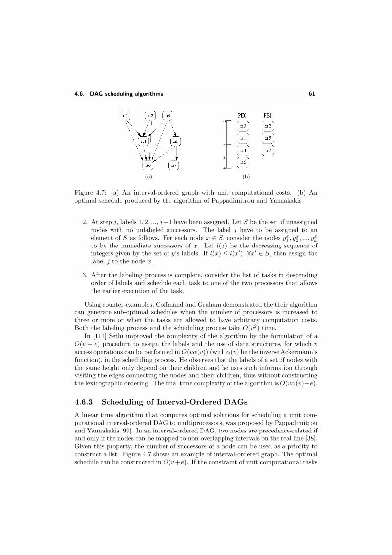
4.6. DAG scheduling algorithms 61
(a) (b)
Figure 4.7: (a) An interval-ordered graph with unit computational costs. (b) Anoptimal schedule produced by the algorithm of Pappadimitrou and Yannakakis
2. At step j, labels 1, 2, ..., j−1 have been assigned. Let S be the set of unassignednodes with no unlabeled successors. The label j have to be assigned to anelement of S as follows. For each node x ∈ S, consider the nodes yx
1 , yx2 , ..., yx
k
to be the immediate successors of x. Let l(x) be the decreasing sequence ofintegers given by the set of y’s labels. If l(x) ≤ l(x′), ∀x′ ∈ S, then assign thelabel j to the node x.
3. After the labeling process is complete, consider the list of tasks in descendingorder of labels and schedule each task to one of the two processors that allowsthe earlier execution of the task.
Using counter-examples, Coffmand and Graham demonstrated the their algorithmcan generate sub-optimal schedules when the number of processors is increased tothree or more or when the tasks are allowed to have arbitrary computation costs.Both the labeling process and the scheduling process take O(v2) time.
In [111] Sethi improved the complexity of the algorithm by the formulation of aO(v + e) procedure to assign the labels and the use of data structures, for which vaccess operations can be performed in O(vα(v)) (with α(v) be the inverse Ackermann’sfunction), in the scheduling process. He observes that the labels of a set of nodes withthe same height only depend on their children and he uses such information throughvisiting the edges connecting the nodes and their children, thus without constructingthe lexicographic ordering. The final time complexity of the algorithm is O(vα(v)+e).
4.6.3 Scheduling of Interval-Ordered DAGs
A linear time algorithm that computes optimal solutions for scheduling a unit com-putational interval-ordered DAG to multiprocessors, was proposed by Pappadimitrouand Yannakakis [99]. In an interval-ordered DAG, two nodes are precedence-related ifand only if the nodes can be mapped to non-overlapping intervals on the real line [38].Given this property, the number of successors of a node can be used as a priority toconstruct a list. Figure 4.7 shows an example of interval-ordered graph. The optimalschedule can be constructed in O(v+e). If the constraint of unit computational tasks
62 4. Literature survey of the DAG scheduling problem
is removed (allowing the tasks to have arbitrary computational weights), the problembecomes NP-complete.
A linear time algorithm to schedule interval-ordered graphs with unit computa-tional costs and unit edge weights was proposed by Ali and El-Rewini [4].
4.6.4 Sarkar’s algorithm
The first clustering algorithm that we consider is the Sarkar’s algorithm [107], that isnot a list scheduling algorithm. Initially it sorts the edges of the DAG in descendingorder of weights. Then at each clustering step the edges are visited in the sorted listorder and zeroed if the parallel time does not increase. The computation of the paralleltime must be done at each clustering step topologically traversing the scheduled DAG.Since there are e such traversals, the complexity is O(e(v + e)) (which dominates theO(e log e) time necessary to sort the edges).
Gerasoulis and Yang [54] noted that imposing the linearity constraint the com-plexity reduces from O(e(v + e)) to O(e log e). At each step the edges that will createnonlinear clusters, if they are zeroed, do not have to be visited. The linearity con-straint ensures that the parallel time at each zeroing step does not increase and itmust not be computed. Therefore, the cost for sorting the edges now dominates thetime complexity of the algorithm. It is a BNP algorithm.
4.6.5 The HLFET algorithm
The HLFET (Highest Level First with Estimated Times) [1] is a list scheduling algo-rithm. It first computes the static blevel for each node and then makes a ready listin descending order of static blevel (ties are broken randomly). Then it repeatedlyschedules the first node in the ready list to a processor that allows the earliest starttime and updates the list with the new ready nodes. It is a BNP algorithm withO(v2) time complexity.
4.6.6 The ETF algorithm
In ETF (Earliest Time First) [61, 105] the main idea is to keep the processor busy,and in this respect being close to a load balancing scheme. At each scheduling step,the priorities for ready unmapped tasks are computed. The task priority is the earli-est start time, which is determined by tentatively mapping the given task to all theprocessors. The selected task is the one with the lowest priority and the selectedprocessor is the one corresponding to this priority. Ties are broken considering stat-ically computed priorities. The time complexity of the algorithm is O(v2p). This isnot a critical path based heuristic and the algorithm does not always map the mostimportant ready task first. Therefore, it may not be able to reduce the partial sched-ule length at every scheduling step. It is a BNP algorithm, since the earliest starttime of a node is computed by examining the start-time of a node on all processorsexhaustively.
4.6. DAG scheduling algorithms 63
4.6.7 The ISH algorithm
The ISH (Insertion Scheduling Heuristic) algorithm [71, 80] tries to fill, as much aspossible, the idle time slots of the processors. It selects ready nodes giving priority tothe ones with higher blevel value (the blevels of the nodes are computed statically atthe beginning of the algorithm). The selected node is assigned to the processor thatallows the earliest execution, using the non-insertion algorithm (the task is scheduledto the processor using a FIFO queue). If the scheduling of this node causes an idletime slot, then the algorithm schedules as many nodes as possible into this idle timeslot, providing that these nodes cannot be scheduled earlier on other processors. Thenit selects a new ready node and repeats all these steps. The time complexity of theISH algorithm is O(v2). It is a BNP algorithm.
4.6.8 The FLB algorithm
The FLB (Fast Load Balancing) algorithm [104] is an improvement of the ETF al-gorithm. It uses the same task selection criteria but the preferred task is identifiedin O(log p) instead of O(wp), where w is the width of the DAG and p the numberof processors. The width of a DAG is the maximum number of independent tasks.Although essentially similar, there is a small difference in the task selection scheme.Throughout the scheduling process it may happen that several ready tasks can startat the same earliest time. ETF and FLB have different criteria to break this tie. Itis a BNP algorithm.
4.6.9 The DSC algorithm
The Sarkar’s algorithm described above, zeroes the highest communication edge. Theedge, however, might not be in a DS that determines the parallel time and as aresult the parallel time might not be reduced at all. The main idea behind the DSC(Dominant Sequence Clustering) algorithm is to perform a sequence of edge zeroingsteps with the goal of reducing a DS at each step [135].
The initial step assumes that each node is mapped in a unit cluster, then thealgorithm tries to merge appropriate clusters by zeroing the edge which connectsthem. During the initialization step the blevel is computed for each node and thetlevel is computed for each free node. Two lists are initialized: a free task list (FL)and a partially free task list (PFL). The free task list is ordered in descending orderconsidering this priority definition:
PRIO(nx) = tlevel(nx) + blevel(nx).
Hence, a DS node can be identified as the one with the highest priority. The tlevel ofa partially free task is defined as:
ptlevel(ny) = maxnj∈PRED(ny)∩EG
{tlevel(nj) + τj + cj,y}
64 4. Literature survey of the DAG scheduling problem
where EG is the set of examined nodes. The priority for the nodes in the partiallyfree task list can be defined as:
pPRIO(ny) = ptlevel(ny) + blevel(ny).
The priority of a partially free node ny is computed considering only the examinedparents of ny. The subsequent steps of the algorithm are briefly described below:
1. Initialization:
• Add all free entry nodes to FL.
• Compute blevel for each node.
• Set tlevel = 0 for each free node.
2. nx = head(FL) and ny = head(PFL).
3. If PRIO(nx) ≥ pPRIO(ny) then minimize tlevel(nx) else minimize tlevel(nx)under constraint DSRW.
4. Update the priorities of nx’s successors.
5. Repeat steps 1-3 until all nodes are examined.
Minimization procedure To reduce tlevel(nx) the minimization procedure zeroesmultiple incoming edges of the free task nx. If no zeroing results in a lowering of thetlevel then the node remains in a single node cluster. Major details can be found in[135]. The cost of the minimization algorithm is O(m log m), where m is the numberof predecessors of nx.
Dominant Sequence Length Reduction Warranty (DSRW) The DSRW con-straint is applied when there is no DS going through any free task and there is one DSpassing through a partially free node ny. In this case zeroing non-DS incoming edgesof free nodes could affect the reduction of tlevel(ny) in the future steps. Thus, theDSRW states that zeroing edges of a free node should not affect the future reductionof the tlevel(ny), if it is reducible by zeroing an incoming DS edge of ny. If np isone examined predecessor of ny and zeroing ep,y would reduce ptlevel(ny), then theDSRW constraint is implemented by imposing that no other nodes are allowed to bemapped to the resource assigned to np until ny becomes free.
The time complexity of the DSC algorithm is O((e + v)log v). It is an UNCalgorithm.
4.6.10 The CASS-II algorithm
The CASS-II (Clustering And Scheduling System II) algorithm [85] is analogous tothe DSC algorithm with the difference that it constructs the clusters bottom up, i.e.,starting from the sink nodes. It employs a two step approach. In the first step,
4.6. DAG scheduling algorithms 65
CASS-II computes for each node its tlevel. These values are computed in topologicalorder of the graph.
The second step is the clustering step. First the algorithm computes the blevel foreach node. The algorithm begins by placing every sink node nx in its own cluster, andby setting blevel(nx) = τx. The algorithm then goes through a sequence of iterations,where at each iteration it considers for clustering every node ny whose immediatesuccessors have been clustered (call such a node current). For each ny, blevel(ny)can be easily computed since all the successors of ny are clustered and hence beenassigned blevels. The current nodes are considered for clustering in non-increasingorder of their tlevel + blevel. For a given current node ny, let nx be its dominantsuccessor (the one that determines blevel(ny)) and let Cx be the cluster containing nx.Then, ny is included in the cluster Cx if doing so does not increase both blevel(ny) andblevel(Cx) (the maximum of all the blevels of the nodes belonging to Cx). Otherwise,ny is placed in a new cluster.
It is an UNC algorithm.
4.6.11 The DCP algorithm
The DCP (Dynamic Critical Path) algorithm [78][80] is based on the mobility at-tribute, the difference between ALAP (As Late As Possible, the authors use the termALST, i.e. Absolute Latest Start Time) and ASAP (As Soon As Possible, the au-thors use the term AEST, i.e. Absolute Earliest Start Time). The mobility attributefor a node nx can be defined as: DS −
(blevel(ni) + tlevel(ni)
). Nodes with lower
mobility are selected first. The minimum mobility value is zero and a node with zeromobility belongs to the CP. Then, the DCP algorithm uses a lookahead strategy tofind a better cluster for a given node. The algorithm is described below:
1. Compute ALAP and ASAP for all nodes.
2. Select the node nx with lower mobility. Let nc be the unscheduled child of nx
with the largest communication.
3. Select a processor P such that ASAP(nx)+ASAP(nc) is the smallest amongall processors holding nx’s parents or children. In examining a processor, firsttry to find an idle time slot. If this is unsuccessful try to create an idle timeslot pulling some already scheduled nodes downward (considering the mobilityin order to not increase the schedule length). In case of failure select a newprocessor.
4. Schedule nx to P.
5. Update ALAP and ASAP for all nodes.
6. Repeat 2-4 until all nodes are scheduled.
The lookahead strategy aims to avoid scheduling a node to a processor that has noroom to accommodate a heavily communicated child of the node. All attributes arecomputed dynamically, that means that they are processor dependent and updatedafter each step of the algorithm. The time complexity of DCP is O(v3).
66 4. Literature survey of the DAG scheduling problem
4.6.12 The MCP algorithm
The MCP (Modified Critical Path) algorithm [133] selects a node using the ALAP(As Late As Possible) time as a priority, allowing to find nodes belonging to the CP.It first computes the ALAP times of all the nodes and then constructs a list of nodesin ascending order of ALAP times (ties are broken by considering the ALAP times ofthe children f a node). Finally, the nodes on the list are scheduled one by one suchthat the selected processor is the one that allows the earliest start time using theinsertion approach. The time complexity of the MCP algorithm is O(v2 log v). It isan UNC algorithm.
4.6.13 The MD algorithm
The MD (Mobility Directed) algorithm [133][80] defines a priority criteria called rel-ative mobility, which is defined as:
DS −(blevel(nx) + tlevel(nx)
)τx
where τx is the execution time of task x. If a node is on the current CP of the partiallyscheduled DAG, the sum of its blevel and tlevel is equal to the current CP length and,therefore, the relative mobility of a CP node is zero.
The algorithm works like this: at each step, the MD algorithm schedules the nodewith the smallest mobility to the first processor which has a large enough time slot(eventually pulling already scheduled nodes downward in a way that respects theirmobility) to accommodate the node, but without considering the minimization of thenode’s start-time. This processor selection procedure has an evident drawback, it canincrease the schedule length. The time complexity of the algorithm is O(v3). It is anUNC algorithm.
4.6.14 The Hybrid Remapper algorithm
The Hybrid Remapper [90] is a dynamic list scheduling algorithm specifically designedfor heterogeneous environments. Like the other algorithms its starting point is aninitial DAG labeled with execution and data transfer times (obtained by an initialstatic matching and scheduling). Then, the algorithm executes in two phases. In thefirst phase the set of tasks is partitioned into blocks such that the tasks in a block donot have any data dependencies among them. However, the order among the blocksis determined by the data dependencies that are present among the tasks of the entireDAG (it is a kind of level decomposition). In particular, all tasks that send data toa child task in block k must be in any of blocks 0 to k − 1 and for each task in blockk there exists at least one incident edge such that the corresponding parent task is inblock k− 1. Once the tasks in the DAG are partitioned, each task is assigned a rankby examining the tasks from block B−1 to block 0, where B is the number of blocks.The rank is computed as follows:
rank(nx) = τx,i + maxny∈iss(nx)
{cx,y + rank(ny)} (4.2)
4.6. DAG scheduling algorithms 67
where τx,i is the expected computation time of the task nx on machine mi and cx,y isthe data transfer time from nx to ny. The specification of the machine in the notationof the expected computation time is needed because the algorithm is considering aheterogeneous environment. The rank is equivalent to the blevel. The second phaseis executed during application run-time and involves remapping the tasks consideringchanges to the initial informations (statically determined).
The hybrid remapper algorithm is presented in three variants. In all the threeversions the execution of the tasks proceed from block 0 to block B − 1. The hybridremapper starts examining the block k tasks when the first block (k− 1) task beginsits execution. There may be some tasks from blocks 0 to k − 2 that are still runningor waiting execution when tasks from block k are being considered for remapping.For such tasks, expected completion times are used.
Version 1. Minimum Partial Completion Time Static Priority (PS). Thepriority of a node nx is equal to the blevel(nx) computed statically in the first phase.Node’s selections proceed considering high priority nodes. The matching criterionused is the minimization of the partial completion time. The partial completion timeof a node nx is essentially the expected finishing time of the node in the consideredmachine. Let ips(nx) be the immediate predecessor set for task nx and ny ∈ ips(nx)is mapped onto machine mj . For any task nx with no incoming edges mapped inmachine mi, pct(nx, i) = τx,i. dr(nx) is the time at which the last data item requiredby nx arrives at mi, then the partial completion time of task nx mapped onto machinemi is defined as:
dr(nx) = maxny∈ips(nx)
{cy,x + pct(ny, j)}
pct(nx, i) = τx,i + max{A[i], dr(nx)}where A[i] is the time at which the machine mi is available. This definition considerschanges in data transfer time from predecessors, while choosing the best machine forthe task.
Version 2. Minimum Completion Time Static Priority (CS). This variantmaintains the same criteria as the previous one (PS) for node’s selection. The differ-ence lies in the matching criteria. Now it attempts to minimize the overall completiontime by remapping each task nx in block k such that the length of the critical paththrough task nx is reduced. The PS variant is faster but CS attempts to derive abetter mapping because it considers the whole critical path through nx. Machinemi is selected for task nx if it minimizes the completion time ct(nx, i), and A[i] isupdated using pct(nx, i). The completion time ct(nx, i) is the weight of the criticalpath passing through nx which is mapped on mi.
ct(nx, i) = maxny∈iss(nx)
{pct(nx, i) + cx,y + rank(ny)}
= pct(nx, i) + maxny∈iss(nx)
{cx,y + rank(ny)}
This time changes in transfer times with nx and its children are considered.
68 4. Literature survey of the DAG scheduling problem
Version 3. Minimum Completion Time Dynamic Priority (CD). In theprevious two versions the priority was computed statically, in particular the rank of atask nx is computed prior to application execution. This version considers the samematching criteria as the one used in the CS version, but it introduces a dynamicpriority for node selection. A node nx is selected from block k if ct(nx, i) is thegreatest among all block k nodes (this time the selected nx is in the CP). mi is themachine assigned to nx in the initial mapping.
4.7 Summary
In this chapter we have presented background and a brief survey of the most repre-sentative DAG scheduling algorithms found in the literature and considered both thestatic and the dynamic DAG scheduling problem. The DAG describes the parallelapplication that have to be scheduled to the target multiprocessor system. A noderepresents a task which is a set of instructions that must be executed sequentiallyin the same processor. An edge denotes the communication and data dependencybetween two program tasks. Nodes and edges are labeled with values representingthe execution time and the data transfer time respectively. The computing system,which executes the parallel application, is generally assumed to be a network of pro-cessing elements (PEs). There can be two types of computing system: homogeneousand heterogeneous. In heterogeneous systems usually the communication links areassumed to be homogeneous, i.e. a message is transmitted with the same speed on alllinks. In Grid this assumption cannot be made and a heterogeneous interconnectionnetwork must be considered. The objective of scheduling is to minimize the schedulelength by properly allocating the nodes to the computing system without violatingprecedence constraints.
We have presented a brief report of the NP-completeness results of various simpli-fied variants of the problem, thereby illustrating that scheduling is a hard optimiza-tion problem. Then we have showed how the problem becomes even more complicatedwhen communication is taken into consideration. In this case the DAG schedulingproblem consists in finding the tradeoff between parallelization and sequentialization.Depending on its granularity, which is a measure of the communication to computationratio, a DAG can be coarse grained (the computation dominates the communication)or fine grained (the communication dominates the computation).
As the problem is intractable even for moderately general cases, heuristic ap-proaches are commonly sought. The most popular implementation schema is the listscheduling approach: higher priority nodes are selected first and mapped to a suitableresource. With this technique the task graph structure is carefully exploited to deter-mine the relative importance of the nodes in the graph. More important nodes get ahigher consideration priority for scheduling first. Experimentally, priority heuristicsbased on the Critical Path are the ones that give better results.
The chapter concludes with a description of the most representative DAG schedul-ing algorithms. All the considered algorithms accept a general DAG. Whereas withrespect to the computing system some of them assume a homogeneous system, oth-

4.7. Summary 69
ers a heterogeneous system with homogeneous interconnection network and others aheterogeneous system with a heterogeneous interconnection network.

70 4. Literature survey of the DAG scheduling problem
5A DAG scheduling algorithm for
Grid computing systems
Today’s parallel and distributed systems are changing in their organization and theconcept of Grid computing, a set of dynamic and heterogeneous resources connectedvia Internet and shared by many users, is nowadays becoming a reality. A largenumber of scheduling heuristics for parallel applications described by directed acyclicgraphs (DAGs) have been presented in the literature, but most of them assume ahomogeneous network, i.e. a message is transmitted with the same speed on all thelinks. In a Grid environment this assumption cannot be done. In this chapter wetackle the problem of scheduling directed acyclic dags in metacomputing or Gridsystems, i.e. heterogeneous systems with a heterogeneous interconnection network.We present two dynamic task scheduling algorithms: the first one is called CCF, it isa list scheduling algorithm and uses a two phase selection of nodes giving priority toready children of a task; the second one is a variant of the well known DSC algorithm.
5.1 The computing system environment
We have seen in the previous chapter that the DAG scheduling problem is NP-complete in its general formulation and that polynomial time optimal solutions areknown only for special cases assuming simplifying conditions. These simplifying con-ditions regards the DAG structure and the fact that communication is (mostly) nottaken into account. Due to the intractability of the general scheduling problem, manyheuristics have been suggested to tackle the problem under more generic situations.A heuristic produces an answer in less than exponential time but does not guaranteean optimal solution. A heuristic is said to be better than another heuristic if solutionsapproach optimality more often, or if a near-optimal solution is obtained in less time.The effectiveness of these scheduling heuristics depends, in most cases, on both theparallel application and the target machine.
In the literature many algorithms working on homogeneous and heterogeneous sys-tems can be found. However, many of the works, even considering communication anda heterogeneous environment, assume a homogeneous interconnection network, i.e. all
72 5. A DAG scheduling algorithm for Grid computing systems
the links have the same latency and bandwidth and, therefore, messages are trans-mitted with the same speed on all the links. In the design of a scheduling algorithmfor the Grid, simplifying assumptions concerning the computing system environmentcannot be made: all the resources must be heterogeneous, both the machines andthe network. In fact, the Grid consists of heterogeneous workstations connected bylocal-area networks (LANs) and/or wide-area networks (WANs). Moreover, Grid isa dynamic environment where resources come and go and are shared by many differ-ent users. Given these assumptions, the scheduler have to be dynamic and flexible,i.e. schedules have to be computed using updated values and a regular monitoringof the system is necessary in order to change the computed schedule if the externalconditions have significantly changed. Such a kind of heterogeneous and dynamicenvironment leads to relevant consequences on the design of a scheduler, in particularfrom a time complexity point of view. For example, when we want to find the bestresource for a task we have to “test” this task on each machine belonging to a set ofcandidate resources. Every time a resource is considered, estimates on task executiontime, together with estimates on incoming and outgoing data transfer times, must becomputed. In a homogeneous system this step can be done only once at the beginningand in a heterogeneous system with a homogeneous interconnection network only theestimates on task execution times have to be computed, data transfer times do notdepend upon the source and the target machines. Fortunately, in a Grid-like systemwhere tasks usually take more than few seconds to execute and the middleware over-head is significant, if the scheduler is designed to run in parallel with the application,i.e. computing the schedule in an incremental way, time constraints to compute theschedule of the application can be relaxed.
Grid computing technologies enable wide-spread sharing and coordinated use ofnetworked resources. Sharing relationships may be static and long-lived, e.g. amongthe major resource centers of a company or university, or highly dynamic, e.g. amongthe evolving membership of a scientific collaboration. In either case, the fact that userstypically have little or no knowledge of the resources contributed by participants inthe “virtual organization” (VO) poses a significant obstacle to their use. For thisreason, information services designed to support the initial discovery and ongoingmonitoring of the existence and characteristics of resources, services, computations,and other entities are a vital part of a Grid system. The Globus Monitoring andDiscovery Service [26] is an example of Grid service that allows the monitoring andthe discovery of the resources. Another example is the Network Weather System[130] that is a distributed monitoring system designed to track and forecast dynamicresource conditions, e.g. it allows a user or a program (such as a scheduler) to requestinformation (latency, bandwidth, load, estimates, etc) for entities corresponding tonetwork links connecting specified endpoints, retrieve the fraction of CPU availableto a newly started process, retrieve the amount of memory that is currently unused ina remote host, etc. These services can be used by the scheduler in order to discoverthe resources and to compute the estimates of task execution times and data transfertimes.
5.2. Considerations on the design of the algorithm 73
5.2 Considerations on the design of the algorithm
A Grid scheduler can use the GIS (Grid Information System) to discover the resourcesand to find specific information about these resources. Grid scheduling involves threemain phases [109]:
resource discovery: generation of a set of potential resources;
system selection: determines from the possibly large set of resources obtained in theprevious phase the best set of resources, gathering detailed dynamic information;
job execution: once the task is mapped to a resource it is submitted for execution.
The parallel application is initially described by the abstract DAG (section 4.2)and the derivation of the concrete DAG should be done during or after the first twophases reported above. In this step there is no submission of tasks to the resources.The concrete DAG is the starting point of the scheduling algorithm.
We characterize the proposed algorithm as an application-level scheduler [13].More generally, if a programmer wants to take advantage of Computational Grids,they are responsible for all transactions that require knowledge of the application athand and, while many scientists could benefit from the extensive resources offered byComputational Grids, application development remains a daunting proposition. Onesolution is to develop software that frees the user of these responsibilities by provid-ing an integrated Grid application development solution that incorporates activitiessuch as compilation, scheduling, staging of binaries and data, application launch, andmonitoring of application progress during execution. One example of a project final-ized to the realization of this objective is the Grid Application Development Software(GrADS) project [11, 29]. An application-level scheduler is a scheduling algorithmintegrated into the application, it can use low-level application specifications deter-mined at compile-time in order to compute time estimates once the characteristics ofthe resouces are know at run-time. In the GrADS project these information are calledperformance models [25, 28]. Performance models are an architecture-independentmodel of the workflow component providing an estimated resource usage that can beconverted to a rough time estimate when architectural parameters of the resource willbe available. Both the number of cpu operations executed and the memory accesspattern are considered for building up the component model.
There are also other possibilities than the application-level approach. In a moregeneral Grid environment context a scheduler can be part of a RMS and in this casethe structure of the scheduler depends on the number of resources on which jobsand computations are scheduled, and the domain in which resources are located. Inthis context there are three different models for structuring schedulers: centralized,decentralized and hierarchical [14]. We do not consider further the general character-ization of the scheduler since our intention is to focus on the scheduling algorithm,that is rather independent from the context in which it is inserted. Obviously, if thescheduler is not integrated into the application and performance characteristics areneeded by the scheduling algorithm, then the performance model of the applicationmust be given as input.
74 5. A DAG scheduling algorithm for Grid computing systems
5.3 Preliminaries
In this section we briefly recall and define some basic concepts and terms. We startwith the description of the environment. The considered system is composed byheterogeneous workstations connected by local-area networks (LANs) and/or wide-area networks (WANs). Let M be the set of resources, which we refer to also asmachines, hosts or processors. |M | is the total number of machines and hi denotesthe i-th host. τx,i is the expected computation time of task nx on host hi. Theearliest time at which host hi is available is given by aval(hi), which returns zero ifthe machine is free (immediate available). With hnx we denote the host assigned tothe task nx.
The parallel application to be scheduled is described by a DAG (defined in section4.2). We briefly recall some notation: let cx,y be the communication cost incurredalong the edge ex,y = (nx, ny) ∈ E, which becomes zero if both nodes are mapped tothe same processor. The values cx,y and τx,i are estimates computed on the given hostshnx and hny . In order to compute these values the scheduling algorithm must knowperformance characteristics of the parallel application (e.g. amount of operations forthe tasks and size of data to be transferred between two tasks) and architecturalcharacteristics of machines and links (like cpu speed, links latency and bandwidth,loads, etc.). The latter can be retrieved using the GIS.
The objective of the scheduling process is to minimize the schedule length ormakespan without violating precedence constraints.
5.4 The CCF algorithm
5.4.1 Considerations
It is evident from the literature that algorithms based on CP heuristics are the onesgiving, on average, the best results in terms of quality of the schedule produced.However, while the CP length provides a lower bound on the schedule length, makingall the nodes on the CP start at the earliest possible time (or finish the execution assoon as possible in case of heterogeneous environments) does not guarantee an optimalschedule. One motivation of this fact is that in the course of scheduling, the CP canchange and the set of nodes constituting the CP at a certain scheduling step may bedifferent from that at an earlier step. Indeed, the algorithms that dynamically selectnodes for scheduling such as the MD, DLS, DSC and DCP algorithms (discussed inChapter 4), are designed based on this observation. They consider the nodes belongingto the DS, therefore tracking dynamical changes in the CP. Unfortunately, as we haveseen, the general DAG scheduling problem is NP-complete and even these dynamicheuristics can get trapped in a locally optimal decision, leading to a non-optimalglobal solution. This means that scheduling at each step a DS node may not be thecorrect choice.
The proposed CCF (Cluster ready Children First) algorithm belongs to the classof the dynamic list scheduling algorithms. In particular, in order to keep track of
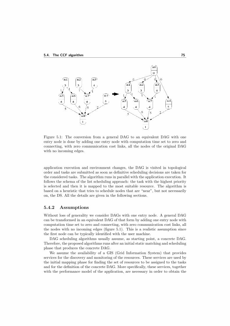
5.4. The CCF algorithm 75
Figure 5.1: The conversion from a general DAG to an equivalent DAG with oneentry node is done by adding one entry node with computation time set to zero andconnecting, with zero communication cost links, all the nodes of the original DAGwith no incoming edges.
application execution and environment changes, the DAG is visited in topologicalorder and tasks are submitted as soon as definitive scheduling decisions are taken forthe considered tasks. The algorithm runs in parallel with the application execution. Itfollows the schema of the list scheduling approach: the task with the highest priorityis selected and then it is mapped to the most suitable resource. The algorithm isbased on a heuristic that tries to schedule nodes that are “near”, but not necessarilyon, the DS. All the details are given in the following sections.
5.4.2 Assumptions
Without loss of generality we consider DAGs with one entry node. A general DAGcan be transformed in an equivalent DAG of that form by adding one entry node withcomputation time set to zero and connecting, with zero communication cost links, allthe nodes with no incoming edges (figure 5.1). This is a realistic assumption sincethe first node can be typically identified with the user machine.
DAG scheduling algorithms usually assume, as starting point, a concrete DAG.Therefore, the proposed algorithms runs after an initial static matching and schedulingphase that produces the concrete DAG.
We assume the availability of a GIS (Grid Information System) that providesservices for the discovery and monitoring of the resources. These services are used bythe initial mapping phase for finding the set of resources to be assigned to the tasksand for the definition of the concrete DAG. More specifically, these services, togetherwith the performance model of the application, are necessary in order to obtain the
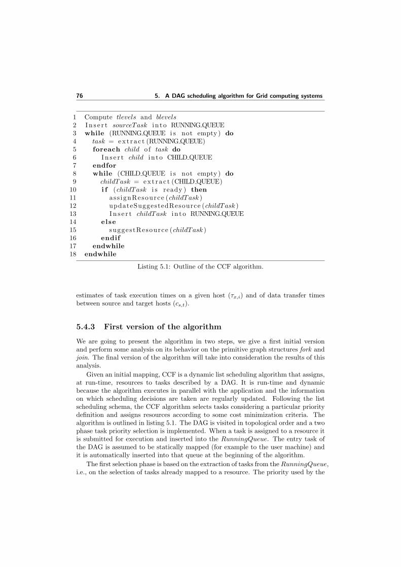
76 5. A DAG scheduling algorithm for Grid computing systems
1 Compute tlevels and blevels2 I n s e r t sourceTask i n t o RUNNING QUEUE3 while (RUNNING QUEUE i s not empty ) do4 task = ext ra c t (RUNNING QUEUE)5 foreach child o f task do6 I n s e r t child i n t o CHILD QUEUE7 endfor8 while (CHILD QUEUE i s not empty ) do9 childTask = ext ra c t (CHILD QUEUE)
10 i f (childTask i s ready ) then11 ass ignResource (childTask )12 updateSuggestedResource (childTask )13 I n s e r t childTask i n t o RUNNING QUEUE14 else15 suggestResource (childTask )16 endif17 endwhile18 endwhile
Listing 5.1: Outline of the CCF algorithm.
estimates of task execution times on a given host (τx,i) and of data transfer timesbetween source and target hosts (cs,t).
5.4.3 First version of the algorithm
We are going to present the algorithm in two steps, we give a first initial versionand perform some analysis on its behavior on the primitive graph structures fork andjoin. The final version of the algorithm will take into consideration the results of thisanalysis.
Given an initial mapping, CCF is a dynamic list scheduling algorithm that assigns,at run-time, resources to tasks described by a DAG. It is run-time and dynamicbecause the algorithm executes in parallel with the application and the informationon which scheduling decisions are taken are regularly updated. Following the listscheduling schema, the CCF algorithm selects tasks considering a particular prioritydefinition and assigns resources according to some cost minimization criteria. Thealgorithm is outlined in listing 5.1. The DAG is visited in topological order and a twophase task priority selection is implemented. When a task is assigned to a resource itis submitted for execution and inserted into the RunningQueue. The entry task ofthe DAG is assumed to be statically mapped (for example to the user machine) andit is automatically inserted into that queue at the beginning of the algorithm.
The first selection phase is based on the extraction of tasks from the RunningQueue,i.e., on the selection of tasks already mapped to a resource. The priority used by the
5.4. The CCF algorithm 77
RunningQueue is defined as:
Prio RQ(nx) = max{
tlevel(nx, hnx) + blevel(nx, hnx), DSdesc(nx)}
(5.1)
where hnx is the host assigned to the task nx and DSdesc(nx) is the value of thelongest path passing through a partially free descendant of nx. The value DSdesc
is set by the suggestResource() procedure and will be discussed later. The extractoperation returns (and removes from the queue) the task with the highest priorityvalue, which is the node belonging to the Dominant Sequence if the priority value isnot given by DSdesc(nx), otherwise it selects a node having a partially free DS nodeas descendant. Once a task is extracted from that queue all its children are insertedinto the ChildQueue.
The second selection phase empties this queue and assigns a resource for eachready child. The ChildQueue orders the tasks using the following priority:
Prio CQ(ny) = tlevel(ny, hny ) + blevel(ny, hny ) (5.2)
where hnyis the host assigned to ny by the initial mapping. The while loop in line 8
(listing 5.1) considers each child ny and checks if it is ready or not (i.e. all its parentsare mapped or not). In the first case (lines 11-13) a resource is assigned to the taskand it is inserted into the RunningQueue. The function updateSuggestedResouce()in line 12 will be explained later. If the task is not ready (line 15), this means thatsome of its parents are not mapped and the procedure suggestResource() suggests aresource (hnx
, the resource assigned to the father nx extracted in line 4) to all theunmapped parents.
Following this schema, children with one parent are immediately mapped to anappropriate resource, whereas children with more than one parent wait until all par-ents are scheduled. It should be noted that the first selection phase considers highpriority tasks in the RunningQueue, i.e. tasks with an already assigned resourcethat are, potentially, running. It is the second selection phase that looks for readytasks needing a resource. This approach is different from all the others used in listscheduling algorithms. In particular, the priority definition (5.1) needs some moreexplanation. The main objective is to select DS nodes. However, if the heaviestchild nh of a selected DS node is not ready, then it is not assigned to a resourceand waits until all its parents are mapped. Therefore, it is not guaranteed that thenext selected node from the RunningQueue will be a DS node, unless there is morethan one DS. The idea is to stay “near” the DS by making nh ready as soon aspossible. This happens when a task is selected from the RunningQueue because thevalue DSdesc is the maximum. DSdesc is initially set to zero for all the tasks and ispossibly updated by the suggestResource() procedure, which is discussed later. If nh
is not ready the second selection phase can choose non-DS tasks for mapping. Thismakes this heuristic a hybrid between CP-based and non-CP-based heuristic. Thenext paragraphs describe the mapping function assignResource() and the functionssuggestResource() and updateSuggestedResouce().
78 5. A DAG scheduling algorithm for Grid computing systems
The mapping function assignResource()
This function assigns a suitable resource to a task. There are two important aspects:the set of candidate resources and the cost function to minimize.
The set of the candidate resources C is composed by:
• the resource assigned by the initial static mapping to the task;
• the resources of the task parents;
• one suggested resource.
The suggested resource, if present, is defined by the functions suggestResource() andupdateSuggestedResource. The resource assigned by the initial static mapping is thereference resource, i.e. the one that gives the cost that have to be minimized. Thecost function of the task ny on a given host h, is defined as:
Cost(ny, h) = tlevel(ny, h) + blevel(ny, h).
The function assignResource() selects the resource that minimize this cost function,by testing ny on all the resources hi belonging to the set of candidate resources. Whenthe task ny is tested on the machine hi the cost function Cost(ny, hi) is computed asfollows:
1. the estimate of execution time of task ny on the host hi is computed (τy,i);
2. if a predecessor np is assigned to hi the edge (np, ny) is zeroed, otherwise theestimate of the data transfer time cp,y is recomputed.
3. if a successor ns is assigned (by the initial mapping) to hi the edge (ny, ns) iszeroed, otherwise the estimate of the data transfer time cy,s is recomputed.
For selected resource hny holds:
Cost(ny, hny) = min
hj∈C
{Cost(ny, hj)
}.
The suggestResource() and updateSuggestedResource() functions
The rationale behind the suggested resource is to increase the probability of zeroingmultiple incoming edges. Obviously, in order for a task to zero multiple incoming edgeswhen assigned to a machine, there must be more than one of its parents assigned tothe same machine. In figure 5.2 task n1 is selected from the RunningQueue and taskn6 is its heaviest child (the one laying on the CP, indicated by the thick arrow). n6
is not ready and it will be considered for scheduling only when all its parents aredefinitively assigned to a resource. At the moment of scheduling the task n6, therecould be an advantage if tasks n3, n4 and n5 are also assigned to hn1 . In some way,tasks n2, n3, n4 and n5 should be aware that they are converging towards one task(n6 in this case).
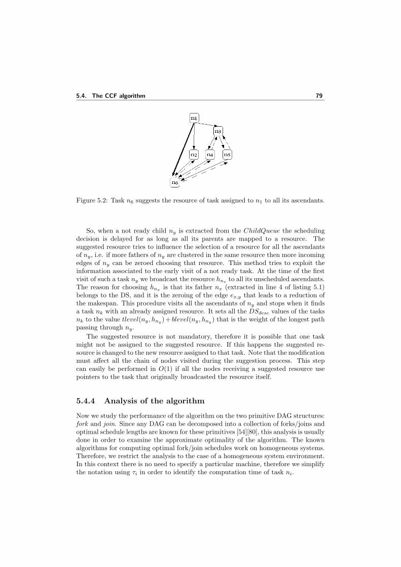
5.4. The CCF algorithm 79
Figure 5.2: Task n6 suggests the resource of task assigned to n1 to all its ascendants.
So, when a not ready child ny is extracted from the ChildQueue the schedulingdecision is delayed for as long as all its parents are mapped to a resource. Thesuggested resource tries to influence the selection of a resource for all the ascendantsof ny, i.e. if more fathers of ny are clustered in the same resource then more incomingedges of ny can be zeroed choosing that resource. This method tries to exploit theinformation associated to the early visit of a not ready task. At the time of the firstvisit of such a task ny we broadcast the resource hnx
to all its unscheduled ascendants.The reason for choosing hnx is that its father nx (extracted in line 4 of listing 5.1)belongs to the DS, and it is the zeroing of the edge ex,y that leads to a reduction ofthe makespan. This procedure visits all the ascendants of ny and stops when it findsa task nk with an already assigned resource. It sets all the DSdesc values of the tasksnk to the value tlevel(ny, hny )+ blevel(ny, hny ) that is the weight of the longest pathpassing through ny.
The suggested resource is not mandatory, therefore it is possible that one taskmight not be assigned to the suggested resource. If this happens the suggested re-source is changed to the new resource assigned to that task. Note that the modificationmust affect all the chain of nodes visited during the suggestion process. This stepcan easily be performed in O(1) if all the nodes receiving a suggested resource usepointers to the task that originally broadcasted the resource itself.
5.4.4 Analysis of the algorithm
Now we study the performance of the algorithm on the two primitive DAG structures:fork and join. Since any DAG can be decomposed into a collection of forks/joins andoptimal schedule lengths are known for these primitives [54][80], this analysis is usuallydone in order to examine the approximate optimality of the algorithm. The knownalgorithms for computing optimal fork/join schedules work on homogeneous systems.Therefore, we restrict the analysis to the case of a homogeneous system environment.In this context there is no need to specify a particular machine, therefore we simplifythe notation using τi in order to identify the computation time of task ni.
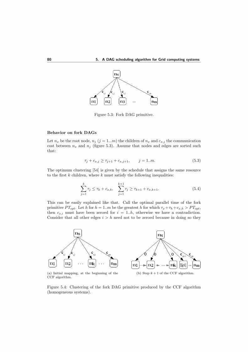
80 5. A DAG scheduling algorithm for Grid computing systems
Figure 5.3: Fork DAG primitive.
Behavior on fork DAGs
Let nx be the root node, nj (j = 1...m) the children of nx and cx,j the communicationcost between nx and nj (figure 5.3). Assume that nodes and edges are sorted suchthat:
τj + cx,j ≥ τj+1 + cx,j+1, j = 1..m. (5.3)
The optimum clustering [54] is given by the schedule that assigns the same resourceto the first k children, where k must satisfy the following inequalities:
k∑j=1
τj ≤ τk + cx,k,
k+1∑j=1
τj ≥ τk+1 + cx,k+1. (5.4)
This can be easily explained like that. Call the optimal parallel time of the forkprimitive PTopt. Let h for h = 1..m be the greatest h for which τx +τh +cx,h > PTopt,then cx,i must have been zeroed for i = 1..h, otherwise we have a contradiction.Consider that all other edges i > h need not to be zeroed because in doing so they
(a) Initial mapping, at the beginning of theCCF algorithm.
(b) Step k + 1 of the CCF algorithm.
Figure 5.4: Clustering of the fork DAG primitive produced by the CCF algorithm(homogeneous systems).
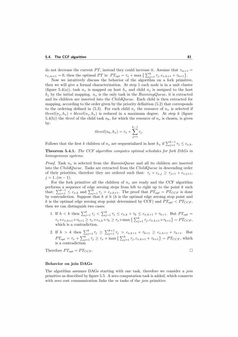
5.4. The CCF algorithm 81
do not decrease the current PT , instead they could increase it. Assume that τm+1 =cx,m+1 = 0, then the optimal PT is: PTopt = τx + max
{ ∑hj=1 τj , cx,h+1 + τh+1
}.
Now we intuitively discuss the behavior of the algorithm on a fork primitive,then we will give a formal characterization. At step 1 each node is in a unit cluster(figure 5.4(a)), task nx is mapped on host hx and child nj is assigned to the hosthj by the initial mapping. nx is the only task in the RunningQueue, it is extractedand its children are inserted into the ChildQueue. Each child is then extracted formapping, according to the order given by the priority definition (5.2) that correspondsto the ordering defined in (5.3). For each child nj the resource of nx is selected iftlevel(nj , hx) + blevel(nj , hx) is reduced in a maximum degree. At step k (figure5.4(b)) the tlevel of the child task nk, for which the resource of nx is chosen, is givenby:
tlevel(nk, hx) = τx +k−1∑j=1
τj .
Follows that the first k children of nx are sequentialized in host hx if∑k−1
j=1 τj ≤ cx,k.
Theorem 5.4.1. The CCF algorithm computes optimal schedules for fork DAGs inhomogeneous systems.
Proof. Task nx is selected from the RunninQueue and all its children are insertedinto the ChildQueue. Tasks are extracted from the ChildQueue in descending orderof their priorities, therefore they are ordered such that: τj + cx,j ≥ τj+1 + cx,j+1,j = 1..(m− 1).
For the fork primitive all the children of nx are ready and the CCF algorithmperforms a sequence of edge zeroing steps from left to right up to the point k suchthat:
∑k−1j=1 ≤ cx,k and
∑kj=1 τj > cx,k+1. The proof that PTopt = PTCCF is done
by contradiction. Suppose that k 6= h (h is the optimal edge zeroing stop point andk is the optimal edge zeroing stop point determined by CCF) and PTopt < PTCCF ,then we can distinguish two cases:
1. If h < k then∑h
j=1 τj <∑k
j=1 τj ≤ cx,k + τk ≤ cx,h+1 + τh+1. But PTopt =
τx+cx,h+1+τh+1 ≥ τx+cx,k+τk ≥ τx+max{ ∑k
j=1 τj , cx,k+1+τk+1
}= PTCCF ,
which is a contradiction.
2. If h > k then∑h
j=1 τj ≥∑k+1
j=1 τj > cx,k+1 + τk+1 ≥ cx,h+1 + τh+1. But
PTopt = τx +∑h
j=1 τj ≥ τx + max{ ∑k
j=1 τj , cx,k+1 + τk+1
}= PTCCF , which
is a contradiction.
Therefore PTopt = PTCCF .
Behavior on join DAGs
The algorithm assumes DAGs starting with one task, therefore we consider a joinprimitive as described by figure 5.5. A zero computation task is added, which connectswith zero cost communication links the m tasks of the join primitive.
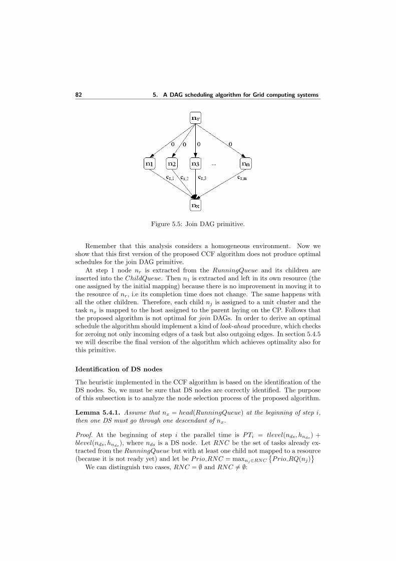
82 5. A DAG scheduling algorithm for Grid computing systems
Figure 5.5: Join DAG primitive.
Remember that this analysis considers a homogeneous environment. Now weshow that this first version of the proposed CCF algorithm does not produce optimalschedules for the join DAG primitive.
At step 1 node nr is extracted from the RunningQueue and its children areinserted into the ChildQueue. Then n1 is extracted and left in its own resource (theone assigned by the initial mapping) because there is no improvement in moving it tothe resource of nr, i.e its completion time does not change. The same happens withall the other children. Therefore, each child nj is assigned to a unit cluster and thetask nx is mapped to the host assigned to the parent laying on the CP. Follows thatthe proposed algorithm is not optimal for join DAGs. In order to derive an optimalschedule the algorithm should implement a kind of look-ahead procedure, which checksfor zeroing not only incoming edges of a task but also outgoing edges. In section 5.4.5we will describe the final version of the algorithm which achieves optimality also forthis primitive.
Identification of DS nodes
The heuristic implemented in the CCF algorithm is based on the identification of theDS nodes. So, we must be sure that DS nodes are correctly identified. The purposeof this subsection is to analyze the node selection process of the proposed algorithm.
Lemma 5.4.1. Assume that nx = head(RunningQueue) at the beginning of step i,then one DS must go through one descendant of nx.
Proof. At the beginning of step i the parallel time is PTi = tlevel(nds, hnds) +
blevel(nds, hnds), where nds is a DS node. Let RNC be the set of tasks already ex-
tracted from the RunningQueue but with at least one child not mapped to a resource(because it is not ready yet) and let be Prio RNC = maxnj∈RNC
{Prio RQ(nj)
}We can distinguish two cases, RNC = ∅ and RNC 6= ∅:
5.4. The CCF algorithm 83
1. If RNC = ∅ then Prio RQ(nx) = tlevel(nx, hnx) + blevel(nx, hnx) is the maxi-mum on all the nodes in the RunningQueue and nx is a DS node itself. Followsthat at least one child of nx must lay in one DS.
2. If RNC 6= ∅ then Prio RQ(nx) ≤ Prio RNC. Now we have two cases:
(a) If Prio RQ(nx) = Prio RNC then either nx is a DS node itself (and thereis more than one DS) or Prio RQ(nx) is given by the value DSdesc, setby the heaviest child nh (which is not ready) of a task in the set RNC,through the suggestResource() procedure. nh is also a descendant of nx.
(b) If Prio RQ(nx) < Prio RNC then if Prio RQ(nx) = tlevel(nx, hnx) +blevel(nx, hnx) nx is a DS node itself. Otherwise, if Prio RQ(nx) =DSdesc(nx) then the DS passes through a not ready child nk of a taskin the set RNC, but, since DSdesc(nx) was set by the suggestResource()procedure starting from nk, nk is a descendant of nx.
Lemma 5.4.1 states that the first selection phase considers nodes belonging to theDS or nodes having, as descendant, a partially free DS node. In the latter case, thepurpose is to make a partially free DS node ready as soon as possible.
Monotone reduction of the schedule length
The node ni extracted from the RunningQueue has the maximum value of tlevel +blevel. The mapping phase assigns resources to all the ready children of ni, eachtime zeroing one or more incoming edges, provided that the schedule length does notincrease. If one step of the algorithm is identified with both the extraction of a DSnode from the RunningQueue and the mapping of all the ready children, then theproperty of monotone reduction of the schedule length holds, i.e. for each step i ofthe algorithm PTi−1 ≥ PTi, where PTi is the parallel time at step i (weight of theDS at a given step i).
Theorem 5.4.2. For each step i of the CCF algorithm PTi ≥ PTi+1
Proof. The parallel time at step i can be computed as: PTi = maxnj∈V
{tlevel(nj , hnj )+
blevel(nj , hnj)}. At step i a node nx is extracted from the RunningQueue. All chil-
dren of nx are assigned to a temporary resource and now the algorithm tries to assigna definitive resource to all the ready children nr. The temporary resource ht of a childis going to change to a new resource hn if:
tlevel(nr, hn) + blevel(nr, hn) < tlevel(nr, ht) + blevel(nr, ht).
Given this, since PT = maxnj∈V
{tlevel(nj , hnj
) + blevel(nj , hnj)}
and PTi andPTi+1 are computed, respectively, before and after the definitive mapping of theready children, follows that: PTi ≥ PTi+1.

84 5. A DAG scheduling algorithm for Grid computing systems
5.4.5 Final version of the algorithm
The final version of the algorithm aims at reaching the optimality also for the joinDAG structure. As we will see in the experimental results section this modification,combined with the suggestResource() process (section 5.4.3), leads to an improve-ment of the quality of the scheduling produced, i.e., to a reduction of the makespan. Toachieve this goal the final version of the algorithm implements, in the assignResource()function, a look-ahead strategy, similar to the one used in the DCP algorithm [78]. Inparticular, we first try to select a resource basing the decision on the minimization ofthe cost function tlevel + blevel of the task nj (described in section 5.4.3) then, if theschedule length is not reduced, the assignResource() procedure is repeated, but thistime trying to virtually schedule the heaviest child nhc of nj (the one that determinesthe blevel of nj) in the same resource. Finally, a suggestResource() is called fromnhc suggesting the resource selected for nj to all the unmapped ascendants. Thelook-ahead strategy defines the cost function as follows:
Cost(nj , h) = tlevel(nj , h) + blevel(nj , h)+ tlevel(nhc, h) + blevel(nhc, h)
where nhc is the heaviest child of nj and h the resource that is under examination.In this way, the selected resource for nj tries to maximize the probability of zeroingmultiple edges for its heaviest child. With this look-ahead strategy, combined with theresource suggestion process, the algorithm achieves the optimality for the DAG joinprimitive and experimental tests show improvements on the length of the scheduleproduced. On the other side, the monotone reduction property does not hold anymore.This happens because the resource is selected considering the estimate reduction of theschedule length, given by virtually mapping the heaviest child on the same resource.The mapped task is nj (not nhc) and the variation in tlevel(nj , h) + blevel(nj , h) isthe one that concretely affects the schedule length. Therefore, when mapping nj itcan happen that the total schedule length increases. Since the future mapping ofthe heaviest child does not guarantee a reduction greater than the increment possiblyobtained before, the monotone reduction property does not hold anymore. We haveexperimentally found that if the look-ahead strategy is applied systematically eachtime a resource is selected (like in the DCP algorithm) then there is no improvementby using this technique. Otherwise, if it is used only on a restricted class of events thengood results can be obtained. The proposed algorithm uses the look-ahead strategyonly in the case in which the schedule length is not reduced by the mapping function,and experimental results show a good improvement in the quality of the scheduleproduced.
The optimality for the fork DAG primitive still holds for this final version and thenext paragraph shows how the optimality for the join primitive is obtained.
The suggestResource() function
In the final version of the algorithm, with the introduction of the look-ahead process,the suggested resource plays a central role. Now we can see why its effect is to
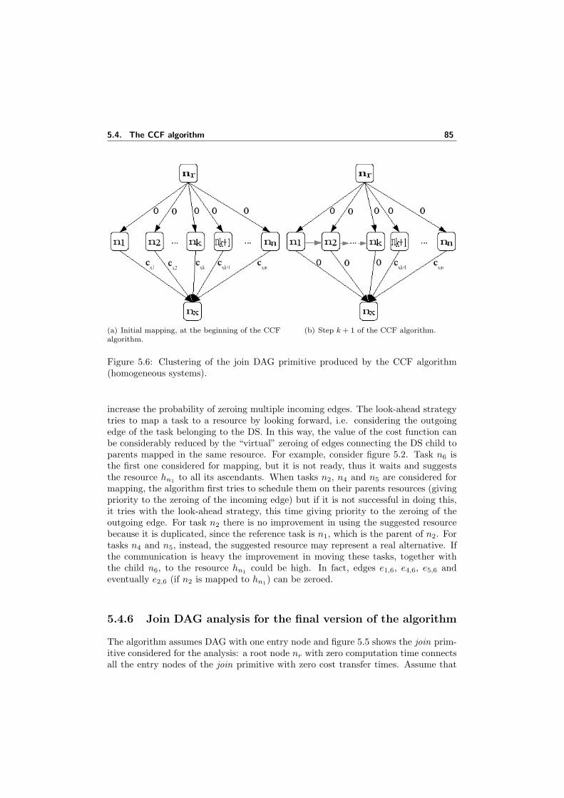
5.4. The CCF algorithm 85
(a) Initial mapping, at the beginning of the CCFalgorithm.
(b) Step k + 1 of the CCF algorithm.
Figure 5.6: Clustering of the join DAG primitive produced by the CCF algorithm(homogeneous systems).
increase the probability of zeroing multiple incoming edges. The look-ahead strategytries to map a task to a resource by looking forward, i.e. considering the outgoingedge of the task belonging to the DS. In this way, the value of the cost function canbe considerably reduced by the “virtual” zeroing of edges connecting the DS child toparents mapped in the same resource. For example, consider figure 5.2. Task n6 isthe first one considered for mapping, but it is not ready, thus it waits and suggeststhe resource hn1 to all its ascendants. When tasks n2, n4 and n5 are considered formapping, the algorithm first tries to schedule them on their parents resources (givingpriority to the zeroing of the incoming edge) but if it is not successful in doing this,it tries with the look-ahead strategy, this time giving priority to the zeroing of theoutgoing edge. For task n2 there is no improvement in using the suggested resourcebecause it is duplicated, since the reference task is n1, which is the parent of n2. Fortasks n4 and n5, instead, the suggested resource may represent a real alternative. Ifthe communication is heavy the improvement in moving these tasks, together withthe child n6, to the resource hn1 could be high. In fact, edges e1,6, e4,6, e5,6 andeventually e2,6 (if n2 is mapped to hn1) can be zeroed.
5.4.6 Join DAG analysis for the final version of the algorithm
The algorithm assumes DAG with one entry node and figure 5.5 shows the join prim-itive considered for the analysis: a root node nr with zero computation time connectsall the entry nodes of the join primitive with zero cost transfer times. Assume that
86 5. A DAG scheduling algorithm for Grid computing systems
nodes and edges are sorted such that:
τj + cj,x ≥ τj+1 + cj+1,x j = 1..m− 1. (5.5)
As for the fork primitive, the optimum clustering [80] is a tradeoff between paral-lelization and sequentialization; it is given by the schedule that clusters together thefirst k nodes nj , where k must satisfy the following inequalities:
k∑j=1
τj ≤ τk + ck,x,
k+1∑j=1
τj ≥ τk+1 + ck+1,x.
The first node in the RunningQueue, nr, is extracted and all its children nj (j = 1..m)are inserted into the ChildQueue. Since all the communication costs cr,j are zero,tasks nj are extracted from the ChildQueue following the order given by their blevelthat corresponds to the order defined in (5.5). Task n1 is extracted and, since there isno improvement in assigning it to hr, the look-ahead strategy is called. The resourceassigned to n1 is still hn1 but this time the suggestResource() suggests resource hn1
to all the nj . The look-ahead strategy is called for all the remaining tasks and cj,x
is checked for zeroing by virtually mapping nx to the suggested resource. The firstk nodes are sequentialized on the suggested resource if
∑k−1j=1 τj,hn1
≤ ck,x. Finally,task nx is assigned to hn1 since its first k incoming edges can be zeroed.
Theorem 5.4.3. The final version of the CCF algorithm computes optimal schedulesfor join DAGs in homogeneous systems.
Proof. Task nr is selected from the RunninQueue and all its children are insertedinto the ChildQueue. Tasks are extracted from the ChildQueue in descending orderof their priorities, therefore they are ordered such that: τj + cj,x ≥ τj+1 + cj+1,x,j = 1..(m − 1). The ChildQueue orders the tasks on the sum tlevel + blevel. Sincethe incoming edges of the tasks nj have a label value of zero, the blevel, and hencethe outgoing edge weight, is the one that affects the ordering.
The first task n1 is extracted from the ChildQueue and the assignResource()function tries to schedule it on the resource of its father. There is no improvement inmoving n1, therefore the look-ahead procedure is called. Also this time the resourceof the father nr and the resource hn1 , assigned to n1 by the initial mapping, givethe same value for the cost function and task n1 is definitively mapped to hn1 . ThesuggestResource() function is called and the resource hn1 is suggested to all theother tasks nj , j = 1...n. Now task n2 is extracted from the ChildQueue and, likewas happened for n1, it tested of its father resource with no improvements and thelook-ahead strategy is called. The algorithm finds that the cost function is minimizedon the suggested resource hn1 , because nx is virtually mapped to hn1 and two edgescan be zeroed. This process goes on by mapping tasks nj to the resource hn1 whileperforming a sequence of (virtual) edge zeroing steps from left to right up to the pointk such that:
∑k−1j=1 ≤ ck,x and
∑kj=1 τj > ck+1,x.
The proof that PTopt = PTCCF is done by contradiction. Suppose that k 6= h (his the optimal edge zeroing stop point and k is the optimal edge zeroing stop pointdetermined by CCF) and PTopt < PTCCF , then we can distinguish two cases:
5.5. A variant of the DSC algorithm 87
1. If h < k then∑h
j=1 τj <∑k
j=1 τj ≤ ck,x + τk ≤ ch+1,x + τh+1. But PTopt =
τx+ch+1,x+τh+1 ≥ τx+ck,x+τk ≥ τx+max{ ∑k
j=1 τj , ck+1,x+τk+1
}= PTCCF ,
which is a contradiction.
2. If h > k then∑h
j=1 τj ≥∑k+1
j=1 τj > ck+1,x + τk+1 ≥ ch+1,x + τh+1. But
PTopt = τx +∑h
j=1 τj ≥ τx + max{ ∑k
j=1 τj , ck+1,x + τk+1
}= PTCCF , which
is a contradiction.
Therefore PTopt = PTCCF .
5.5 A variant of the DSC algorithm
In this section we propose a variant of the DSC (Dominant Sequence Clustering)algorithm. First of all we briefly recall how the original algorithm works. The DSC[135] selects at each step a node belonging to the DS, the critical path of the scheduledDAG computed as the maximum value of tlevel + blevel, and assigns it to the resourcethat allows the minimum start time. In this first version the algorithm is simple andit achieves good results but it is not optimal for join DAGs. The authors formulate afinal version adding two features: the possibility to cluster together already scheduledparents of a node and the possibility to book a resource for a partially free node(a node for which only some of its parents are visited) belonging to the DS. Thefinal version of the algorithm achieves optimality also for join DAGs (in homogeneoussystems). We have adapted the DSC algorithms in order to work in a heterogeneousenvironment and we have tested the two versions of the algorithm with random DAGsand different network topologies. The results showed no real improvements from thefirst and the final version of the algorithm, on average the first version performs betterthan the final one.
Here we propose a variant of the DSC algorithm that leverages from some con-cepts used in the final version of the CCF algorithm. In particular, we take the firstversion of the DSC algorithm and we add the look-ahead strategy together with thesuggestResource() function. These two features are integrated as follows:
1. Like for the CCF algorithm the look-ahead process is called only when thealgorithm does not find a better resource than the one assigned by the initialmapping.
2. The suggestResource() function is used only when a resource is selected withthe look-ahead process. In particular, the child task that is virtually mapped tothe resource just assigned to the father task, is the one that calls this function.
The result is a variant of the DSC algorithm for which some of the properties ofthe original DSC algorithm still holds, like optimal behavior on fork and join DAGsin homogeneous systems and the correctness in locating DS nodes. Due to the look-ahead strategy, like for the CCF algorithm, the monotone reduction property of theschedule length does not hold anymore and the time complexity of this new variantof the DSC algorithm is no longer O((v + e) log v).
88 5. A DAG scheduling algorithm for Grid computing systems
As can be seen in the next chapter experimental results show significant improve-ments on the length of the schedules produced, i.e. reduction of the makespan.
5.6 Summary
In this chapter we have presented two new DAG scheduling algorithms designed towork in a Grid computing system, which is a heterogeneous computing system witha heterogeneous interconnection network.
The first proposed algorithm is called CCF (Cluster ready Children First)and itis a list scheduling algorithm. It visits the DAG in topological order and uses a twostep node selection phase based on a priority that identifies tasks belonging to theDominant Sequence, if it is possible, otherwise means that the next DS task is blockedbecause it is not ready and in this case it is selected the task (or a sequence of tasks)allowing the DS node to become ready as soon as possible. More specifically, the firststep selects a running task (i.e., already mapped) and then all the ready children ofthat task are selected for mapping. This selection of tasks is different from all the otherlist scheduling approaches. The first selection step considers already mapped tasksand in the second step can happen that only non-DS tasks are mapped. This makesthis heuristic a hybrid between CP-based and non CP-based. Then, the final versionof the algorithm, introduces a process for adding a particular resource to the set ofcandidate resources (the set from which the best resource for a task is drawn) anda look-ahead strategy is invoked when the algorithm does not find a better resourceother than the initial mapping.
Some properties of the proposed CCF algorithm are identified and analyzed, suchas the optimal behavior on fork and join DAGs in homogeneous systems, monotonereduction of the schedule length (first version of the algorithm) and the correct iden-tification of DS nodes.
The second proposed algorithm, the DSC VAR, is a variant of the famous DSC.DSC VAR adds to the first version of the original algorithm the resource suggestionprocess and the look-ahead strategy used in the CCF algorithm. Some of the proper-ties of the original version still hold for this variant, like the optimal behavior on forkand join DAGs in homogeneous systems.
The next chapter describes experimental results conducted with these two algo-rithms. Random DAGs and different network topologies are used in order to comparethe results of the proposed algorithms with other two algorithms: the original DSCand the Hybrid Remapper. The platforms describing the heterogeneous computingenvironment used in the simulations are created using the GridG toolkit. As we willsee, the performance comparison shows improvements on the length of the schedulesproduced by the two proposed algorithms, both for poor and good initial mappings.

6Experimental Results
Scheduling the tasks of a distributed application has been an active field of research forseveral decades. The classic scheduling problem is to find an assignment of applicationtasks onto a set of distributed resources with the aim of minimizing the makespan, i.e.the overall completion time of the parallel application. As we have seen in previouschapters, it has been shown that non-trivial instances of the DAG scheduling problemare NP-complete. As a result, the researchers have proposed different approaches tosolve the problem. However it is difficult to determine which solutions are practicalfor real scenarios. Given the NP-completeness nature of the problem, it is really hardto make a theoretical evaluation of the different proposed heuristics. On the otherhand, studying the behavior of scheduling algorithms on real platforms, althoughproviding accurate and undoubtedly realistic results, is not practical due the dynamicavailability of the resources. The main problem is that experiments on real platformsare often non-reproducible, this means that results of different scheduling algorithmsare not comparable. Therefore, simulation is the best choice in order to test andcompare scheduling algorithms.
This chapter presents experimental results obtained with the simulation of theproposed algorithms CCF and DSC VAR, which are compared to the original DSC[135] and the Hybrid Remapper [90] algorithms.
6.1 Simulation framework
We have conducted extensive simulations to evaluate the performance of the twoproposed scheduling algorithms. In particular, we present a comparison of the per-formance results of the CCF and DSC VAR algorithms with other two schedulingalgorithms, the original DSC [135] described in section 4.6.9 and the Hybrid Remap-per [90] described in section 4.6.14. The Hybrid Remapper is presented by its authorsin three versions called PS, CS and CD. Here we use the third version (CD), whichis the one that considers dynamic values in the computation of priorities.
The input to the simulator consists of a set of DAGs and an environment descrip-tion of the network and the resources (the platform). Each scheduling algorithm canretrieve informations like: machine characteristics, latency and bandwidth. In thefollowing the experimental session will be described considering three main areas: the
90 6. Experimental Results
simulator, DAG generation and platform generation. Finally results and commentsof the performance comparison are presented.
6.1.1 The simulator
We evaluated three simulators: GridSim [15], Simgrid [17, 81, 65] and MetaSimgrid[82]. With Simgrid it is possible to model a platform and defining arbitrary topologyfor the interconnection network, whereas with GridSim this cannot be done. Onthe other hand with Simgrid the platform model must be constructed by hand; itcan be done for few hosts, but for more realistic cases it is practically impossible.Furthermore, Simgrid lacks a number of convenient features to craft simulations of adistributed application where scheduling decisions are not taken by a single process.MetaSimgrid is a Grid simulation tool build on top of Simgrid that overcomes to somelimitations of Simgrid. For example, it is possible to import an existing platform. Inthis way, it is possible to use existing tools for building platforms with approximatelyrealistic topology, including switches and routers, and to gather data on its availableresources. Examples of such a tools are:
• ENV with NWS: ENV (Effective Network View) [113] allows to discover theeffective topology of a network from a given host, whereas NWS (NetworkWeather System) [130] can be used to gather all the traces (link latency, band-width, cPU load, etc.) needed to simulate external load.
• GridG with Tier: GridG [88] is a toolkit based on Tier [16, 33]. With this toolkitit is possible to easily generate approximately realistic plaforms with arbitrarynetwork topology and resources characteristics.
Our final choice was to use MetaSimgrid for the simulation of the algorithms and theGridG toolkit for the generation of the test platforms.
6.1.2 DAG generation
Due to the NP-completeness of this scheduling problem, heuristic ideas used in CCFand DSC VAR cannot always lead to an optimal solution. Thus it is necessary tocompare the average performance of different algorithms using randomly generatedgraphs.
We have generated each DAG at random, starting from he following input pa-rameters: number of nodes, number of edges, range (minimum and maximum) ofcomputation values and range of data transfer values. These values are abstract la-bels (number of operations and size of data). We are dealing with DAGs, thereforethe number of edges |E| is limited by:
|E| ≤ |V |(|V | − 1)/2
where |V | is the number of nodes. Random edges (i, j) are generated with i < j.Nodes and edges labels are generated at random and their values are drawn from thecorresponding ranges given as input. Abstract labels are transformed in time values
6.1. Simulation framework 91
by the scheduling algorithm once the characteristics of the resources are known. Inparticular, in order to obtain the estimate of the execution time of a task, we haveto retrieve the CPU speed (given in mips) and to divide the abstract label associatedto that task by the CPU speed. Analogously, in order to obtain the estimate of thetransfer time we have to retrieve the link characteristics (latency and bandwidth) andto perform this simple operation:
Transfer time estimate = latency + (data size/bandwidth).
The Communication Computation Ratio (CCR) is defined as the average edgeweight divided by the average node weight. DAGs with a CCR smaller than 1 arecalled coarse grain DAGs and DAGs with a CCR grater than 1 are called fine grainDAGs. All the DAGs used for the tests are divided into two groups: the first groupcontains coarse grain DAGs with a CCR ranging from 0.05 up to 1 and the secondgroup contains fine grain DAGs with a CCR ranging from 1 up to 20. Each groupis divided into 30 subgroups, each containing 20 DAGs with (approximately) thesame CCR. The CCR of the 30 subgroups progressively increases from subgroup 1 tosubgroup 30, i.e. from 0.05 to 1 for the coarse grain DAGs and from 1 to 20 for thefine grain DAGs.
6.1.3 Platform generation
A realistic platform is essential in evaluating middleware for computational grids.The platform is the raw Grid, an annotated graph representing the network topologyand the hardware and software available on each node and link within it. For thegeneration of the network topology and the definition of the characteristics of theresources we have used the GridG toolkit [88]. It leverages from Tier [16, 33], atool for network topology generation, extending it in order to produce graphs thatconform to recently discovered power laws of Internet topology [37]. In general, aGrid generator has to produce a grid of a given number of hosts and must meet thefollowing requirements:
• Realistic network topology : real network topologies are connected and have hi-erarchical structures. Furthermore recent studies found that wide area networktopologies follow certain topological power laws.
• Realistic annotations for hosts and network components: that means providingfundamental characteristics for hosts, links, routers and switches. For hostssuch characteristics are: architecture type, processor type and speed, numberof processors, memory size, disk size, hardware vendor, operating system, andavailable software. For a link, it should provide the hardware bandwidth andlatency. For routers and switches, it should specify the aggregate backplane orswitching fabric throughput and latency. Furthermore, characteristics of differ-ent components are often correlated, e.g. memory size increases with processorspeed, a high speed router is unlikely to be connected only to a few slow links,and so on.
92 6. Experimental Results
Rank exponent dv ∝ rRv
Power Laws Outdegree exponent fd ∝ dO
Eigen exponent λi ∝ iε
Approximation Hop-plot exponent P (h) ∝ hH
Table 6.1: Power laws of Internet topology [88, 37].
GridG starts with the output of a structure-oriented topology generator (they cur-rently use Tiers [16, 33]) and adds redundancy to it in such a way as to make itconform to the power laws. Table 6.1 summarizes the three power laws identified byFaloutsos et al. in [37]. Faloutsos defines the rank of a node in the following way.First the nodes are sorted in decreasing order of out-degree, then ranks are assignedaccording to this ordering and the number of nodes in each equivalence class (classesgroup nodes with the same out-degree). Nodes belonging to the highest out-degreeclass have rank rv = 1, nodes belonging to the second highest out-degree class haverank rv = 1 + (number of nodes in the previous class).
The rank exponential law says that the out-degree dv of a node v, is proportionalto the rank of the node (rv) raised to the power of a constant R.
The out-degree exponent law says that the frequency fd of an out-degree d isproportional to the out-degree raised to the power of a constant O.
The Eigen exponent power law says that the eigenvalues λi of a graph are propor-tional to the order i raised to the power of a constant ε.
The hop-plot exponent power law is considered as an approximation and says thatthe total number of pairs of nodes P (h), within h hops, is proportional to the numberof hops raised to the power of a constant H.
With the GridG toolkit we have created different platforms with the numberof resources ranging from 90 to 614. In order to consider different conditions ofenvironment load, for each platform we have generated 10 variants with weights (cpuand bandwidth) reduced at random by a percentage that ranges from 10% (for thefirst variant) to 95% (for the last variant). Final execution times for a platform arean average of the execution times on the variants.
6.2 Performance comparisons
As mentioned above the performance comparison of the proposed algorithms is madeusing two input sets: the first containing coarse grain DAGs (CCR smaller than 1) andthe second containing fine grain DAGs (CCR greater than 1). Tests were performedover different network topologies; here we present results for a platform formed by160 resources. For each single simulation the execution times are computed as anaverage of the execution of the 20 DAGs of each subgroup, having different numberof nodes and edges but with, approximately, the same CCR. In order to considerdifferent loads of the environment, each simulation is repeated 10 times with different
6.2. Performance comparisons 93
(a) Results for InitMap, DSC, CD, DSC VARand CCF.
(b) Results for DSC, CD, DSC VAR and CCF.
Figure 6.1: Results for CCR ranging from 0.05 to 1.
values of loads for the machines and the network, and the final execution time, for agiven CCR, is the average of the 10 simulations.
All the algorithms considered run over an initial mapping, which assigns a resourceto each task. We call the algorithm that implements this initial step the InitMap. Allthe considered scheduling algorithms try to improve this initial schedule. We use animplementation of the InitMap that visits the DAG in topological order and assignsto each task the resource that allows the earliest start time for that task. In order tostudy how the proposed heuristics can improve an initial bad mapping we have addedthe constraint of using a resource only once. At the end of this section we will considerhow the scheduling algorithms behave on an improved version of the InitMap.
Figure 6.1 shows the results for an increasing CCR ranging from 0.05 to 1. Inparticular, figure 6.1a considers all the tested algorithms, whereas figure 6.1b excludes
(a) Results for Initial mapping, ETF, DSC,CD, DSC VAR and CCF.
(b) Results for DSC, CD, DSC VAR andCCF.
Figure 6.2: Results for CCR ranging from 1 to 20.

94 6. Experimental Results
(a) Coarse grain DAGs (CCR smaller than 1). (b) Fine grain DAGs, (CCR greater than 1).
Figure 6.3: Comparison between the first version and the final version of the CCFalgorithm.
the InitMap algorithm in order to focus on the results of the other algorithms. Theresults for DSC, CD, DSC VAR and CCF are close to each other, but the proposedCCF and DSC VAR outperform, on average, all the other algorithms, as can beseen from figure 6.1b. For coarse grain DAGs the difference is small, in particularthe DSC VAR is very close to the CD algorithm. The original version of the DSCalgorithm perform worse than proposed variant DSC VAR.
Figure 6.2 considers simulation results for fine grain DAGs, where the averagecommunication time is greater than the average computation time. Figure 6.2a showsthe results of all the tested algorithms and figure 6.2b focuses on the DSC, CD,DSC VAR and CCF algorithms. Also for this class of DAGs the DSC VAR andCCF algorithms outperform, on average, all the other algorithms. In particular theimprovement gained by these two algorithms is higher than in the case of coarse grainDAGs. This result is mainly due to the application of the looking-ahead strategy,which optimizes the selection of a resource considering the amount of communicationbetween a task and its heaviest child, together with the suggestion resource process,which tracks the resource that allows to increase the probability of zeroing multipleincoming edges of the heaviest child. As can be seen, the improvement gained increaseswith the CCR. The DSC VAR still performs better of the original version of DSC.
Figure 6.3 shows the performance results of the first and final version of the CCFalgorithm. Remember that the final version differs from the first version becauseit implements the looking-ahead strategy, with the aim to reduce the makespan byreducing communication times. For coarse grain DAGs (figure 6.3(a)), where theaverage computation is higher than the average communication, the two versionsperform almost the same but, as the CCR increases, and hence the communicationgets higher, the final version of the algorithm outperforms the first version (figure6.3(b)). The looking-ahead strategy is applied only when the normal selection phasedo not find a better resource than the one chosen by the initial mapping. This pointis crucial. As we noted in section 5.4.5, the DCP algorithm [78] implements a similar
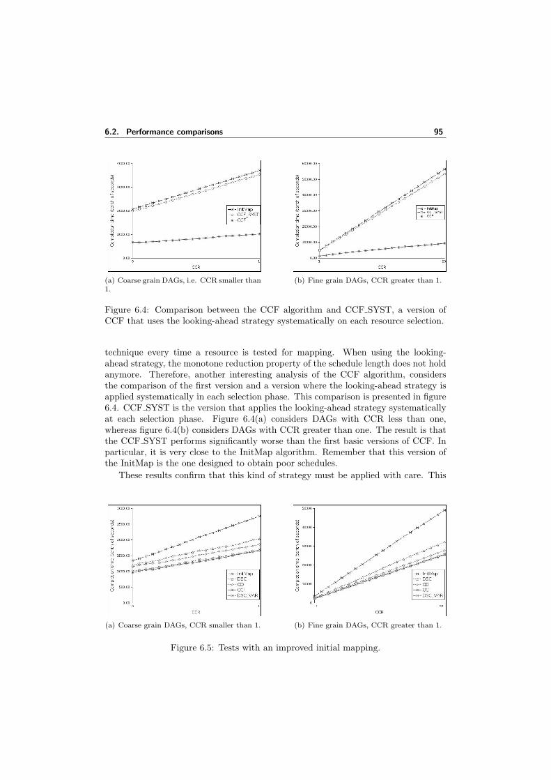
6.2. Performance comparisons 95
(a) Coarse grain DAGs, i.e. CCR smaller than1.
(b) Fine grain DAGs, CCR greater than 1.
Figure 6.4: Comparison between the CCF algorithm and CCF SYST, a version ofCCF that uses the looking-ahead strategy systematically on each resource selection.
technique every time a resource is tested for mapping. When using the looking-ahead strategy, the monotone reduction property of the schedule length does not holdanymore. Therefore, another interesting analysis of the CCF algorithm, considersthe comparison of the first version and a version where the looking-ahead strategy isapplied systematically in each selection phase. This comparison is presented in figure6.4. CCF SYST is the version that applies the looking-ahead strategy systematicallyat each selection phase. Figure 6.4(a) considers DAGs with CCR less than one,whereas figure 6.4(b) considers DAGs with CCR greater than one. The result is thatthe CCF SYST performs significantly worse than the first basic versions of CCF. Inparticular, it is very close to the InitMap algorithm. Remember that this version ofthe InitMap is the one designed to obtain poor schedules.
These results confirm that this kind of strategy must be applied with care. This
(a) Coarse grain DAGs, CCR smaller than 1. (b) Fine grain DAGs, CCR greater than 1.
Figure 6.5: Tests with an improved initial mapping.
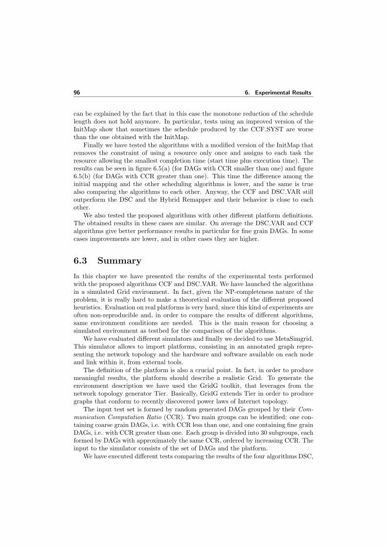
96 6. Experimental Results
can be explained by the fact that in this case the monotone reduction of the schedulelength does not hold anymore. In particular, tests using an improved version of theInitMap show that sometimes the schedule produced by the CCF SYST are worsethan the one obtained with the InitMap.
Finally we have tested the algorithms with a modified version of the InitMap thatremoves the constraint of using a resource only once and assigns to each task theresource allowing the smallest completion time (start time plus execution time). Theresults can be seen in figure 6.5(a) (for DAGs with CCR smaller than one) and figure6.5(b) (for DAGs with CCR greater than one). This time the difference among theinitial mapping and the other scheduling algorithms is lower, and the same is truealso comparing the algorithms to each other. Anyway, the CCF and DSC VAR stilloutperform the DSC and the Hybrid Remapper and their behavior is close to eachother.
We also tested the proposed algorithms with other different platform definitions.The obtained results in these cases are similar. On average the DSC VAR and CCFalgorithms give better performance results in particular for fine grain DAGs. In somecases improvements are lower, and in other cases they are higher.
6.3 Summary
In this chapter we have presented the results of the experimental tests performedwith the proposed algorithms CCF and DSC VAR. We have launched the algorithmsin a simulated Grid environment. In fact, given the NP-completeness nature of theproblem, it is really hard to make a theoretical evaluation of the different proposedheuristics. Evaluation on real platforms is very hard, since this kind of experiments areoften non-reproducible and, in order to compare the results of different algorithms,same environment conditions are needed. This is the main reason for choosing asimulated environment as testbed for the comparison of the algorithms.
We have evaluated different simulators and finally we decided to use MetaSimgrid.This simulator allows to import platforms, consisting in an annotated graph repre-senting the network topology and the hardware and software available on each nodeand link within it, from external tools.
The definition of the platform is also a crucial point. In fact, in order to producemeaningful results, the platform should describe a realistic Grid. To generate theenvironment description we have used the GridG toolkit, that leverages from thenetwork topology generator Tier. Basically, GridG extends Tier in order to producegraphs that conform to recently discovered power laws of Internet topology.
The input test set is formed by random generated DAGs grouped by their Com-munication Computation Ratio (CCR). Two main groups can be identified: one con-taining coarse grain DAGs, i.e. with CCR less than one, and one containing fine grainDAGs, i.e. with CCR greater than one. Each group is divided into 30 subgroups, eachformed by DAGs with approximately the same CCR, ordered by increasing CCR. Theinput to the simulator consists of the set of DAGs and the platform.
We have executed different tests comparing the results of the four algorithms DSC,

6.3. Summary 97
Hybrid Remapper, CCF and DSC VAR considering different platforms and differentinitial mappings. On average, the two proposed algorithms CCF and DSC VAR haveoutperformed the other two reference algorithms Hybrid Remapper and DSC. Wehave also proposed some tests with the aim to analyze the techniques implementedin the CCF algorithm.

98 6. Experimental Results
Conclusions
In this thesis we have investigated the problem of scheduling parallel applicationsdescribed by directed acyclic graphs (DAGs) in Grid computing systems. Grid isevolving as a service oriented architecture. In this context, the “software as a ser-vice” approach results in a componentized view of software applications and workflowcan naturally be used as a component composition mechanism. Actually, the mostcommon Grid workflow can be modelled as a DAG, where the order of execution oftasks (modelled as nodes) is determined by dependencies (in turn modelled as directedarcs). The DAG scheduling problem is showed to be NP-complete, therefore the mostpopular approach to compute solutions is to use heuristics. Usually these heuristicsare implemented using the so called list scheduling technique. In list scheduling eachtask is assigned to a priority value and higher priority tasks are selected for mappingfirst. An algorithm is static if it computes priorities once at the beginning, otherwiseit is dynamic and priority values are updated during the execution of the algorithm.
The main result of the thesis is the design of a DAG scheduling algorithm for Gridcomputing systems. The proposed algorithm is called CCF (Cluster ready childrenfirst) and it belongs to the class of dynamic list scheduling algorithms. We have firstimplemented and simulated some algorithms found in the literature. After an analysisof the results we have identified the algorithm showing better performance, in terms ofreduction of the schedule length. These algorithms was the DSC (Dominant SequenceClustering) and the Hybrid Remapper. Both these algorithms implements a heuristicbased on the identification of nodes belonging to the DS (Dominant Sequence). TheDS nodes are the most important because they define the makespan (length of theschedule) of the DAG. Although these kind of heuristics are the ones that give, onaverage, the best results in terms of quality of the schedule produced, they can gettrapped in a locally optimal decision, leading to a non-optimal global solution. Ourapproach was to formulate an heuristic that is a mixture between a CP-based and anon-CP-based heuristic. In particular, the DAG is visited in topological order and weimplemented a two step task selection. In the first step the algorithms selects a nodebelonging to the DS. What is different from all the other approaches is that the DSnode is drawn from a set of already mapped nodes, i.e. a set containing frontier nodesthat are visited nodes with non-visited children. The second step maps all the readychildren of the selected task to a suitable resource. Children which are not ready waitfor as long as all their parents are mapped. DS nodes in the first step are identifiedby the value of the sum of their top level plus bottom level. With this method threepossible situations can happen:
• The selected node belongs to the DS and the next step maps the heaviest child.
• The selected node belongs to the DS and the next step doesn’t map the heaviestchild because it is not ready.
100 Conclusions
• The selected node doesn’t belong to the DS because the DS node is partiallyfree.
To address the last case where the DS node is partially free, we have implementeda technique that give higher priority to tasks that allows the partially free DS nodeto become ready as soon as possible. In its final version, the proposed algorithmimplements a looking-ahead strategy to guide the selection of a resource consideringnot only the minimization of incoming data transfers of a task, but also the outgoingdata transfer to its heaviest child.
Some of the techniques implemented in the CCF algorithm were reused leading tothe proposal of a modified version of the DSC algorithm.
In order to evaluate the two proposed algorithms we have conducted extensivetests by simulating their execution and comparing the results with other two referencealgorithms. One important point of this phase was the definition of the platform, thatis the description of the networked computing system. In order to produce meaningfulresults, the platform should describe a realistic Grid. To generate the environmentdescription we have used the GridG toolkit, that leverages from the network topologygenerator Tier. Basically, GridG extends Tier in order to produce graphs that conformto recently discovered power laws of Internet topology.
Experimental tests showed a good behavior of the two proposed algorithms CCFand DSC VAR. On average they have outperformed the other reference algorithmsHybrid Remapper and DSC. These results were confirmed by repeating these testsunder different network topologies, dimensions (number of resources) and load con-ditions.
Bibliography
[1] T. Adam, K.M. Chandy, and J.R. Dickson. A comparison of list schedules forparallel processing systems. CACM, 17(12):685–690, 1974.
[2] I. Ahmad and Y.-K. Kwok. On exploiting task duplication in parallel pro-gram scheduling. IEEE Trans. Parallel and Distributed Systems, 9(9):872–892,September 1998.
[3] I. Ahmad, Y. K. Kwok, M. Y. Wu, and W. Shu. Automatic parallelization andscheduling of programs on multiprocessors using CASCH. Proc. 1997 Inter.Conf. Parallel Processing, pages 288–291, August 1997.
[4] H.H. Ali and H. El-Rewini. The time complexity of scheduling interval or-ders with communication is polynomial. Parallel Processing Letters, 3(1):53–58,1993.
[5] W. Allcock, J. Bresnahan, R. Kettimuthu, M. Link, C. Dumitrescu, I. Raicu,and I. Foster. The globus striped gridftp framework and server. In Proceedingsof Super Computing 2005 (SC05), November 2005.
[6] G. Allen, T. Dramlitsch, I. Foster, N. Karonis, M. Ripeanu, Ed. Seidel, andB. Toonen. Supporting efficient execution in heterogeneous distributed com-puting environments with cactus and globus. Supercomputing 2001, August2001. Winning Paper for Gordon Bell Prize (Special Category).
[7] J. Almond and D. Snelling. UNICORE: Uniform access to supercomputingas an element of electronic commerce. Future Generation Computer Systems,15:539–548.
[8] Sergio Andreozzi, Cristina Vistoli, and Massimo Sgaravatto. Sharing a concep-tual model of Grid resources and services. In Computing in High Energy andNuclear Physics, La Jolla, California, 2003.
[9] F. D. Anger, J. J. Hwang, and Y. C. Chow. Scheduling with sufficiently looselycoupled processors. Journal of Parallel and Distributed Computing, 9:87–92,1990.
[10] R. Baraglia, S. Orlando, and R. Perego. Resource Management Systems:Scheduling of Resource-Intensive Multi-Component Applications. Deliverableof the Grid.it project - WP 8, January, 29 2004.
[11] F. Berman, A. Chien, K. Cooper, J. Dongarra, I. Foster, D. Gannon, L. Johns-son, K. Kennedy, C. Kesselman, J. Mellor-Crummey, D. Reed, L. Torczon, and
102 Bibliography
R. Wolski. The grads project: Software support for high-level grid applicationdevelopment. International Journal of High Performance Computing Applica-tions, 15(4):327–344, 2001.
[12] F. Berman, R. Wolski, H. Casanova, W. Cirne, H. Dail, M. Faerman, S. Figueira,J. Hayes, G. Obertelli, J. Schopf, G. Shao, S. Smallen, S. Spring, A. Su, andD. Zagorodnov. Adaptive computing on the grid using apples. IEEE Trans. onParallel and Distributed Systems (TPDS), 14(4):369–382, 2003.
[13] F.D. Berman, R. Wolski, S. Figueira, J. Schopf, and G. Shao. Application-level scheduling on distributed heterogeneous networks. In ACM Press, editor,Proceedings of the 1996 ACM/IEEE conference on Supercomputing,, 1996.
[14] R. Buyya, D. Abramson, and J. Giddy. An economy driven resource man-agement architecture for global computational power grids. In Proc. of In-ternational Conference on Parallel and Distributed Processing Techniques andApplications (PDPTA 2000), 2000.
[15] R. Buyya and M. Murshed. Gridsim: A toolkit for the modeling and simulationof distributed resource management and scheduling for grid computing. TheJournal of Concurrency and Computation: Practice and Experience (CCPE),pages 1–32, May 2002.
[16] K. L. Calvert and M. B. Doar. Modeling internet topology. IEEE Communica-tions Magazine, 1997.
[17] H. Casanova. Simgrid: A toolkit for the simulation of application scheduling. InProceedings of the IEEE International Symposium on Cluster Computing andthe Grid (CCGrid’01), pages 430–437, May 2001.
[18] T.L. Casavant and J.G. Kuhl. A taxonomy of scheduling in general-purposedistributed computing systems. IEEE Trans. Software Engineering, 14(2):141–154, February 1988.
[19] David Chappell and Tyler Jewell. Java Web Services. O’Reilly & Associates,March 2003.
[20] A.L. Chervenak, N. Palavalli, S. Bharathi, C. Kesselman, and R. Schwartzkopf.Performance and scalability of a replica location service. In Proceedings of theInternational IEEE Symposium on High Performance Distributed Computing(HPDC-13), June 2004.
[21] V. Ciaschini, A. Ferraro, A. Ghiselli, G. Rubini, R. Zappi, and A. Caltroni.G-pbox: A Policy Framework for Grid Environments. In Computing in HighEnergy and Nuclear Physics, 2004.
[22] E.G. Coffman. Computer and Job-Shop Scheduling Theory. Wiley, 1976.
Bibliography 103
[23] E.G. Coffman and R.L. Graham. Optimal scheduling for two-processor systems.Acta Informatica, 1:200–213, 1972.
[24] M. Consrad, M. Marrakchi, Y. Robert, and D. Trystram. Parallel gaussianelimination on an mimd computer. Parallel Computing, 6:275–296, 1988.
[25] K. Cooper, A. Dasgupta, K. Kennedy, C. Koelbel, A. Mandal, G. Marin,M. Mazina, J. Mellor-Crummey, F. Berman, H. Casanova, A. Chien, H. Dail,X. Liu, A. Olugbile, O. Sievert, H. Xia, L. Johnsson, B. Liu, M. Patel, D. Reed,W. Deng, C. Mendes, Z. Shi, A. YarKhan, and J. Dongarra. New grid schedul-ing and rescheduling methods in the grads project. In IPDPS Next GenerationSoftware Program - NSFNGS - PI Workshop, 2004.
[26] K. Czajkowski, S. Fitzgerald, I. Foster, and C. Kesselman. Grid informationservices for distributed resource sharing. In Proceedings of the 10th IEEE Sym-posium on High-Performance Distributed Computing, 2001.
[27] K. Czajkowski, I. Foster, N. Karonis, C. Kesselman, S. Martin, W. Smith, andS. Tuecke. A resource management architecture for metacomputing systems.In Proc. IPPS/SPDP ’98 Workshop on Job Scheduling Strategies for ParallelProcessing, pages 62–82, 1998.
[28] H. Dail, F. Berman, and H. Casanova. A decoupled scheduling approach for gridapplication development environments. J. Parallel Distrib. Comput., 63(5):505–524, 2003.
[29] H. Dail, F. Berman, and H. Casanova. A modular scheduling approach forgrid application development environments. Journal of Parallel and DistributedComputing, 63(5), 2003.
[30] Holly Dail, Otto Sievert, Fran Berman, Henri Casanova, Asim YarKhan, SathishVadhiyar, Jack Dongarra, Chuang Liu, Lingyun Yang, Dave Angulo, and IanFoster. Scheduling in the grid application development software project. InGrid Resource Management: State of the Art and Future Trends, chapter 6,pages 73–98. Kluwer Academic Publishers, Norwell, MA, USA, 2004.
[31] A. Darte. Two heuristics for task scheduling, laboratoire lip-imag, ecole normalesuperieure de lyon, 69364. 1991.
[32] V. A. Dixit-Radiya and D. K. Panda. Task assignment on distributed-memorysystems with adaptive wormhole routing. Proceedings of International Sympo-sium of Parallel and Distributed Systems, pages 674–681, December 1993.
[33] M. B. Doar. A better model for generating test networks. IEEE GLOBECOM,1996.
[34] EGEE Project. http://public.eu-egee.org/.
104 Bibliography
[35] H. El-Rewini and T.G. Lewis. Scheduling parallel program tasks onto arbitrarytarget machines. Journal of Parallel and Distributed Computing, 9:138–153,1990.
[36] FAFNER. http://www.npac.syr.edu/factoring.html.
[37] M. Faloutsos, P. Faloutsos, and C. Faloutsos. On powerlaw relationships of theinternet topology. In Proceedings of SIGCOMM, 1999.
[38] P.C. Fishburn. Interval Orders and Interval Graphs. John Wiley & Sons, 1985.
[39] S. Fitzgerald, I. Foster, C. Kesselman, G. Von Laszewski, W. Smith, andS. Tuecke. A directory service for configuring high-performance distributedcomputations. In 6th IEEE Symposium on High-Performance Distributed Com-puting, pages 365–375. IEEE Computer Society Press, August 1997.
[40] A. Forti, S.R. Bavikadi, H. Hornmayer, A. De Angelis, and the MAGIC collab-oration. Grid services for the magic experiment. In Proceedings of the 6th Inter-national Symposium ”Frontiers of Fundamental and Computational Physics”,pages 333–337, 2004.
[41] I. Foster, J. Geisler, W. Nickless, W. Smith, and S. Tuecke. Software infras-tructure for the i-way high performance distributed computing experiment. InProc. 5th IEEE Symposium on High Performance Distributed Computing, pages562–571, 1997.
[42] I. Foster and C. Kesselman. Globus: A metacomputing infrastructure toolkit.Intl. J. Supercomputer Application, 11(2):115–128, 1997.
[43] I. Foster and C. Kesselman. The Grid: Blueprint for a New Computing Infras-tructure. Morgan Kaufmann, San Francisco, CA, 1998.
[44] I. Foster, C. Kesselman, J. Nick, and S. Tuecke. The physiology of the grid: Anopen grid services architecture for distributed systems integration. Open GridService Infrastructure WG, Global Grid Forum, June 2002.
[45] I. Foster, C. Kesselman, and S. Tuecke. The anatomy of the grid: Enablingscalable virtual organizations. International Journal of Supercomputer Applica-tions, 15(3), 2001.
[46] Ian Foster. The grid: A new infrastructure for 21st century science. PhysicsToday, February 2002.
[47] Ian Foster. What is the grid? a three point checklist. Grid Today, 1(6), July2002.
[48] James Frey, Todd Tannenbaum, Ian Foster, Miron Livny, and Steve Tuecke.Condor-G: A computation management agent for multi-institutional grids. Clus-ter Computing, 5:237–246, 2002.
Bibliography 105
[49] D.K. Friesen. Tighter bounds for lpt scheduling on uniform processors. SIAMJournal on Computing, 16(3):554–560, June 1987.
[50] M.R. Garey, D. Johnson, R. Tarjan, and M. Yannakakis. Scheduling opposingforests. SIAM Journal on Algebraic Discrete Methods, 4(1):72–92, 1983.
[51] M.R. Garey and D.S. Johnson. Computers and Intractability: A Guide to theTheory of NP-Completeness. W.H. Freeman and Company, 1979.
[52] A. Gerasoulis and S. Venugopal. Linear clustering of linear algebra task graphsfor local memory systems. Technical report.
[53] A. Gerasoulis and T. Yang. A comparison of clustering heuristics for schedulingdirected directed acyclic graphs on multiprocessors. Journal of Parallel andDistributed Computing, 16:276–291, 1992.
[54] A. Gerasoulis and T. Yang. On the granularity and clustering of directed acyclictask graphs. IEEE Transactions on Parallel and Distributed Systems, 4:686–701,June 1993.
[55] C.A. Glass, C.N. Potts, and P. Shade. Unrelated parallel machine schedulingusing local search. Mathematical and Computer Modelling, 20(2):41–52, July1994.
[56] M.J. Gonzalez. Deterministic processor scheduling. ACM Computing Surveys,9(3):173–204, September 1977.
[57] R.L. Graham. Bounds on multiprocessing timing anomalies. SIAM J. Appl.Math., 17:416–429, 1969.
[58] R.L. Graham, E.L. Lawler, J.K. Lenstra, and A.H.G. Rinnoy Kan. Optimiza-tion and approximation in deterministic sequencing and scheduling: A survey.Annals of Discrete Mathematics, (5):287–326, 1979.
[59] A. Grimshaw and et al. The legion vision of a worldwide virtual computer.Communications of the ACM, 40(1):39–45, 1997.
[60] T.C. Hu. Parallel sequencing and assembly line problems. Oper. Research,19(6):841–848, November 1961.
[61] J. J. Hwang, Y. C. Chow, F. D. Anger, and C. Y. Lee. Scheduling precedencegraphs in systems with interprocessor communication times. SIAM Journal onComputing, 18(2):244–257, April 1989.
[62] Kai Hwang. Advanced Computer Architecture: Parallelism, Scalability, Pro-grammability. McGraw Hill, 1993.
[63] O. Ibarra and C. Kim. Heuristic algorithms for scheduling independent taskson nonidentical processors. Journal of the ACM, 77(2):280–289, April 1977.
106 Bibliography
[64] M. A. Iverson, F. Ozguner, and G. J. Follen. Parallelizing existing applica-tions in a distributed heterogeneous environment. 4th Heterogeneous ComputingWorkshop (HCW’95), pages 93–100, April 1995.
[65] Aubin Jarry, Henri Casanova, and Francine Berman. Dagsim: A simulator fordag scheduling algorithms. Technical Report RR2000-46, LIP, 2000.
[66] D. Kim and B.G. Yi. A two-pass scheduling algorithm for parallel programs.Parallel Computing, 20:869–885, 1994.
[67] S. J. Kim and J. C. Browne. A general approach to mapping of parallel computa-tion upon multiprocessor architectures. Proc. Int’l. Conf. on Parallel Processing,pages 1–8, 1998.
[68] W.H. Kohler and K. Steiglitz. Characterization and theoretical comparison ofbranch-and-bound algorithms for permutation problems. Journal of the ACM,21(1):140–156, January 1974.
[69] S. Konya and T. Satoh. Task scheduling on a hypercube with link contentions.Proceedings of International Parallel Processing Symposium, pages 363–368,April 1993.
[70] H. Kornmayer, M. Hardt, M. Kunze, C. Bigongiari, M. Mazzucato, A. De Ange-lis, G. Cabras, A. Forti, M. Frailis, M. Piraccini, and M. Delfino. A distributed,grid-based analysis system for the magic telescope. In CHEP04, 2004.
[71] B. Kruatrachue and T.G. Lewis. Duplication scheduling heuristics (dsh): Anew precedence task scheduler for parallel processor systems. Technical report,Oregon State University, Corvallis, OR 97331, 1987.
[72] P. E. Krueger. Distributed scheduling for a changing environment. TechnicalReport UW-CS-TR-780, Universtity of Wisconsin, Computer Science Depart-ment, June 1988.
[73] Y. K. Kwok. Efficient algorithms for scheduling and mapping of parallel pro-grams on parallel architectures. Master’s thesis, HKUST, Hong Kong, 1994.
[74] Y. K. Kwok and I. Ahmad. A static scheduling algorithm using dynamic crit-ical path for assigning parallel algorithms onto multiprocessors. Proceedings ofInternational Conference on Parallel Processing, 2:155–159, August 1994.
[75] Y. K. Kwok, I. Ahmad, and J. Gu. Fast: A low-complexity algorithm for efficientscheduling of dags on parallel processors. Proceedings of 25th InternationalConference on Parallel Processing, 2:150–157, August 1996.
[76] Yu-Kwong Kwok. High-performance algorithms of compile-time scheduling ofparallel processors. PhD thesis, Hong Kong University of Science and Technol-ogy, 1997.
Bibliography 107
[77] Yu-Kwong Kwok and I. Ahmad. Bubble scheduling: A quasi dynamic algorithmfor static allocation of tasks to parallel architectures. In Proceedings of the 7thIEEE Symposium on Parallel and Distributeed Processing, page 36, Washington,DC, USA, 1995. IEEE Computer Society.
[78] Yu-Kwong Kwok and Ishfaq Ahmad. Dynamic critical-path scheduling: Aneffective technique for allocating task graphs to multiprocessors. IEEE Trans-actions on Parallel and Distributed Systems, 7(5):506–521, 1996.
[79] Yu-Kwong Kwok and Ishfaq Ahmad. Benchmarking and comparison of the taskgraph scheduling algorithms. Journal of Parallel and Distributed Computing,59:381–422, 1999.
[80] Yu-Kwong Kwok and Ishfaq Ahmad. Static scheduling algorithms for allocatingdirected task graphs to multiprocessors. ACM Computing Surveys, 31(4):406–471, 1999.
[81] A. Legrand, L. Marchal, and H. Casanova. Scheduling distributed applications:the simgrid simulation framework. In Proc. of the 3rd International Symposiumon Cluster Computing and the Grid, pages 138–145, 2003.
[82] Arnaud Legrand and Julien Lerouge. Metasimgrid : Towards realistic schedulingsimulation of distributed applications. Technical report, LIP, July 2002.
[83] H. Levy and E. Tempero. Modules, objects and distributed programming: Is-sues in rpc and remote object invocation. Software Practice and Experience,21(1):77–90, January 1991.
[84] T.G. Lewis and H. El-Rewini. Introduction to Parallel Computing. Prentice-Hall, 1992.
[85] Jing-Chiou Liou and Michael A. Palis. An efficient task clustering heuristic forscheduling dags on multiprocessors. In Symposium of Parallel and DistributedProcessing, 1996.
[86] M. Litzkow, M. Livny, and M. Mutka. Condor - A hunter of idle workstations.In 8th International Conference of Distributed Computing Systems (ICDCS),pages 104–111, Los Alamitos, CA, USA, June 1988. IEEE Computer SocietyPress.
[87] Eckart Lorenz and the MAGIC collaboration. Status of the 17m diameter magictelescope. New Astronomy Reviews, 48(5-6):339–344, April 2004.
[88] Dong Lu and Peter A. Dinda. Gridg: Generating realistic computational grids.Performance Evaluation Review, 30(4):33–40, March 2003.
[89] M. Maheswaran, S. Ali, H. J. Siegel, D. Hensgen, and R. Freund. Dynamicmatching and scheduling of a class of independent tasks onto heterogeneouscomputing systems. In 8th Heterogeneous Computing Workshop (HCW’99).IEEE Computer Society, April 12 1999.
108 Bibliography
[90] M. Maheswaran and H. J. Siegel. A dynamic matching and scheduling algo-rithm for heterogeneous computing system. In the 7th Heterogeneous ComputingWorkshop(HCW ’98), pages 57–69. IEEE Computer Society Press, March 1998.
[91] Dan C. Marinescu. A Grid Workflow Management Architecture. GGF WhitePaper, 2002.
[92] Dan C. Marinescu. Internet-Based Workflow Management: Toward a SemanticWeb. Wiley, 2002.
[93] C. McCreary and H. Gill. Automatic determination of grain size of efficient par-allel processing. Communications of ACM, 32(9):1073–1078, September 1989.
[94] N. Mehdiratta and K. Ghose. A bottom-up approach to task scheduling ondistributed memory multiprocessor. Proceedings of International Conferenceon Parallel Processing, 2:151–154, August 1994.
[95] Distributed Net. http://www.distributed.net/.
[96] B. Neuman. Scale in distributed systems. In T. Casavant and M. Singhal, ed-itors, Readings in Distributed Computing Systems, pages 463–489. IEEE Com-puter Society Press, 1994.
[97] M.A. Palis, J.-C. Liou, and D.S.L. Wei. Task clustering and scheduling fordistributed memory parallel architectures. IEEE Transactions on Parallel andDistributed Systems, 7(1):46–55, January 1996.
[98] Santosh Pande, Dharma P. Agrawal, and Jon Mauney. A scalable schedulingscheme for functional parallelism on distributed memory multiprocessor sys-tems. IEEE Transactions on Parallel and Distributed Systems, 6(4):388–399,April 1995.
[99] C.H. Papadimitriou and M. Yannakakis. Scheduling interval-ordered tasks.SIAM J. Computing, 8:405–409, 1979.
[100] C.H. Papadimitriou and M. Yannakakis. Towards an architecture-independentanalysis of parallel algorithms. SIAM Journal on Computing, 19(2):18–29, April1990.
[101] G.L. Park, B. Shirazi, and J. Marquis. Dfrn: A new approach for duplicationbased scheduling for distributed memory multiprocessor systems. Proc. 11thInter. Parallel Processing Symposium, pages 157–166, April 1997.
[102] Rosario M. Piro, Andrea Guarise, and Albert Werbrouck. An Economy-basedAccounting Infrastructure for the DataGrid. In Proceedings of the 4th Interna-tional Workshop on Grid Computing (GRID2003), 2003.
[103] M.J. Quinn. Parallel Computing: Theory and Practice. McGraw-Hill, 1994.
Bibliography 109
[104] A. Radulescu and A. J. C. van Gemund. Flb: Fast load balancing fordistributed-memory machines. In Proc. Int’l Conf. on Parallel Processing, 1999.
[105] Andrei Radulescu and Arjan J.C. van Gemund. On the complexity of listscheduling algorithms for distributed-memory systems. In ACM Press, editor,ICS ’99: Proceedings of the 13th international conference on Supercomputing,pages 68–75, New York, NY, USA, 1999.
[106] David De Roure, Mark A. Baker, Nicholas R. Jennings, and Nigel R. Shadbolt.The evolution of the grid. In Grid Computing - Making the Global Infrastructurea Reality, pages 65–100. John Wiley and Sons Ltd, 2003.
[107] V. Sarkar. Partitioning and Scheduling Parallel Programs for Execution onMultiprocessors. The MIT Press, 1989.
[108] J. Schopf and F. Berman. Stochastic scheduling. In Proceedings of Super Com-puting (SC99), 1999.
[109] Jennifer M. Schopf. Ten actions when grid scheduling. In Grid resource man-agement: state of the art and future trends, chapter 2, pages 15–23. KluwerAcademic Publishers, 2003.
[110] S. Selvakumar and C.S.R. Murthy. Scheduling precedence constrained taskgraphs with non-negligible intertask communication onto multiprocessors. IEEETransactions on Parallel and Distributed Systems, 5(3):328–336, March 1994.
[111] R. Sethi. Scheduling graphs on two processors. SIAM Journal of Computing,5(1):73–82, March 1976.
[112] SETI@Home. http://setiathome.ssl.berkeley.edu/.
[113] Gary Shao, Francine Berman, and Richard Wolski. Using effective networkviews to promote distributed application performance. In PDPTA, pages 2649–2656, 1999.
[114] Howard Jay Siegel and Shoukat Ali. Techniques for mapping tasks to machinesin heterogeneous computing systems. J. Syst. Archit., 46(8):627–639, 2000.
[115] Gilbert C. Sih and Edward A. Lee. A compile-time scheduling heuristicfor interconnection-constrained heterogeneous processor architectures. IEEETrans. on Parallel Distributed Systems, 4(2):175–187, 1993.
[116] M. Srinivas and L.M. Patnaik. Adaptive probabilities of crossover and mutationin genetic algorithms. IEEE Transactions on Systems, Man and Cybernetics,24(4):656–667, April 1994.
[117] H. Stone. High-Performance Computer Architectures. Reading, Mass.:Addison-Wesley, 1987.
110 Bibliography
[118] Andrew S. Tanenbaum and Maarten van Steen. Distributed systems : principlesand paradigms. 2002.
[119] Todd Tannenbaum, Derek Wright, Karen Miller, and Miron Livny. Condor– A distributed job scheduler. In Thomas Sterling, editor, Beowulf ClusterComputing with Linux. MIT Press, October 2001.
[120] Douglas Thain, Todd Tannenbaum, and Miron Livny. Condor and the grid.In Fran Berman, Geoffrey Fox, and Tony Hey, editors, Grid Computing: Mak-ing the Global Infrastructure a Reality, chapter 11. John Wiley & Sons Inc.,December 2002.
[121] The DataGrid Project. http://eu-datagrid.web.cern.ch/.
[122] W3C The World Wide Web Consortium. http://www.w3.org/.
[123] B. Tierney, R. Aydt, D. Gunter, W. Smith, M. Swany, V. Taylor, and R. Wolski.A grid monitoring architecture. Technical report GFD-I.7, Global Grid Forum(GGF), 2003.
[124] J. Ullman. NP-Complete Scheduling Problems. Journal of Computer and Sys-tem Sciences, 10:384–393, 1975.
[125] UNICORE Forum. UNICORE Plus Final Report: Uniform Interface to Com-puting Resource. 2003, http://www.unicore.org/documents/UNICOREPlus-Final-Report.pdf [December 2004].
[126] L. Wang, H. J. Siegel, V. P. Roychowdhury, and A. A. Maciejewski. Taskmatching and scheduling in heterogeneous computing environments using agenetic-algorithm-based approach. Joural of Parallel and Distributed Comput-ing, 47(1):8–22, November 1997.
[127] M.-F. Wang. Message routing algorithms for static task scheduling. Proceedingsof the 1990 Symposium on Applied Computing, pages 276–281, 1990.
[128] V. Welch, I. Foster, C. Kesselman, O. Mulmo, L. Pearlman, S. Tuecke, J. Gawor,S. Meder, and F. Siebenlist. X.509 proxy certificates for dynamic delegation.In 3rd Annual PKI R&D Workshop, 2004.
[129] V. Welch, F. Siebenlist, I. Foster, J. Bresnahan, K. Czajkowski, J. Gawor,C. Kesselman, S. Meder, L. Pearlman, and S. Tuecke. Security for grid services.Twelfth International Symposium on High Performance Distributed Computing(HPDC-12), June 2003.
[130] Rich Wolski, Neil Spring, and Jim Hayes. The network weather service: A dis-tributed resource performance forecasting service for metacomputing. Journalof Future Generation Computing Systems, 15(5-6):757 – 768, October 1999.
[131] W.S. Wong and R.J.T. Morris. A new approach to choosing initial points inlocal search. Information Processing Letters, 30(2):67–72, January 1989.
Bibliography 111
[132] Min-You Wu and D. Gajski. A programming aid for hypercube architectures.The journal of Supercomputing, 2:349–372, 1988.
[133] Min-You Wu and Daniel D. Gajski. Hypertool: A programming aid for message-passing systems. IEEE Transactions on Parallel and Distributed Systems,1(3):330–343, July 1990.
[134] T. Yang and A. Gerasoulis. List scheduling with and without communicationdelays. Parallel Computing, 19(12):1321–1344, 1993.
[135] T. Yang and A. Gerasoulis. Dsc: Scheduling parallel tasks on an unboundednumber of processors. IEEE Transactions on Parallel and Distributed Systems,5(9):951–967, September 1994.
[136] Jia Yu and Rajkumar Buyya. A taxonomy of scientific workflow systems forgrid computing. SIGMOD Rec., 34(3):44–49, 2005.