DAILY Exercise -- #2munaco.weebly.com/.../excel_2013_ex_1 … · Web view · 2014-04-24Fill selected range with current entry. Ctrl + Spacebar . Select the current column

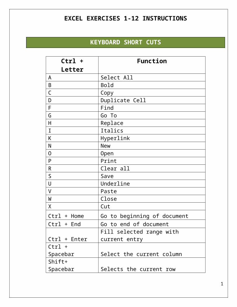
EXCEL EXERCISES 1-12 INSTRUCTIONS

KEYBOARD SHORT CUTS

Ctrl + Letter FunctionA Select AllB BoldC CopyD Duplicate CellF FindG Go ToH ReplaceI ItalicsK HyperlinkN NewO OpenP PrintR Clear allS SaveU UnderlineV PasteW CloseX Cut

Ctrl + Home Go to beginning of documentCtrl + End Go to end of document

Ctrl + Enter Fill selected range with current entryCtrl + Spacebar Select the current column

Shift+ Spacebar Selects the current row

Ctrl + 1 Display format cells dialog box

Ctrl + ` Displays Formulas (` is found next to #1)Ctrl + ; Enters date

1

Name Box

Exercise #1 – NAVIGATING &EXPLORING THE EXCEL WINDOW (IN-CLASS ACTIVITY)1. Open Excel.

2. Open the file Blue Sky Airlines.xlsx from the Excel Unit folder in the shared drive.

3. The purpose of this document is to familiarize yourself with Excel vocabulary as well as quick and easy methods of moving the cursor around a spreadsheet.

4. Click in cell H20 to make that cell active. Notice the cell reference appears in the Name Box.

5. Press the arrow key until B5 is selected. Notice the cell reference B5 appears in the Name Box.

6. Use the tab or arrow keys to move around the worksheet.

7. Use the Shift+Tab key combination to move one cell to the left.

8. Use the vertical scroll bar and buttons to move around the worksheet.

9. Drag the horizontal scroll box all the way to the right of the scroll bar.

10. Click on the Home tab. In the Editing group, select Find & Select, Go To.

11. Type B13 in the Reference text box. Click OK. The GoTo dialog box moves the active cell to B13. Notice B13 in the Name Box.

12. Press Ctrl + G to access the Go To dialog box again.

13. Use the Go To command to change the active cell to the following: AB90, BF305, G5

14. Click in the name box. Notice that G5 becomes highlighted.

15. Type D10 and thenpress the Enter key. Note that D10 is now the active cell (highlighted).

16. Choose all the different menus and notice the options in each menu.

17. Use the Close button to exit Excel. DO NOT SAVE.

2

IT IS VERY IMPORTANT THAT YOU SAVE YOUR WORK WITH THE FILENAME GIVEN TO YOU IN EACH EXERCISE! YOU WILL NOT DROP THE FILES TO ME UNTIL YOU ARE TOLD TO IN THE INSTRUCTIONS!

Exercise #2 – MAINDirections: Type the following worksheets in Excel. Save each exercise as a separate workbook as directed. You will open and add to these exercises again before dropping them to me.

1. Open Excel and a new blank workbook.

2. Save the workbookon your drive as MAIN.

3. Create the worksheet below. Do not enter any formulas in column C (Tax) or D (Total).

4. Resave and close the worksheet. Do NOTdrop it to me.

5. You will open MAIN and complete it in a later exercise.

3

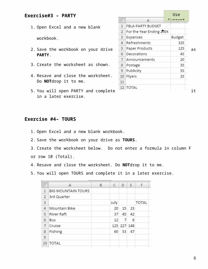
Exercise#3 – PARTY


2. Save the workbook on your drive as PARTY.

3. Create the worksheet as shown.

4. Resave and close the worksheet.Do NOTdrop it to me.

5. You will open PARTY and complete it in a later exercise.

Exercise #4– TOURS


2. Save the workbook on your drive as TOURS.

3. Create the worksheet below. Do not enter a formula in column F or row 10 (Total).

4. Resave and close the worksheet. Do NOTdrop it to me.

5. You will open TOURS and complete it in a later exercise.

4

Use CurrentYear

Exercise #5 – TICKET

1. Open Excel and a new blank workbook. Save the worksheet on your drive as TICKET.

2. Create the workbook below.

3. Enter a multiplication formula to calculate the Total in cell D5. Click in cell D5 and key the following formula: =B5*C5

4. Use the fill handle to copy the formula in cell D5 to cells D6, D7 and D8.HINT:Click in cell D5.Point the mouse to the bottom right corner of the cell. A solid black plus appears. This is the Fill Handle. Press the left mouse button and drag the Fill Handle down to copy the formula from D6 through D8.

5. Enter an additionformulain cell B10 to calculate the TOTALSin row 10. HINT: =B5+B6+B7+B8You may use the AutoSum, however this will be introduced in future lessons.

6. Use the fill handle to copy the formula in cell B10 to C10 and D10.

7. Resave as TICKET and close the worksheet. Do NOTdrop it to me.

8. You will open TICKET and complete it in a later exercise.

Exercise #6 -- PARTY

1. Open the PARTYworksheet that you completed in Exercise 3.

2. Change font size ofthe entire spreadsheet to 14 pt.

HINT: Select the entire spreadsheet and choose the Font group on the Home tab.

5

3. Key the Amount Spent title and values in column C as shown in the example on the last page.

4. Insert a blank row above row 3. (HINT:Click anywhere in row 3. Click Home tab, Cells group, InsertOR right-click, Insert, Entire RowOR right-click on the 3 and click Insert).

5. In cell D4 enter the label: Difference.

6. In cell D5, enter a formula to calculate the Difference in Column D. Difference is a subtraction formula. Use cell references. Some of the values will be negative because the amount spent was greater than the amount budgeted. HINT: =B5-C5

7. Use the fill handle to copy the formula in cell D5 to cells D6:D11.

8. Create an addition formula in B13. Include B12 in the cell range in case another expense is added to the list. HINT:UseAutoSum.

9. Use the fill handle to copy the addition formula in B13 to C13 and D13.

10. Center and bold all column headings in row 4.

11. Center the title in row 1 across columns A through D. HINT: Select A1:D1. Click on Merge & Center in the Alignment group on the Home tab. Center the title in row 2 the same way.

12. Create a border and shade light gray the titles in rows 1 and 2. HINT: Select A1:D2. Click on the down arrow of the Borders icon in the Font group on the Home Tab. Click on More Borders. Choose a style, click on the Outline button, and clickOK. Repeat the steps for light gray shading – shading is in the Fill tab.

13. Size all columns (AutoFit).HINT:Select the data. Home, Cells Group, Format, AutoFit Column Width. Make sure that all columns are font size 14.

14. Center the spreadsheet horizontally and vertically. HINT:Page Layout tab, Page Setup dialog box launcher (arrow in bottom right-hand corner), Margins tab.

15. Create a custom footer with your name, period, and Exercise Name: Exercise 6. HINT:Page Layout tab, Page Setup dialog box launcher, Header/Footer tab, Custom FooterOR Insert tab, Header & Footer, Go to Footer. Enter your information. Click out of the footer after you have enter your information.

16. Turn the gridlines on so they willappear on the worksheet when it is printed. HINT:Page Layout Tab, Sheet Options group, click on Print under Gridlines.

17. Do File, Print and look at the Preview of the document to make sure it looks correct. Do NOTdrop it to me.You will make changes to Exercise 6 in a later exercise.

18. Resave the spreadsheet as PARTY.

6

Exercise #7 – MAIN

1. Open the MAINworksheet that you completed in Exercise 2.

2. Change font on worksheet to 14 pt. HINT: Select the entire spreadsheet and choose Font Size from the Font group on the Home tab.

3. Insert an empty row above row 6.

4. If you have not done so already, key the current date in cell B3.HINT: Ctrl + ;

5. In cell C7 enter a formula to calculate a 5% TAX. Use either .05 or 5% in the formula. HINT: =B7*5%

6. Use the fill handle to copy the formula from C7 to C8:C13.

7. Enter a function to determine the TOTAL for Vitamins in cell D7. HINT: Add the sales and tax together by using the AutoSum() tool on the Home Tab, editing group.

8. Use the Fill Handle to copy the TOTAL formula for each department in column D.

9. Insert a row above the TOTAL SALES row.

10. Enter a function in cell B15 to calculate the TOTAL SALES. Use the AutoSum tool on the Home Tab.

11. Copy the TOTALS formula to cells C15 and D15.

12. Format the values in B7:C13 for Number and 2 decimal places. HINT:Select B7:C13. Click on the Home Tab, Number Group, click the down arrow next to General, select Number. If needed, click on the comma for larger numbers.

13. Format values in B15, C15, and D15 for Currency with 2 decimals. If any #### signs appear in the cells, size the column wider.HINT: Home tab, Number group, click the down arrow next to General, select Currency.

7

14. Format the totals values in D7-D13 for Currency with 2 decimals.

15. Center and bold the labels (text/words) in row 5.

16. Merge and Center the titles in row 1 and row 2 across columns. Remember you need to center each row separately.

17. Choose a border style and shade light gray cells A1:D2.

18. Size all columns (AutoFit). HINT: Home tab, Cells group, Format, AutoFit Column Width. Column A may have to be resized by dragging it smaller.

19. Center the worksheet vertically and horizontally on the page.

20. Create a custom footer with your name, period, and exercise nameExercise 7.

21. Click on File, Print and preview the spreadsheet. Make sure that gridlines are NOT showing. HINT:Page Layout tab, Sheet Options (only want check mark on View under Gridlines).

22. Copy the spreadsheet data to sheet 2. HINT: Select the entire spreadsheet. Ctrl C to Copy. Click on the + sign next to Sheet 1 to add Sheet 2.Click into A1 on Sheet 2. Ctrl V to Paste.

23. Show formulas. HINT: Formulas Tab, Formulas Auditing Group, Show formulasOR(Shortcut – CTRL `). When formulas are showing, some titles and dates may disappear. Don’t be concerned.Sheet 2 needs to show the formulas, not the titles.

24. Rename Sheet 2: Formulas 7. HINT: Double Click Sheet 2 tab.

25. If needed, size the columns so that all the formulas will appear (AutoFit).

26. Change the orientation to Landscape for Sheet 2 and make sure it fits on 1 page. HINT: Page Layout tab, Page Setup group, Orientation, Landscape. Page Layout tab, Scale to Fit group (change Width and Height to 1 page).

27. The footer from Sheet 1 did not copy onto Sheet 2. Create a custom footer with your name, period, and Formulas 7.

28. Turn on gridlines so they will print.

29. Center the spreadsheet horizontally and vertically.

30. Compare your worksheets to the answer key.

31. Save as: “P#-Lastname-Firstname-MAIN” and drop it to me.

Exercise #8 – TOURS

1. Open the TOURSworksheet that you completed in Exercise 4. Change the font to 14 pt.

8

2. AutoFit the columns.

3. Delete column B, the empty column. HINT:Click anywhere in column B, Right Click, Delete, Entire ColumnOR right-click on the B, Delete.

4. Insert a new, blank row above row 3.

5. Click into cell B4 – July. Use the Fill Handle to drag across C4 and D4 to create the months August and September.

6. In B11, AutoSum the July tours.

7. Use the Fill Handle to copy the AutoSum from B11 into C11, D11, and E11.

8. In E5, AutoSum the Mountain Bike figures for July through September.

9. Copy the AutoSum down through the other tours (E6:E9).

10. Type AVERAGE in cell A13.

11. Use the AVERAGE function to calculate the monthly averages in B13. (HINT:Formulas Tab, Insert function, ORfx on the formula barORthe down arrow on AutoSum. Argument = B5:B10—Never include totals in the average). Formula will look like: =AVERAGE(B5:B10). Use the Fill Handle to copy the function across to cells C13, D13, and E13.

12. Type MAXIMUM in cell A14.

13. Use the MAX function to calculate the monthly Maximum values in B14. (HINT: Formulas Tab, Insert function, ORfx on the formula bar ORthe down arrow on AutoSum. Argument = B5:B10—Never include totals in the maximum). Formula will look like: =MAX(B5:B10). Copy the function across to cells C14, D14, and E14.

14. Type MINIMUM in cell A15.

15. Use the MIN function to calculate the monthly Minimum values in B15. (HINT: Formulas Tab, Insert function, OR fx on the formula bar ORthe down arrow on AutoSum. Argument= B5:B10—Never include totals in the minimum). Formula will look like: =MIN(B5:B10). If MIN is not listed, type MIN in the Search for a Function box. Copy the function across to cells C15, D15, and E15.

16. Type COUNT in cell A16.

17. Use the COUNT NUMBERS function to calculate the monthly Counts in B16. (HINT: Formulas Tab, Insert function, ORfx on the formulas barORthe down arrow on AutoSum. Argument = B5:B10—Never include totals in the count). Formula will look like: =COUNT(B5:B10). Copy the function across to cells C16, D16, and E16.

9

18. Insert a new column to the left of column A. In A4 type: Tour No. To type numbers that are not to be calculated, type an apostrophe (‘) before the number. The apostrophe will left align the number. Excel will never use these numbers in a calculation or formula. Type the following data in the listed cells: A5 – ‘200, A6 – ‘300, A7 – ‘400, A8 – ‘500, A9 – ‘600.

19. Center and bold the title Tour Name in B4.

20. Follow the instructions below to sort rows 5-9 by the Tour Name column (column B) in ascending (A-Z) order.

Select A4 through F9. This includes all of the needed data in the sort. (If just one column of data is selected, Excel will sort just that column of information, mixing up the data across the rows.)

Home tab, Editing group, Sort & Filter Choose Custom Sort In the dialog box, choose:

o My data has headers (check box top right)o Choose Tour Name in the Sort by text boxo Choose Values in the Sort On text boxo Choose A to Z in the Order text boxo Click on OK

If sorted correctly, Bus with be at the top of the Tour Name column and 400 will be at the top of the Tour No. column.

21. Center and bold the column headings in row 4.

22. Shade light gray all the values in the TOTAL row and column.

23. Create a double line border around the AVERAGE, MAXIMUM, MINIMUM, and COUNT labels and values in rows 13 through 16.

24. Move the titles in rows 1 & 2 to cells A1 & A2. The titles will not center properly if they are typed in column B. Merge and Center the titles in rows 1 and 2across the columns.

25. AutoFit all columns. Drag column A if AutoFit makes the column too wide.


27. Create a custom footer with your name, period, and assignment name Exercise 8.

28. Insert an Online Pictureof your choice that is related to the spreadsheet. Size the graphic so that it fits below the spreadsheet data.HINT: Insert tab, Illustrations group, Online Pictures.

29. Take off gridlines so they do not print.

30. File, Print and preview the spreadsheet.

10

31. Copy the spreadsheet data to Sheet 2. Name Sheet 2: Formulas 8.

32. Show formulas. Show gridlines so they will print.

33. The footer from Sheet 1 did not copy onto sheet 2. Create a custom footer as done in above exercises.

34. Landscape and scale the spreadsheet to one page. Size the columns so that all the formulas appear.HINT: Page Layout tab, Page Setup group, Orientation, Landscape. Page Layout tab, Scale to Fit group (change Width and Height to 1 page).

35. Center the spreadsheet horizontally and vertically.

36. Compare your worksheets to the answer key.

37. Save as: “P#-Lastname-Firstname-TOURS” and drop it to me.

Exercise #9 – PARTY

1. Open the PARTYworksheet that you completed in Exercise 6. Change the font to 14 pt.

2. Cells B13:D13 should have been summed and the difference in Column D should have been calculated in Exercise 6. If not, turn back to Exercise 6 and follow the directions to AutoSum and calculate the difference now.

3. Move column D to column B. Columns B and C will become columns C and D.

a. Select column D by pointing to the D and then clicking on the green selector button at the top of column D. Hold the Shift button down; aim your mouse to the green border of column D. Get a four-headed move arrow. Drag column D to the left and next to column A. Let go of the Shift key. (Using the Shift key with the mouse automatically adds a new column and will not overwrite an existing column of data.)

11

The worksheet columns should look like the picture below.

4. Using Print Preview, check your border around cells A1:D2. Sometimes moving the columns moves the border as well. You may need to select cells A1:D2, turn off the border and then reapply the boarder again.


6. Use the AVERAGE function to calculate the average in cell B15. Copy across to cells C15 and D15.


8. Use the MAX function to calculate the Maximums in cell B16. Copy across to cells C16 and D16.

9. Type MINIMUM in cell A17.

10. Use the MIN function to calculate the Minimums in columns B17. Copy across to cells C17 and D17.


12. Use the COUNT NUMBERS function to calculate the Counts in cell B18. Copy Across to cells C18

and D18.

13. Sort rows 4-11 by the Expenses column in descending order. Select A4 through D11. HINT:Review instructions in Exercise 8 (Refreshments should appear in the Expenses column at the top of the column after the sort).

14. Center, bold, and italicize the column headings in row 4.

15. The titles in rows 1 and 2 should be merged and centered across columns A through D. Shade light gray and create a border around A1:D2.

12

16. Create a double line border around the AVERAGE, MAXIMUM, MINIMUM, and COUNT labels and values in rows 15 through 18.

17. Format the MAX, MIN, and COUNT values for number with no decimals.

18. Format the AVERAGE values for number and 1 decimal.

19. Insert an Office Picture of your choice that relates to the spreadsheet. Position the graphic below the spreadsheet data.

20. AutoFit the columns. Center the worksheet vertically and horizontally on the page.

21. Create a footer with your name, period, and Exercise 9.


23. Preview the spreadsheet.

24. Copy the spreadsheet data to Sheet 2. Name sheet 2: Formulas 9.

25. Show formulas.

26. Show gridlines so they will print.

27. Landscape the spreadsheet. Center the spreadsheet horizontally &vertically.

28. AutoFit the columns and make sure that it fits to one page.

29. The footer from Sheet 1 did not copy onto Sheet 2. Create a custom footer with your name, period, and Formulas 9.

30. Compare the worksheets to the answer key.

31. Save as: “P#-Lastname-Firstname-PARTY” and drop it to me.

Exercise 10 – TICKET

1. Open the TICKETworksheet that you completed in Exercise 5. Font-14 pt.


3. Select cell B12 and then use the COUNT NUMBERS function to calculate the rows B5 thru B8.

Use the Fill Handle to copy the Count from B12 into C12 and D12.


13

5. Select cell B13 and then use the MAX function to calculate the rows B5 thru B8. Use the Fill

Handle to copy the Maximum from B13 into C13 and D13.

6. Type MINIMUM in cell A14

7. Select cell B14 and then use the MIN function to calculate the rows B5 thru B8. Use the Fill

Handle to copy the Minimum from B14 into C14 and D14.


9. Select cell B15 and then use the AVERAGE function to calculate the rows B5 thru B8. Use the Fill

Handle to copy the Average from B15 into C15 and D15.

10. Format all values in cells B12:D15 for Number, with commas and no decimals.

11. Format all values in cells D5:D8 Total column for Currency and 2 decimals.

12. Format all values in C10:D10 for Currency and 2 decimals.

13. Format value in B10 for Number with comma and no decimals.

14. Merge and Center the titles in rows 1 and 2 across columns A through D.

15. Shade light gray and create a border around the titles in rows 1 & 2. Do not use the default single line for the border.

16. Center align and bold the column headings in row 4.

17. Insert a blank row below row 1. This will insert an empty row below the title: ROMEO & JULIET.

18. AutoFit all columns. Drag to size column A if the column is too wide.

19. Resave as TICKET and keep it open for the chart exercise.

14

Exercise 10 – CHARTUse the following information to create a CHART comparing the Type and the Total sales.Create the chart on the same page as the spreadsheet:

1. UsingTICKET, select only the data in the Type and Total Columns: A5:A9 and D5:D9. Use the Ctrl key to select nonadjacent cells. (Select A5:A9 first and then hold down the Ctrl key and select D5:D9).

2. Chart Type: 3-D Pie. HINT: Insert tab, Charts group, Pie, 3-D Pie.

3. Select Chart Layout 6HINT: Chart Tools tab, Design, Chart Layouts group, Quick Layouts.

4. Title: TICKET SALES, Font size 16 pt, bold.HINT: click inside the title on the chart and edit.

5. Subtitle: Romeo & Juliet, Font size 12 pt, bold.HINT: click at the end of the title and Enter.

6. Create a border of your choice around the title and subtitle. HINT: click on the title; Chart Tools tab, Format, Shape Styles group, Shape Outline, Automatic. Do it again and you can change the line weight and style.

7. Shade the title and subtitle light gray.HINT: click on the title; Chart Tools tab, Format, Shape Styles group, Shape Fill.

8. Create a border around the whole chart. Border style: Change the weight to 1 1/2 pt. Change the style to a dash type of your choice.HINT: click on the outside border and use Shape Outline in the Format contextual tab. Make sure you select Automatic for color.

9. Fill: Solid white

10. Move and size the chart so that it fits centered below the spreadsheet data. (Make sure the right border of the chart does not extend past the last column of the spreadsheet).


12. Click out of the chart into the spreadsheet. Create a custom footer with your name, period, and Exercise 10.



15. Copy Sheet 1 to Sheet 2 and show formulas.Name Sheet 2: Formulas 10. On Sheet 2, create a custom footer with your name, period, and Formulas 10.


17. Save as: “P#-Lastname-Firstname-TICKET” and drop it to me.

15

Exercise #11 – CHARTS

1. Open “P#-Lastname-Firstname-PARTY”. AutoFit the columns.2. DELETE THE DIFFERENCE COLUMN (COLUMN B).3. Use the following to create a CHART comparing the Budget and Amount Spent.

b. Select the data in cells A4:C11.

c. Create a column chart. Choose the clustered column subtype.

d. Chart Layout: Layout 9

e. Title—Font Size 18 pt., bold: FBLA PARTY

f. Subtitle—Font Size 12 pt., bold: Comparison of Budget and Amount Spent

g. Label X-Axis: Expenses

h. Label Y-Axis: Dollars

i. In the Design tab, Location group, click on Move Chart. Click on the New sheet button. Click on OK. (This puts the chart on a separate sheet with a tab named Chart1).

j. Change the bars for Amount Spent to display a fill of your choice. Choose a fill that can be easily seen.HINT: Right click on one of the Amount Spent bars, Format Data Series. Click on the Fill& Line bucket.

k. Create a 1 1/2 pt. dotted line border around the whole chart.

l. Create a solid line border of your choice around the title and subtitle.

m. Create a footer on the chart with your name, period, Exercise 11 – Party Chart.

4. Add Chart to the filename so Save as: “P#-Lastname-Firstname-PARTY CHART” and drop it to me.

CHART #2

1. Open the “P#-Lastname-Firstname-TOURS” file and create a chart.

2. Choose a different type of chart other than column or pie.Make sure that your chart makes sense. Determine what the chart is telling the reader and select what data you want in the chart. Insert the chart.

3. In the Design tab, Location group, click on Move Chart. Click on the New sheet button. Click on OK. (This puts the chart on a separate sheet with a tab named Chart1).

4. Choose a Layout and include a title, subtitle, borders, shading, etc.

5. Don’t forget to label the axis’s and make sure the legend is clearly labeled and clarifies the chart.

16

6. Create a footer on the chart with your name, period, Exercise 11 – Tours Chart.

7. Add Chart to the filename so Save as: “P#-Lastname-Firstname-TOURS CHART ” and drop it to me.

Exercise #12 – Real Estate – Review AssignmentSpreadsheet

1. Open EX12-Real Estate.xlsx from the Excel Unit folder in Shared drive.

2. In rows 1 & 2, change the font type and make the pt. size larger (you choose how large).

3. Merge and Center the titles in rows 1 &2 across columns A through D.

4. Bold and center the column headings.

5. Format the numbers with commas and no decimals.

6. Enter formulas in the Sales Change column to determine the difference between this month’s and last month’s sales. Use a subtraction formula (HINT:minus sign or hyphen). Some numbers will be in parenthesis which means they are a negative number.

7. Type the word TOTAL in all caps in cell A14.

8. Use the AutoSum function to calculate totals for the three money columns in row 14.

9. Type the word AVERAGE in all caps in cell A16.

10. Use the AVERAGE function to calculate averages in B16. Copy across.

11. Sort the spreadsheet in descending order by the Sales Change Column. Remember to select the data across the rows before sorting. Do NOT include the Totals or Averages in the sort. The Totals and Averages should remain at the bottom of the spreadsheet data. (Refer to Exercise 8 for instructions).

12. Create a dotted border and shade the totals and averages in A14 through D16.

13. Format the total row to Accounting Number Format with no decimals.HINT: click on the $ in the Number group and then Decrease Decimals.

14. Adjust the column widths to fit the text and numbers.

15. Center the spreadsheet vertically and horizontally on the page.

16. Create the standard class footer.Exercise 12

17. Take off gridlines so they do not print.

17


19. Copy the spreadsheet data to sheet 2. Name sheet 2: Formulas12.

20. Create a custom footer on Sheet 2 with your name, period, and Formulas 12.

21. Show formulas.

22. Show gridlines so they will print.

23. Landscape the spreadsheet.

24. Scale to Fit to one page. Horizontally and vertically center.


26. Save as: “P#-Lastname-Firstname-ANTELOPE SALES”. Do NOTdrop it to me. Keep it open for the chart below.

Chart Prepare a 2-D Pie Chartincluding the following:

1. Click on Sheet 1 to create the 2-D pie chart. Use Location and Last Month sales information from the spreadsheet. (Remember to use the Ctrl key to select nonadjacent cells. Select the Location column first and then hold down the Ctrl key and select the Last Month column).

2. Click on Move Chart in the Design tab, New Sheet, OK.

3. Include the title: ANTELOPE REAL ESTATE and the subtitle: SALES. Font size and style of your choice.

4. Choose an appropriate layout that includes pie slice percentages and a legend.

5. Create a border around the outside of the chart.

6. Explode the largest part of the pie.Hint: Left click until only that pie piece is selected. Right click on the pie piece, Format Data Point. In the right pane, change Point Explosion to 25%.

7. Create a standard class footer on the chart. Exercise 12 Chart.


9. Resave as: “P#-Lastname-Firstname-ANTELOPE SALES” and drop it to me.

18

Documents

DAILY Exercise -- #2munaco.weebly.com/.../excel_2013_ex_1 … · Web view · 2014-04-24Fill selected range with current entry. Ctrl + Spacebar . Select the current column