Damage Estimation and Localization from SparseAerial Imagery ∗

René García FranceschiniInstitute for Data, Systems and SocietyMassachusetts Institute of Technology

Cambridge, MAragarcia@mit.edu

Jeffrey LiuMIT Lincoln Laboratory

Lexington, MAJeffrey.Liu@ll.mit.edu

Saurabh AminDept. of Civil and Environmental Engineering

Massachusetts Institute of TechnologyCambridge, MAamins@mit.edu

Abstract

Aerial images provide important situational awareness for responding to naturaldisasters such as hurricanes. They are well-suited for providing information fordamage estimation and localization (DEL); i.e., characterizing the type and spatialextent of damage following a disaster. Despite recent advances in sensing andunmanned aerial systems technology, much of post-disaster aerial imagery isstill taken by handheld DSLR cameras from small, manned, fixed-wing aircraft.However, these handheld cameras lack IMU information, and images are takenopportunistically post-event by operators. As such, DEL from such imagery isstill a highly manual and time-consuming process. We propose an approach toboth detect damage in aerial images and localize it in world coordinates. Theapproach is based on using structure from motion to relate image coordinates toworld coordinates via a projective transformation, using class activation mapping todetect the extent of damage in an image, and applying the projective transformationto localize damage in world coordinates. We evaluate the performance of ourapproach on post-event data from the 2016 Louisiana floods, and find that ourapproach achieves a precision of 88%. Given this high precision using limited data,we argue that this approach is currently viable for fast and effective DEL fromhandheld aerial imagery for disaster response.

∗DISTRIBUTION STATEMENT A. Approved for public release. Distribution is unlimited.This material is based upon work supported by the United States Air Force under Air Force Contract No.

FA8702-15-D-0001. Any opinions, findings, conclusions or recommendations expressed in this material arethose of the author(s) and do not necessarily reflect the views of the United States Air Force.

© 2021 Massachusetts Institute of Technology.Delivered to the U.S. Government with Unlimited Rights, as defined in DFARS Part 252.227-7013 or 7014

(Feb 2014). Notwithstanding any copyright notice, U.S. Government rights in this work are defined by DFARS252.227-7013 or DFARS 252.227-7014 as detailed above. Use of this work other than as specifically authorizedby the U.S. Government may violate any copyrights that exist in this work.

This work was also made possible in part due to funding from NSF D-ISN project award # 2039771.

35th Conference on Neural Information Processing Systems (NeurIPS 2021), Sydney, Australia.

arX

iv:2

111.

0370

8v2

[ee

ss.I

V]

10

Nov

202

1

1 Application Context

Natural disasters, such as hurricanes and floods, can cause major loss of life and property; the intensity,scope, and the frequency of such disasters may be further exacerbated by global climate change [1].Timely information about the distribution and nature of damage following a disaster can help provideimportant context and information for emergency managers’ decision-making [2]. Increasingly,satellite and aerial imagery are being incorporated into post-disaster needs assessment [3]. However,while techniques exist for extracting information from orthorectified satellite and aerial imagery [4–8],methods for more general aerial imagery (such as oblique imagery from handheld cameras) havereceived far less attention. This is a critical limitation because post-disaster aerial imagery taken fromhandheld DSLR cameras from small, manned, fixed-wing aircraft remains popular due to the relativelylow cost, high availability, conformity with existing regulations, and existing training programsassociated with the practice [9, 10]. These handheld cameras lack IMU information, and imagesare taken opportunistically post-event by human operators, resulting in sparsely-sampled imagestaken at oblique angles. In this paper, we pose the question: how can we use aerial imagery froman arbitrary camera setup in order to rapidly and effectively aid in post-disaster situationalawareness?

We focus on a specific component of post-disaster needs assessment, which we refer to as DamageEstimation and Localization (DEL). We broadly define damage as an identifiable destruction of aninfrastructure component or utility resulting from a specific event (in our case, a natural disaster). Wethen define estimation as the detection of an instance of damage in an image. Finally, localization isthe act of assigning world coordinates to the estimated instance of damage. Our main contribution isa practically implementable approach that uses sparse, oblique aerial disaster imagery from handheldcameras to carry out DEL. To our knowledge, our approach is the only one that does estimationwithout relying on training data that includes bounding boxes or segmented images; and localizationwithout inertial measurement unit (IMU) information or a known geotransform. We show thatthis method applied to flooding DEL achieves a precision of 88% when compared against officialestimates from the 2016 Louisiana floods. We believe our approach provides emergency managersthe means to do fast and effective DEL using existing equipment.

The approach consists of two stages: a pre-disaster and a post-disaster stage. In the pre-disasterstage, a neural network is trained to classify damage within low altitude disaster imagery. Thepost-disaster stage is comprised of two parallel ’pipelines’, whose outputs are combined at the end.The first pipeline takes a collection of images from an area of interest and reconstructs the scene usingstructure from motion to obtain a projective transformation that relates image coordinates to worldcoordinates. The second pipeline takes individual images from the area of interest and producespolygons that cover the extent of the damage that is detected using class activation mapping. Theprojective transformation is then applied to the damage polygons to produce an estimate of damagelocations in world coordinates. Appendix A illustrates this approach.

Existing work in this area has focused primarily on nadir (top-down) or orthorectified imagery. Forgeoreferencing, common approaches use visual feature-based methods such as SIFT to registersatellite or nadir drone imagery to other known georeferenced images [11–14]. However, methodssuch as SIFT have been shown to perform poorly under extreme changes in perspective and sensorspecifications [13, 15]. Deep learning approaches using Siamese neural networks have been proposedfor georeferencing aerial images [15–18]; however, these approaches do not recover the orientationinformation necessary to project the oblique images to the world coordinates. Indeed, most availableliterature on registering oblique imagery relies on some variant of structure from motion or multiviewstereo [19], which is the approach we take for georeferencing. For detecting damage, various deeplearning approaches have achieved high accuracy in object detection challenges such as xView2 [4–6].Previous work has also attempted to overcome lack of training data in either satellite or aerial imagesvia transfer learning from satellite to aerial or vice versa [20–22]. Once again, these approaches wereonly applied to orthorectified imagery. Given the lack of tools and datasets developed for detectingdamage within oblique aerial photos, we pursue a weakly supervised approach to detecting damageusing class activation mapping.

2

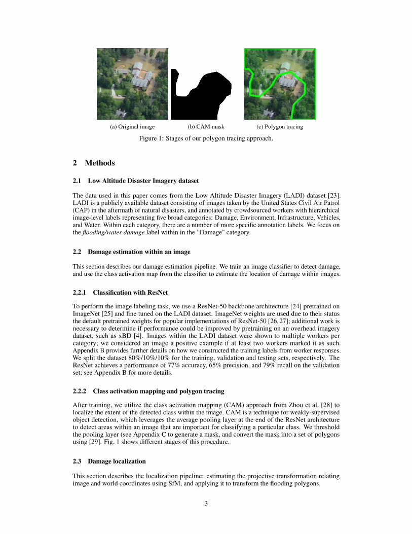
(a) Original image (b) CAM mask (c) Polygon tracing

Figure 1: Stages of our polygon tracing approach.

2 Methods

2.1 Low Altitude Disaster Imagery dataset

The data used in this paper comes from the Low Altitude Disaster Imagery (LADI) dataset [23].LADI is a publicly available dataset consisting of images taken by the United States Civil Air Patrol(CAP) in the aftermath of natural disasters, and annotated by crowdsourced workers with hierarchicalimage-level labels representing five broad categories: Damage, Environment, Infrastructure, Vehicles,and Water. Within each category, there are a number of more specific annotation labels. We focus onthe flooding/water damage label within in the “Damage" category.

2.2 Damage estimation within an image

This section describes our damage estimation pipeline. We train an image classifier to detect damage,and use the class activation map from the classifier to estimate the location of damage within images.

2.2.1 Classification with ResNet

To perform the image labeling task, we use a ResNet-50 backbone architecture [24] pretrained onImageNet [25] and fine tuned on the LADI dataset. ImageNet weights are used due to their statusthe default pretrained weights for popular implementations of ResNet-50 [26, 27]; additional work isnecessary to determine if performance could be improved by pretraining on an overhead imagerydataset, such as xBD [4]. Images within the LADI dataset were shown to multiple workers percategory; we considered an image a positive example if at least two workers marked it as such.Appendix B provides further details on how we constructed the training labels from worker responses.We split the dataset 80%/10%/10% for the training, validation and testing sets, respectively. TheResNet achieves a performance of 77% accuracy, 65% precision, and 79% recall on the validationset; see Appendix B for more details.

2.2.2 Class activation mapping and polygon tracing

After training, we utilize the class activation mapping (CAM) approach from Zhou et al. [28] tolocalize the extent of the detected class within the image. CAM is a technique for weakly-supervisedobject detection, which leverages the average pooling layer at the end of the ResNet architectureto detect areas within an image that are important for classifying a particular class. We thresholdthe pooling layer (see Appendix C to generate a mask, and convert the mask into a set of polygonsusing [29]. Fig. 1 shows different stages of this procedure.

2.3 Damage localization

This section describes the localization pipeline: estimating the projective transformation relatingimage and world coordinates using SfM, and applying it to transform the flooding polygons.

3

2.3.1 Reconstruction using structure from motion

Structure from motion is a technique that, using images from a camera moving through an environ-ment, can produce a point cloud of the environment [30]. By taking advantage of the GPS tags fromthe image metadata or from outside sensors, structure from motion has been used to create inexpen-sive, georeferenced elevation models from drone and aircraft imagery [31]. We use this techniqueas an intermediate step to obtaining the projective transformation that relates image coordinates toworld coordinates. We base our implementation off the well-known OpenSfM library, an open sourcelibrary for structure from motion [32].

Since fixed wing aircraft tend to fly in a straight line, and have a relatively large turn radius compared torotary-wing aircraft, sequential images collected from fixed-wing platforms tend to be approximatelycollinear. Thus, some reconstructions have an additional degree of freedom from rotating about theline that goes through the GPS coordinates. We address this by separately estimating the directionof the up-vector (the vector opposite the direction of gravity) and enforcing it in the reconstruction.Previous implementations in urban environments have suggested estimating vanishing points toestimate the up-vector [33]. This may be difficult if there are few straight features (such as roads),which is common in rural areas.

To estimate the up-vector, we assume the ground is approximately flat. We first fit a plane throughthe reconstructed features using RANSAC [34]. There is a pair of possible antiparallel unit normalvectors to this plane, one of which is the up-vector. Because of the aerial nature of the data, thelocation of the images must be above the ground plane. Therefore, we choose the vector that hasa positive projection onto the image location in East, North Up (ENU) coordinates and denote itvup. Finally, we rotate the reconstruction so that vup indeed points upwards. Specifically, we rotateit by Rz such that Rzvup = z when it is initialized, and the up-vector is enforced during bundleadjustment. In areas with significant variation in local topology, a digital elevation model (DEM)can be used to estimate the ground plane. We had initially incorporated a digital elevation model(DEM). However, since the region that we considered is relatively flat, there was no difference inperformance, and thus, we do not report the DEM results.

2.3.2 Image-to-world projective transformation

The final step in our georeferencing pipeline is estimating the transformation from image coordinatesto world coordinates, and applying it to the detected damage polygons. As discussed previously,the images are of mostly flat surfaces, and thus the coordinates can be related by a projectivetransformation [30], and outliers can be filtered through RANSAC [34]. Of all of the images thatwere reconstructed using OpenSfM, we retained those where at least 20% of matches between imageand world coordinates were inliers. Of the retained images, we found that some images producedextremely large image footprints (i.e., , the projection of the image edges onto the ground). Weidentified that these photos were those that were so oblique that the horizon was visible. Because suchimages require more complex transformations, we eliminated them from our analysis. We consideredtwo heuristic criteria for eliminating such images. First, we eliminated images whose total area weregreater than some value γ1. Second, we did not consider images where the ratio of the longest sideto the shortest side of the minimum area rectangle that covered the entire footprint was greater thanγ2. We report our results for a variety of γ1 and γ2 parameters to illustrate the effectiveness of ourapproach.

3 Evaluation and Results

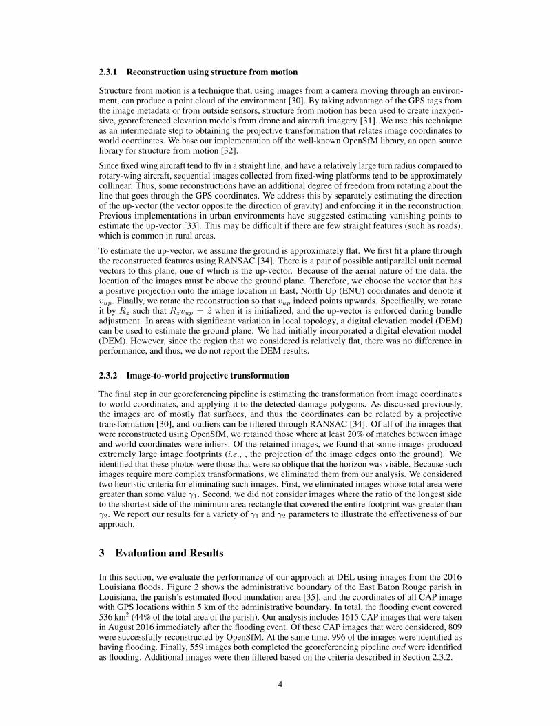
In this section, we evaluate the performance of our approach at DEL using images from the 2016Louisiana floods. Figure 2 shows the administrative boundary of the East Baton Rouge parish inLouisiana, the parish’s estimated flood inundation area [35], and the coordinates of all CAP imagewith GPS locations within 5 km of the administrative boundary. In total, the flooding event covered536 km2 (44% of the total area of the parish). Our analysis includes 1615 CAP images that were takenin August 2016 immediately after the flooding event. Of these CAP images that were considered, 809were successfully reconstructed by OpenSfM. At the same time, 996 of the images were identified ashaving flooding. Finally, 559 images both completed the georeferencing pipeline and were identifiedas flooding. Additional images were then filtered based on the criteria described in Section 2.3.2.

4

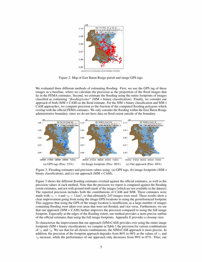
Figure 2: Map of East Baton Rouge parish and image GPS tags.

We evaluated three different methods of estimating flooding. First, we use the GPS tag of theseimages as a baseline, where we calculate the precision as the proportion of the flood images thatlie in the FEMA estimates. Second, we estimate the flooding using the entire footprints of imagesclassified as containing “flooding/water" (SfM + binary classification). Finally, we consider ourapproach of both (SfM + CAM) as the flood estimate. For the SfM + binary classification and SfM +CAM approaches, we compute precision as the fraction of the computed flooding polygons whichoverlap with the official FEMA estimates. We only consider the flooding within the East Baton Rougeadministrative boundary, since we do not have data on flood extent outside of the boundary.

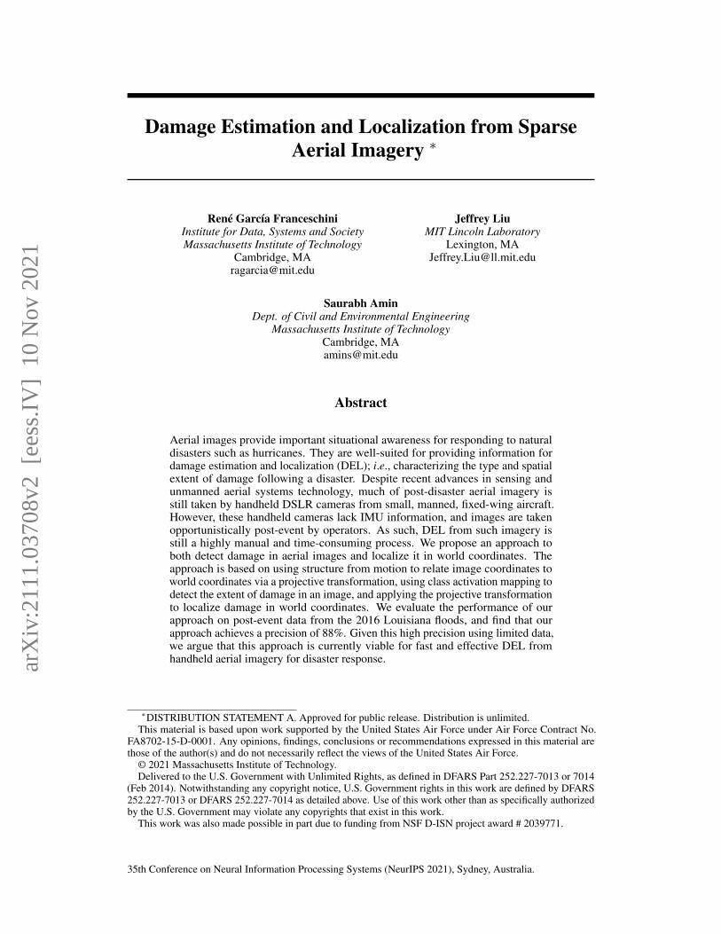
(a) GPS tags (Prec: 52%) (b) Image footprints (Prec: 80%) (c) Our approach (Prec: 88%)

Figure 3: Flooding estimates and precision values using: (a) GPS tags, (b) image footprints (SfM +binary classification), and (c) our approach (SfM + CAM).

Figure 3 shows the different flooding estimates overlaid against the official estimates, as well as theprecision values of each method. Note that the precision we report is compared against the floodingextent estimates, and not with ground truth mask of the images (which are not available in the dataset).The reported precision includes both the contributions of CAM and SfM. These estimates weremade with γ1 = 4 and γ2 = 5 km2, so that ultimately 243 images were used. These results show aclear improvement going from using the image GPS locations to using the georeferenced footprint.This suggests that using the GPS of the image location is insufficient, as a large number of imagescontaining flooding were taken over areas that were not flooded, and vice versa. Furthermore, we seethat our approach (SfM + CAM) further improves the precision compared to using the full imagefootprint. Especially at the edges of the flooding extent, our method provides a more precise outlineof the official estimates than using the full image footprints. Appendix E provides a closeup view.

To characterize the improvement that our approach (SfM+CAM) provides over using the entire imagefootprints (SfM + binary classification), we compute in Table 1 the precision for various combinationsof γ1 and γ2. We see that for all chosen combinations, the SfM+CAM approach is more precise. Inaddition, the precision of the footprint approach degrades from 86% to 68% as the values of γ1 andγ2 increase, while the performance of our approach only decreases from 90% to 87%. Thus, our

5

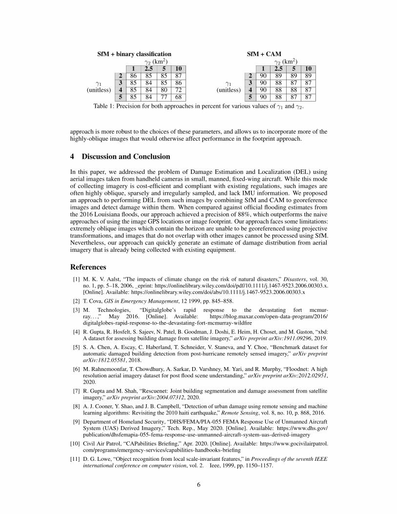
SfM + binary classificationγ2 (km2)

1 2.5 5 102 86 85 85 873 85 84 85 864 85 84 80 72

γ1(unitless)

5 85 84 77 68

SfM + CAMγ2 (km2)

1 2.5 5 102 90 89 89 893 90 88 87 874 90 88 88 87

γ1(unitless)

5 90 88 87 87Table 1: Precision for both approaches in percent for various values of γ1 and γ2.

approach is more robust to the choices of these parameters, and allows us to incorporate more of thehighly-oblique images that would otherwise affect performance in the footprint approach.

4 Discussion and Conclusion

In this paper, we addressed the problem of Damage Estimation and Localization (DEL) usingaerial images taken from handheld cameras in small, manned, fixed-wing aircraft. While this modeof collecting imagery is cost-efficient and compliant with existing regulations, such images areoften highly oblique, sparsely and irregularly sampled, and lack IMU information. We proposedan approach to performing DEL from such images by combining SfM and CAM to georeferenceimages and detect damage within them. When compared against official flooding estimates fromthe 2016 Louisiana floods, our approach achieved a precision of 88%, which outperforms the naiveapproaches of using the image GPS locations or image footprint. Our approach faces some limitations:extremely oblique images which contain the horizon are unable to be georeferenced using projectivetransformations, and images that do not overlap with other images cannot be processed using SfM.Nevertheless, our approach can quickly generate an estimate of damage distribution from aerialimagery that is already being collected with existing equipment.

References[1] M. K. V. Aalst, “The impacts of climate change on the risk of natural disasters,” Disasters, vol. 30,

no. 1, pp. 5–18, 2006, _eprint: https://onlinelibrary.wiley.com/doi/pdf/10.1111/j.1467-9523.2006.00303.x.[Online]. Available: https://onlinelibrary.wiley.com/doi/abs/10.1111/j.1467-9523.2006.00303.x

[2] T. Cova, GIS in Emergency Management, 12 1999, pp. 845–858.

[3] M. Technologies, “Digitalglobe’s rapid response to the devastating fort mcmur-ray. . . ,” May 2016. [Online]. Available: https://blog.maxar.com/open-data-program/2016/digitalglobes-rapid-response-to-the-devastating-fort-mcmurray-wildfire

[4] R. Gupta, R. Hosfelt, S. Sajeev, N. Patel, B. Goodman, J. Doshi, E. Heim, H. Choset, and M. Gaston, “xbd:A dataset for assessing building damage from satellite imagery,” arXiv preprint arXiv:1911.09296, 2019.

[5] S. A. Chen, A. Escay, C. Haberland, T. Schneider, V. Staneva, and Y. Choe, “Benchmark dataset forautomatic damaged building detection from post-hurricane remotely sensed imagery,” arXiv preprintarXiv:1812.05581, 2018.

[6] M. Rahnemoonfar, T. Chowdhury, A. Sarkar, D. Varshney, M. Yari, and R. Murphy, “Floodnet: A highresolution aerial imagery dataset for post flood scene understanding,” arXiv preprint arXiv:2012.02951,2020.

[7] R. Gupta and M. Shah, “Rescuenet: Joint building segmentation and damage assessment from satelliteimagery,” arXiv preprint arXiv:2004.07312, 2020.

[8] A. J. Cooner, Y. Shao, and J. B. Campbell, “Detection of urban damage using remote sensing and machinelearning algorithms: Revisiting the 2010 haiti earthquake,” Remote Sensing, vol. 8, no. 10, p. 868, 2016.

[9] Department of Homeland Security, “DHS/FEMA/PIA-055 FEMA Response Use of Unmanned AircraftSystem (UAS) Derived Imagery,” Tech. Rep., May 2020. [Online]. Available: https://www.dhs.gov/publication/dhsfemapia-055-fema-response-use-unmanned-aircraft-system-uas-derived-imagery

[10] Civil Air Patrol, “CAPabilities Briefing,” Apr. 2020. [Online]. Available: https://www.gocivilairpatrol.com/programs/emergency-services/capabilities-handbooks-briefing

[11] D. G. Lowe, “Object recognition from local scale-invariant features,” in Proceedings of the seventh IEEEinternational conference on computer vision, vol. 2. Ieee, 1999, pp. 1150–1157.

6

[12] J. Oh, C. K. Toth, and D. A. Grejner-Brzezinska, “Automatic georeferencing of aerial images using stereohigh-resolution satellite images,” Photogrammetric Engineering & Remote Sensing, vol. 77, no. 11, pp.1157–1168, 2011.

[13] X. Zhuo, T. Koch, F. Kurz, F. Fraundorfer, and P. Reinartz, “Automatic uav image geo-registration bymatching uav images to georeferenced image data,” Remote Sensing, vol. 9, no. 4, p. 376, 2017.

[14] H. Goncalves, L. Corte-Real, and J. A. Goncalves, “Automatic image registration through image segmenta-tion and sift,” IEEE Transactions on Geoscience and Remote Sensing, vol. 49, no. 7, p. 2589–2600, Jul2011.

[15] A. Shetty and G. X. Gao, “Uav pose estimation using cross-view geolocalization with satellite imagery,” in2019 International Conference on Robotics and Automation (ICRA). IEEE, 2019, pp. 1827–1833.

[16] Y. Tian, C. Chen, and M. Shah, “Cross-view image matching for geo-localization in urban environments,”in Proceedings of the IEEE Conference on Computer Vision and Pattern Recognition, 2017, pp. 3608–3616.

[17] D.-K. Kim and M. R. Walter, “Satellite image-based localization via learned embeddings,” in 2017 IEEEInternational Conference on Robotics and Automation (ICRA). IEEE, 2017, pp. 2073–2080.

[18] L. Liu and H. Li, “Lending orientation to neural networks for cross-view geo-localization,” in Proceedingsof the IEEE/CVF Conference on Computer Vision and Pattern Recognition, 2019, pp. 5624–5633.

[19] S. Verykokou and C. Ioannidis, “Oblique aerial images: a review focusing on georeferencing procedures,”International Journal of Remote Sensing, vol. 39, no. 11, pp. 3452–3496, 2018.

[20] L. Cao, C. Wang, and J. Li, “Vehicle detection from highway satellite images via transfer learning,”Information sciences, vol. 366, pp. 177–187, 2016.

[21] Y. Liang, S. T. Monteiro, and E. S. Saber, “Transfer learning for high resolution aerial image classification,”in 2016 IEEE Applied Imagery Pattern Recognition Workshop (AIPR). IEEE, 2016, pp. 1–8.

[22] S. Ji, S. Wei, and M. Lu, “A scale robust convolutional neural network for automatic building extractionfrom aerial and satellite imagery,” International journal of remote sensing, vol. 40, no. 9, pp. 3308–3322,2019.

[23] J. Liu, D. Strohschein, S. Samsi, and A. Weinert, “Large scale organization and inference of an imagerydataset for public safety,” in 2019 IEEE High Performance Extreme Computing Conference (HPEC), Sep.2019, pp. 1–6.

[24] K. He, X. Zhang, S. Ren, and J. Sun, “Deep residual learning for image recognition,” in Proceedings of theIEEE conference on computer vision and pattern recognition, 2016, pp. 770–778.

[25] J. Deng, W. Dong, R. Socher, L.-J. Li, K. Li, and L. Fei-Fei, “Imagenet: A large-scale hierarchical imagedatabase,” in 2009 IEEE conference on computer vision and pattern recognition. Ieee, 2009, pp. 248–255.

[26] K. Team, “Keras documentation: ResNet and ResNetV2.” [Online]. Available: https://keras.io/api/applications/resnet/#resnet50-function

[27] “torchvision.models — Torchvision 0.11.0 documentation.” [Online]. Available: https://pytorch.org/vision/stable/models.html

[28] B. Zhou, A. Khosla, A. Lapedriza, A. Oliva, and A. Torralba, “Learning deep features for discriminativelocalization,” in Proceedings of the IEEE conference on computer vision and pattern recognition, 2016, pp.2921–2929.

[29] S. Suzuki et al., “Topological structural analysis of digitized binary images by border following,” Computervision, graphics, and image processing, vol. 30, no. 1, pp. 32–46, 1985.

[30] A. M. Andrew, “Multiple view geometry in computer vision,” Kybernetes, 2001.

[31] M. A. Fonstad, J. T. Dietrich, B. C. Courville, J. L. Jensen, and P. E. Carbonneau, “Topographic struc-ture from motion: a new development in photogrammetric measurement,” Earth surface processes andLandforms, vol. 38, no. 4, pp. 421–430, 2013.

[32] mapillary, “Opensfm,” https://github.com/mapillary/OpenSfM, Feb 2021. [Online]. Available:https://github.com/mapillary/OpenSfM

[33] C.-P. Wang, K. Wilson, and N. Snavely, “Accurate georegistration of point clouds using geographic data,”in 2013 International Conference on 3D Vision-3DV 2013. IEEE, 2013, pp. 33–40.

[34] M. A. Fischler and R. C. Bolles, “Random sample consensus: a paradigm for model fitting with applicationsto image analysis and automated cartography,” Communications of the ACM, vol. 24, no. 6, pp. 381–395,1981.

[35] C. of Baton Rouge and P. of East Baton Rouge, “The great flood of 2016 story map,” https://ebrgis.maps.arcgis.com/apps/MapSeries/index.html?appid=1c4ac\9fca97846d2a1780a90fc68c6eb, Aug2016. [Online]. Available: https://ebrgis.maps.arcgis.com/apps/MapSeries/index.html?appid=1c4ac\9fca97846d2a1780a90fc68c6eb

7

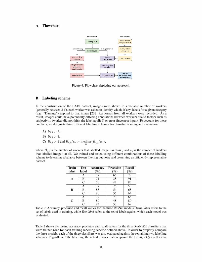
A Flowchart

Figure 4: Flowchart depicting our approach.

B Labeling scheme

In the construction of the LADI dataset, images were shown to a variable number of workers(generally between 3-5); each worker was asked to identify which, if any, labels for a given category(e.g. “Damage") applied to that image [23]. Responses from all workers were recorded. As aresult, images could have potentially differing annotations between workers due to factors such assubjectivity (worker did not think the label applied) or error (incorrect input). To account for theseconflicts, we designate three different labelling schemes for classifier training and evaluation:

A) Bi,j > 1,

B) Bi,j > 2,

C) Bi,j > 1 and Bi,j/wi > median∀i{Bi,j/wi},

where Bi,j is the number of workers that labelled image i as class j and wi is the number of workersthat labelled image i at all. We trained and tested using different combinations of these labellingscheme to determine a balance between filtering out noise and preserving a sufficiently representativedataset.

Trainlabel

Testlabel

Accuracy(%)

Precision(%)

Recall(%)

AA 77 65 79B 71 38 91C 70 42 83

BA 77 75 53B 83 54 68C 80 55 64

CA 79 73 65B 80 48 80C 83 53 69

Table 2: Accuracy, precision and recall values for the three ResNet models. Train label refers to theset of labels used in training, while Test label refers to the set of labels against which each model wasevaluated.

Table 2 shows the testing accuracy, precision and recall values for the three ResNet50 classifiers thatwere trained (one for each training labelling scheme defined above. In order to properly comparethe three models, each of the three classifiers was also evaluated against the remaining two labellingschemes. Regardless of the labelling, the actual images that comprised the testing set (as well as the

8

training and validation sets) were the same for all three schemes. For the purposes of this paper, wewill refer to each of the models according to their training labelling scheme.

Unsurprisingly, each of three models had the highest accuracy when compared against the labellingscheme they were trained on. With the other two metrics, though, there are noticeable trends. Interms of precision, model B had the highest precision when evaluated against any labelling scheme,followed by C and finally A. With recall, the opposite holds: A has the highest recall across the board,followed by C and then B. These trends are not difficult to justify, since B necessarily has a higherstandard for classification as flooding than A. For flooding, C is a compromise between the mostlenient labelling scheme (A) and the strictest one (C). In this particular application, we consider falsepositives to be less serious than false negatives; that is, we would rather think that someone was indanger from flooding when they are not (false positive) than think that they are not in danger whenthey are (false negative). As such, we proceed using model A for the remainder of the section.

C CAM details

Using the terminology in [28], the output on the final fully connected layer is given by:

Sc =∑k

wck

∑x,y

fk(x, y) =∑x,y

∑k

wckfk(x, y), (1)

where wck is the weight corresponding to class c for the k-th unit within conv5 (the final block

within ResNet-50) and fk(x, y) is the activation of the same k-th unit at location (x, y) (such that∑x,y fk(x, y) is the output of the global pooling layer). Let Mc(x, y) =

∑k w

ckfk(x, y), so that:

Sc =∑x,y

Mc(x, y). (2)

Here, Mc(x, y) can be viewed as a measure of importance of a spatial coordinate (x, y) for the classc = flooding/water damage, and hence referred to the class activation map. In order to determine theboundaries of the flooding instances, we threshold on Mc:

Mmaskc (x, y) =

{1 if Mc(x, y) ≥ 0

0 otherwise(3)

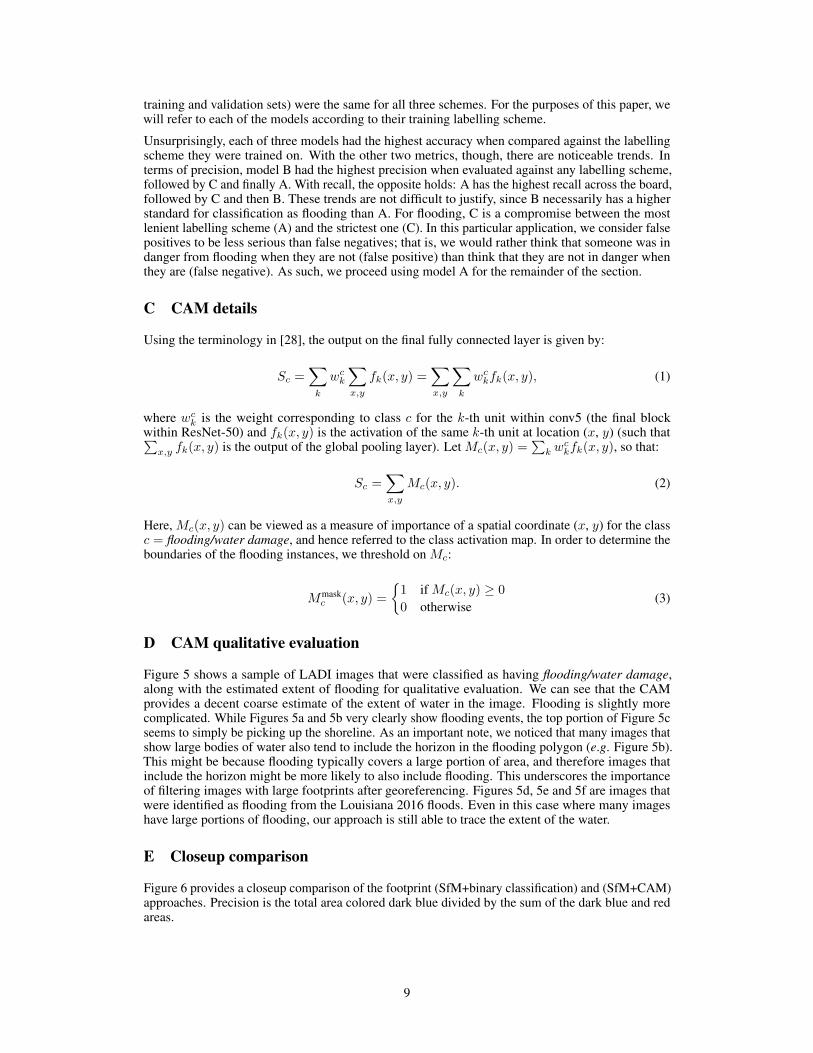
D CAM qualitative evaluation

Figure 5 shows a sample of LADI images that were classified as having flooding/water damage,along with the estimated extent of flooding for qualitative evaluation. We can see that the CAMprovides a decent coarse estimate of the extent of water in the image. Flooding is slightly morecomplicated. While Figures 5a and 5b very clearly show flooding events, the top portion of Figure 5cseems to simply be picking up the shoreline. As an important note, we noticed that many images thatshow large bodies of water also tend to include the horizon in the flooding polygon (e.g. Figure 5b).This might be because flooding typically covers a large portion of area, and therefore images thatinclude the horizon might be more likely to also include flooding. This underscores the importanceof filtering images with large footprints after georeferencing. Figures 5d, 5e and 5f are images thatwere identified as flooding from the Louisiana 2016 floods. Even in this case where many imageshave large portions of flooding, our approach is still able to trace the extent of the water.

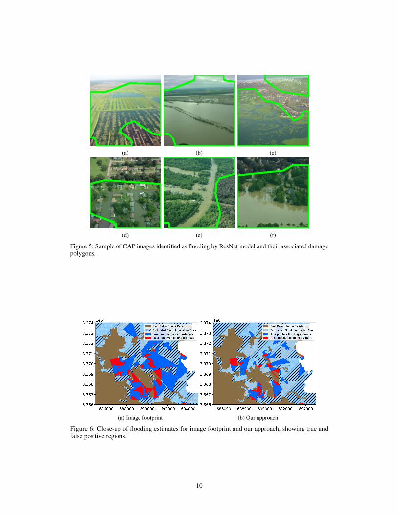
E Closeup comparison

Figure 6 provides a closeup comparison of the footprint (SfM+binary classification) and (SfM+CAM)approaches. Precision is the total area colored dark blue divided by the sum of the dark blue and redareas.

9

(a) (b) (c)

(d) (e) (f)

Figure 5: Sample of CAP images identified as flooding by ResNet model and their associated damagepolygons.

(a) Image footprint (b) Our approach

Figure 6: Close-up of flooding estimates for image footprint and our approach, showing true andfalse positive regions.

10