Dan Gillen Department of Statistics University of ...dgillen/STAT255/Handouts/lecture4.pdfI Equivalent to the Wilcoxon rank sum statistic when there is no censoring. I The Gˆ; family

Lecture 4

Stat 255 - D. Gillen

Weighted LogrankTests

K -Sample LogrankTests

K -Sample (Tarone)Test for Trend

Stratified LogrankTestsMatched Tests

Summary

4.1

Lecture 4

Extensions of the Logrank TestStatistics 255 - Survival Analysis

Presented January 21, 2016

Dan GillenDepartment of Statistics

University of California, Irvine

Lecture 4






Summary

4.2

Weighted Logrank Tests

Logrank and Mantel-Haenzel Test

M-H Test Series of (independent) tables at different levels ofa confounder C

I Data at level C = k :D D

E ak bk

E ck dk

I M-H test compares Pr[D|E,C = k ] and Pr[D|E,C = k ] andis designed (most powerful) for the case where the oddsratio, ψk is constant at all levels of C:

ψk =Pr[D|E,C = k ]/Pr[D|E,C = k ]

Pr[D|E,C = k ]/Pr[D|E,C = k ]

Lecture 4






Summary

4.3


Logrank and Mantel-Haenzel Test

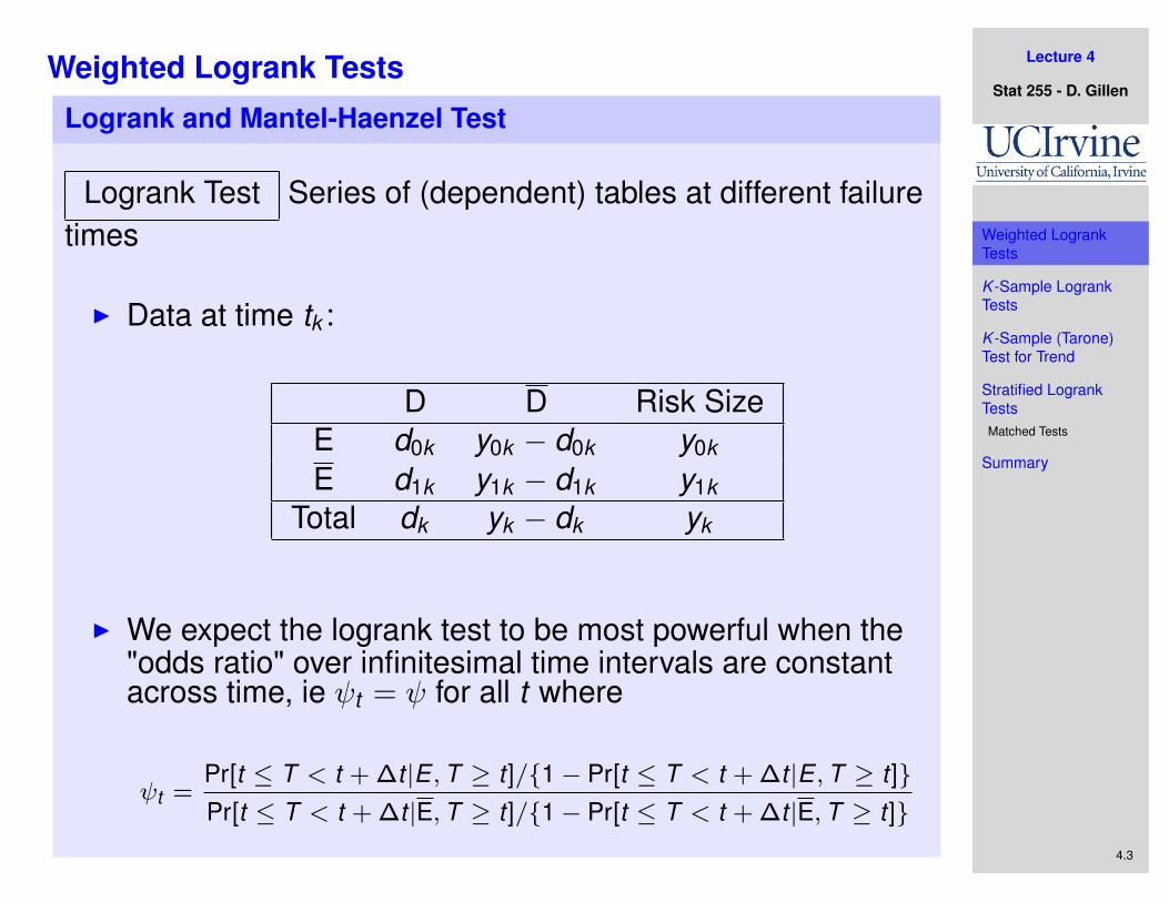
Logrank Test Series of (dependent) tables at different failuretimes

I Data at time tk :

D D Risk SizeE d0k y0k − d0k y0k

E d1k y1k − d1k y1k

Total dk yk − dk yk

I We expect the logrank test to be most powerful when the"odds ratio" over infinitesimal time intervals are constantacross time, ie ψt = ψ for all t where

ψt =Pr[t ≤ T < t + ∆t |E ,T ≥ t]/{1− Pr[t ≤ T < t + ∆t |E ,T ≥ t]}Pr[t ≤ T < t + ∆t |E,T ≥ t]/{1− Pr[t ≤ T < t + ∆t |E,T ≥ t]}

Lecture 4






Summary

4.4


Proportional Hazards

I But, as ∆t ↓ 0I 1− Pr’s ↑ 1I Ratio of Pr’s→ ratio of hazards, ie

ψt ≈λ(t |E)

λ(t |E)

I The logrank test will be most powerful for the case wherethe hazard ratio remains constant over time. This is calledthe proportional hazards case.

Lecture 4






Summary

4.5


Ex. Proportional Hazards

Time (months)

Surv

ival

0 10 20 30

0.0

0.2

0.4

0.6

0.8

1.0

Control ~ Exponential (.050)Treatment ~ Exponential( .050/1.56 )

Lecture 4






Summary

4.6


Ex. Non-Proportional Hazards

Time (months)

Surv

ival

0 10 20 30

0.0

0.2

0.4

0.6

0.8

1.0

Control ~ Weibull(1.5,16.9)Treatment ~ Weibull (.90,31.3)

Lecture 4






Summary

4.7


Weighted Logrank Statistics

I Consider weighting (Obs − Exp) differently over time

I This will enable us to inflate early or late differences

→ Potential for increased power under non-proportionalhazards

TW =

[∑Dk=1 wk (Ok − Ek )

]2

∑Dk=1 w2

k Vk=

[∑Dk=1 wk Uk

]2

∑Dk=1 w2

k Vk

Lecture 4






Summary

4.8


Weighted Logrank Statistics

I Choices for wk that have been proposed:

1. wk = nk gives the Gehan-Breslow test (weights equal tothe total number of subjects at risk at each failure time).Applies greater weight to early failure times.

2. wk = SKM (tk−) gives the generalized Wilcoxon test(weights equal to the pooled estimate of survival just prior totime tk ). Applies greater weight to early failure times.

I Equivalent to the Wilcoxon rank sum statistic when there is nocensoring.

I The Gρ,γ family (Fleming and Harrington; 1991)

I wk =[SKM (tk−)

]ρ [1− SKM (tk−)

]γI ρ = γ = 0 gives the usual logrank statisticI ρ = 1 and γ = 0 gives the generalized Wilcoxon test

Lecture 4






Summary

4.9


Power Comparisons - Proportional Hazards

Time

Surv

ival

0.0

0.2

0.4

0.6

0.8

1.0

0 1 2 3 4

Hazard Ratio Over Time(Cox estimate: 0.50)

HR = 1/2

Theta

Pow

er

1.0 1.5 2.0 2.5 3.0

0.2

0.4

0.6

0.8

1.0

Rho=0, Gamma=0 (Logrank)Rho=1, Gamma=0 (Wilcoxon)Rho=0, Gamma=1Rho=1, Gamma=1

Lecture 4






Summary

4.10


Power Comparisons - Early Diverging Hazards

Time

Surv

ival

0.0

0.2

0.4

0.6

0.8

1.0

0 1 2 3 4


HR = 1/2 HR = 2 HR = 1

Pow

er

1.0 1.1 1.2 1.3 1.4 1.5

0.2

0.4

0.6

0.8

1.0


Lecture 4






Summary

4.11


Power Comparisons - Late Diverging Hazards

Time

Surv

ival

0.0

0.2

0.4

0.6

0.8

1.0

0 1 2 3 4


HR = 1 HR = 1/2

Pow

er

1.0 1.2 1.4 1.6 1.8

0.2

0.4

0.6

0.8

1.0


Lecture 4






Summary

4.12


Implementation in R - 6MP Example

I Know that the (unweighted) logrank statistic will be mostpowerful under proportional hazards

I How can we (informally) check the proportional hazardsassumption?

I If we have proportional hazards, then

λ1(t) = φλ0(t)

so that

log Λ1(t) = log(φ) + log Λ0(t)

I So, if the log cumulative hazards are roughly parallel, thelogrank test will tend to be most powerful

Lecture 4






Summary

4.13


6MP log-Cumulative Hazards Plot

plot( survfit( Surv( time, irelapse ) ~ sixmp, data=sixmpLong ),fun="cloglog", lty=1:2, mark.time=FALSE,xlab="Time (mths)", ylab="log-Cumulative Hazard" )

legend( 1,1, lty=1:2, legend=c("Control (N=21)", "6-MP (N=21)"),bty="n" )

1 2 5 10 20

−2.

0−

1.5

−1.

0−

0.5

0.0

0.5

1.0

Time (mths)

log−

Cum

ulat

ive

Haz

ard

Control (N=21)6−MP (N=21)

Lecture 4






Summary

4.14


Implementation in R - 6MP Example

I Not too bad...We do not expect the generalized Wilcoxontest to be as powerful as the logrank test in this situation

I To compute the generalized Wilcoxon, specify the optionrho=1 in the survdiff() function

I Note: The Gρ,γ statistic is not currently implemented in thesurvival package

> ##### Usual (unweight LR test)> survdiff( Surv( time, irelapse ) ~ sixmp, rho=0, data=sixmpLong )

N Observed Expected (O-E)^2/E (O-E)^2/Vsixmp=0 21 21 10.7 9.77 16.8sixmp=1 21 9 19.3 5.46 16.8

Chisq= 16.8 on 1 degrees of freedom, p= 4.17e-05

> ##### Generalized Wilcoxon test> survdiff( Surv( time, irelapse ) ~ sixmp, rho=1, data=sixmpLong )

N Observed Expected (O-E)^2/E (O-E)^2/Vsixmp=0 21 14.55 7.68 6.16 14.5sixmp=1 21 5.12 12.00 3.94 14.5

Chisq= 14.5 on 1 degrees of freedom, p= 0.000143

Lecture 4






Summary

4.15


How should weights be chosen?

I For scientific inference it is not reasonable to look at thesurvival curves first, then choose weights

I First, ask whether there is a reason to believe we will havenon-proportional hazards

I If not, go with the logrank testI If so, consider what survival differences are most

meaningful (early vs late)

→ Childhood cancer (late differences)→ Late stage lung cancer remission (early differences)

Lecture 4






Summary

4.16

K -Sample Logrank Tests


I Suppose we have K > 2 groups and we wish tosimultaneously compare them with respect to survival timedistributions (or equivalently, hazards)

H0 : λ1(t) = λ2(t) = . . . λK (t), for all t > 0

(i.e. the survival curves for the all groups are equaleverywhere)

I We are particularly concerned with the alternatives

HA : λk (t) > λk ′(t), for some t > 0or

λk (t) < λk ′(t), for some t > 0for at least some k 6= k ′

Lecture 4






Summary

4.17



I Test statistic is a generalization of the two sample statisticthat depends on the covariance between the (O − E)’sbetween each group

I Consider the data at the i th observed event time ti in thepooled sample:

1 2 k K Totald1i d2i . . . dki . . . dKi di

y1i − d1i y2i − d2i . . . yki − dki . . . yKi − dKi yi − di

Lecture 4






Summary

4.18


Ex: Survival in patients with cancer of the larynx (Sect 1.8 inK&M)

I Time origin: diagnosis with cancerI Failure event: deathI Question of interest: How does survival time from

diagnosis to death vary by stage of disease atpresentation?

> larynx[1:10,]stage t2death age year death

1 1 0.6 77 76 12 1 1.3 53 71 13 1 2.4 45 71 14 1 2.5 57 78 05 1 3.2 58 74 16 1 3.2 51 77 07 1 3.3 76 74 18 1 3.3 63 77 09 1 3.5 43 71 110 1 3.5 60 73 1

Lecture 4






Summary

4.19



Time from study start (yrs)

Sur

viva

l

0.0 1.0 2.0 3.0 4.0 5.0 6.0 7.0 8.0 9.0 10.0

0.2

0.4

0.6

0.8

1.0

Stage 1 Stage 1 33 (0) 23 (7) 6 (14) 1 (15)

Stage 2 Stage 2 17 (0) 11 (3) 3 (7) 0 (7)

Stage 3 Stage 3 27 (0) 14 (13) 4 (16) 0 (17)

Stage 4 Stage 4 13 (0)

90 (0)

3 (9)

51 (32)

0 (11)

13 (48)

0 (11)

1 (50)Total

Stage 1Stage 2Stage 3Stage 4

Lecture 4






Summary

4.20



I survfit() can be used to test differences in K -samplesas before

> survdiff( Surv(t2death,death) ~ stage, data=larynx )Call:survdiff(formula = Surv(t2death, death) ~ stage, data = larynx)

N Observed Expected (O-E)^2/E (O-E)^2/Vstage=1 33 15 22.57 2.537 4.741stage=2 17 7 10.01 0.906 1.152stage=3 27 17 14.08 0.603 0.856stage=4 13 11 3.34 17.590 19.827

Chisq= 22.8 on 3 degrees of freedom, p= 4.53e-05

Conclusion: The hypothesis that all four survival curves areequal is clearly rejected. We conclude that at least one groupis different with respect to survival

Lecture 4






Summary

4.21



I Additional Notes:I The Gρ family of weighted logrank statistics can be

extended to K -samples by specifying the rho value insurvfit()

I These tests say nothing about how the groups differ;which one is worst, best, etc. (though the sum of ranksgives a clue). That can be further explored with a trendtest or regression modeling...

I For now, we could also think about testing for trend sincestage is ordinal

Lecture 4






Summary

4.22

K -Sample (Tarone) Test for Trend

Larynx Cancer Example

I Recall that there were 4 stages of disease recorded atbaseline (the origin)

I The 4 stage of disease groups can be ordered in ameaningful way

I Suppose we wish to examine the hypothesis that thesurvival experience by stage of disease is eitherprogressively worse or progressively better by stage ofdisease

I That is, we wish to take advantage of the ordinal nature ofthe stage of disease variable stagedx

Lecture 4






Summary

4.23



I Formally, for K ordered groups with dose vector s1, ..., sK(could be s1 = 1, ..., sK = K ), we want to test thehypothesis

H0 : λ1(t) = λ2(t) = . . . = λK (t), for all t > 0

(*Note: Same H0 as the general K -sample problem!)

vs.

HA : φs1λ1(t) = φs2λ2(t) = . . . = φsKλK (t),for φ 6= 1 and for all t > 0

I What is the general form of this alternative in terms ofsurvival curves?

Lecture 4






Summary

4.24


Formulation of the test

I Recall the log-rank test is:

X 2 =U2

V·∼ χ2

1

where

U ≡ U1 ≡∑

j

(obs(j)1 − exp(j)1) =∑

j

U(j)1

is the “observed” – “expected” discrepancy for group 1,and

V ≡ V1 ≡ Var[U1] =∑

j

V(j)1

is the variance of U1 under H0

Lecture 4






Summary

4.25



I Suppose group 1 (e.g. treatment) being compared togroup 0 (e.g. placebo). Could similarly define

U0 =∑

j

(obs(j)0 − exp(j)0) =∑

j

U(j)0

and writeU = 1× U1 + 0× U0 = U1

assigning “scores” 1 and 0 to the two groups

Lecture 4






Summary

4.26



I For K -samples, assign scores s1, s2, . . . , sK and compute

UT = s1 ×U1 + s2 ×U2 + · · ·+ sK ×UK =K∑

k=1

sk (Ok − Ek )

I Then UT will be large (positive or negative) if the Uk sincrease (or decrease) with sk

I VT is computed using the variance-covariance matrix of(U1,U2, . . . ,UK ):

VT =K∑

k=1

s2k Vkk + 2

∑k<k ′

sk sk ′Vkk ′

Lecture 4






Summary

4.27



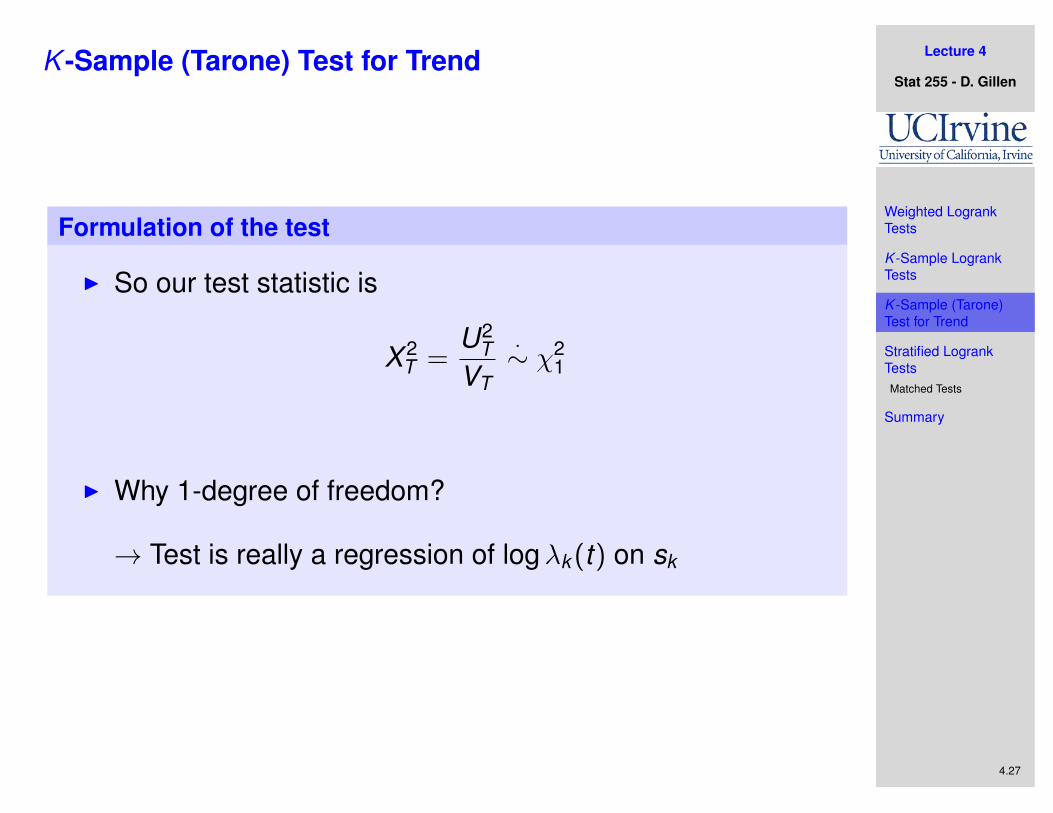
I So our test statistic is

X 2T =

U2T

VT

·∼ χ21

I Why 1-degree of freedom?

→ Test is really a regression of logλk (t) on sk

Lecture 4






Summary

4.28



I There is no dedicated function for the trend test in R, but Ihave written the function survtrend() and posted it onthe course webpage for this purpose

> survtrend( Surv(t2death,death) ~ stage, data=larynx )N Observed Expected

stage=1 33 15 22.5660stage=2 17 7 10.0117stage=3 27 17 14.0845stage=4 13 11 3.3377

Logrank Test : Chi(3) = 22.763, p-value = 4.5252e-05Tarone Test Trend : Chi(1) = 13.815, p-value = 0.00020169

Conclusion: Reject the hypothesis that all four survival curvesare equal and conclude that stage is positively associated withthe hazard for death

Lecture 4






Summary

4.29


Comments

I The trend test depends on the order of the covariate beingtested while the general K -sample test does not

I Why use a trend test (on 1 df) vs. a general K -sample test(on K − 1 df)?

I If effects are monotonically ordered it will be more sensitive

I The general K -sample test has less power because it doesnot take advantage of the ordinal nature of the data

I It seeks to detect a more specific alternative

I If survival curves differ, but differences are not ordered, trendtest less likely to reject

I The trend test is essentially a regression of the hazard onthe covariate of interest

Lecture 4






Summary

4.30

Stratified Logrank Tests

Confounding

I One definition: A confounder is a variable that isassociated with the predictor of interest (X ) and causallyrelated to the outcome of interest (Y ).

Predictor (X ) Outcome (Y )

Confounder (W )

-

HHH

HHHY

��*

HHj

Lecture 4






Summary

4.31


Confounding

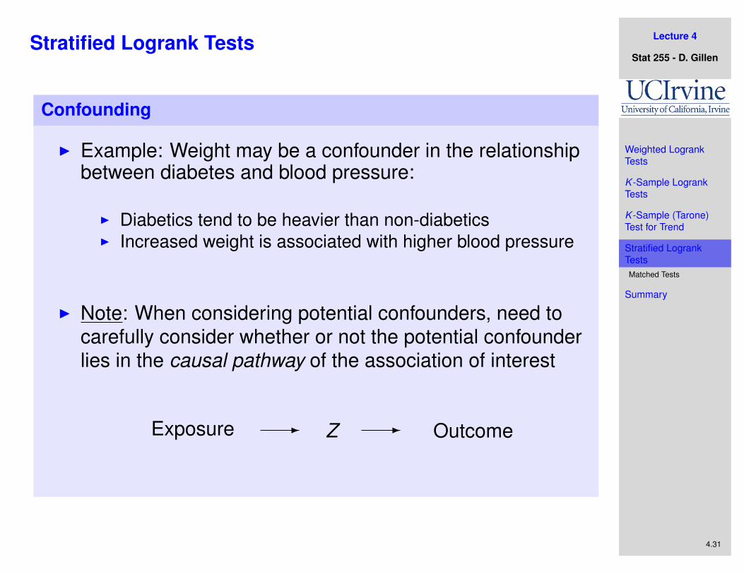
I Example: Weight may be a confounder in the relationshipbetween diabetes and blood pressure:

I Diabetics tend to be heavier than non-diabeticsI Increased weight is associated with higher blood pressure

I Note: When considering potential confounders, need tocarefully consider whether or not the potential confounderlies in the causal pathway of the association of interest

Exposure Z Outcome- -

Lecture 4






Summary

4.32


Confounding

I How do we deal with confounding? Adjust for theconfounder

I Adjustment involves the assumption that the effect ofinterest is similar across all strata of the potentialconfounder

I What if we want to test for differences in risk (ie survivaldata) after adjustment for a potential confounding factor?

→ One solution is to stratify the sample

Lecture 4






Summary

4.33


Set-up and Notation

I Suppose the variable we wish to stratify on has J levels

I Consider testing the hypothesis

H0 : λj1(t) = λj0(t), for j = 1, ..., J and t > 0HA : λj1(t) = φλj0(t), for j = 1, ..., J and t > 0, φ 6= 1

I Notes:

1. λj1(t) can differ from λj′1(t) for two strata j and j ′, as canλj0(t) and λj′0(t)

2. Testing whether, on average across strata j = 1, . . . , J andacross time t , the within-stratum hazard λj1(t) greater (orless) than λj0(t)?

3. Testing for similar (proportional hazards) effects across timeand strata

Lecture 4






Summary

4.34


Set-up and Notation

I Suppose that, for the jth stratumni(j) = the number at risk at time ti(j)

di(j) = the number failing at time ti(j)

I Defineni(j)1 = the number at risk in group 1

and stratum j at time ti(j)

di(j)1 = the number failing in group 1and stratum j at time ti(j)

Lecture 4






Summary

4.35


Set-up and Notation

I Recall: the log-rank test for the j th stratum only wouldcompare “observed” to “expected”:

Uj =∑

i

(obsi(j) − expi(j)) =∑

i

Ui(j)

=∑

i

{di(j)1 − ni(j)1

(di(j)

ni(j)

)}

using the variance

Vj = Var[Uj ] =∑

i

vi(j)

I If Uj is large (positive or negative), then the test will rejectwithin the j th stratum

Lecture 4






Summary

4.36


Set-up and Notation

I The stratified log-rank test sums (averages) over stratajust as the log-rank test sums (averages) over times:

US =∑

j

Uj =∑

j

∑i

Ui(j)

andVS = Var[US] =

∑j

Vj =∑

j

∑i

vi(j)

I Under H0

X 2S =

U2S

VS

·∼ χ21

I The stratified log-rank test statistic US is a weightedaverage of the within-stratum log-rank test statistics Ui

Lecture 4






Summary

4.37


Back to the larynx cancer example...

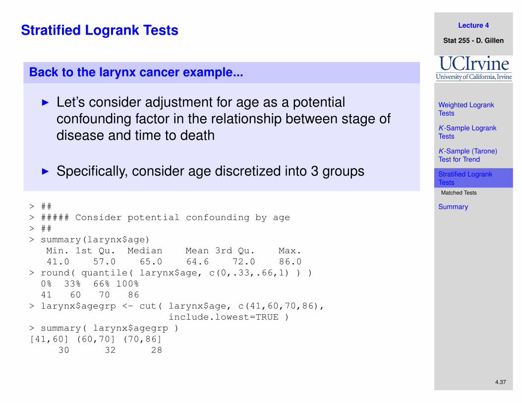
I Let’s consider adjustment for age as a potentialconfounding factor in the relationship between stage ofdisease and time to death

I Specifically, consider age discretized into 3 groups

> ##> ##### Consider potential confounding by age> ##> summary(larynx$age)

Min. 1st Qu. Median Mean 3rd Qu. Max.41.0 57.0 65.0 64.6 72.0 86.0

> round( quantile( larynx$age, c(0,.33,.66,1) ) )0% 33% 66% 100%41 60 70 86

> larynx$agegrp <- cut( larynx$age, c(41,60,70,86),include.lowest=TRUE )

> summary( larynx$agegrp )[41,60] (60,70] (70,86]

30 32 28

Lecture 4






Summary

4.38



I Let’s consider first consider whether or not age is likely tomeet the definition of a confounder...

> ##> ##### Does age meet the definition of a confounder? (not really...)> ##> chisq.test( table( larynx$stage, larynx$agegrp ) )

Pearson’s Chi-squared test

data: table(larynx$stage, larynx$agegrp)X-squared = 4.7134, df = 6, p-value = 0.5811

> survdiff( Surv(t2death,death) ~ agegrp, data=larynx )Call:survdiff(formula = Surv(t2death, death) ~ agegrp, data = larynx)

N Observed Expected (O-E)^2/E (O-E)^2/Vagegrp=[41,60] 30 14 15.9 0.221 0.330agegrp=(60,70] 32 16 20.8 1.103 1.938agegrp=(70,86] 28 20 13.3 3.325 4.615


Lecture 4






Summary

4.39



I From the above, age is not significantly associated withstage or with time to death (in the dataset)

I The implication of this is that adjustment for age is unlikelyto have any impact on the conclusions of our analysis (wewill lose some efficiency though...)

I In a real setting, when testing a well-defined hypothesis weshould decide upon adjustment for age before assessingthe data in order to avoid data-driven inflation of the type 1error rate!

Lecture 4






Summary

4.40



I Let’s stratify by age here as an example...To do this, usethe strata() function in the formula statement ofsurvdiff()

> ##> ##### LR test of association between stage and t2death,> ##### stratified by agegrp> ##> survdiff(Surv(t2death,death) ~ stage + strata(agegrp), data=larynx)Call:survdiff(formula = Surv(t2death, death) ~ stage + strata(agegrp),

data = larynx)

N Observed Expected (O-E)^2/E (O-E)^2/Vstage=1 33 15 23.60 3.134 6.430stage=2 17 7 9.38 0.602 0.763stage=3 27 17 13.23 1.074 1.547stage=4 13 11 3.79 13.686 16.182


Lecture 4






Summary

4.41


Conclusions

I Stage of disease at diagnosis is positively related to therisk of death

I This relationship still holds after adjusting for the effect ofage

I The association is not due to any (positive or negative)association of age with stage of disease and / or age withrisk of death

I The association is not due to any confounding effect ofage

Lecture 4






Summary

4.42

Matched Tests

Matching

I When explicit control for confounders will be difficult,comparative studies are sometime performed on samplesof matched pairs:

I one member of pair is exposed or treated and the other isnot (or gets placebo)

I matching on: age × sex, neighborhood, clinic, etc.

I twins

I matched pairs like many strata of size 2

Lecture 4






Summary

4.43

Matched Tests

Matching

I To account for matching in the sampling scheme, we can:

1. stratify on the matching set,2. compare outcomes within that strata, then3. combine the results across (independent) strata

I As an example, consider the 6-MP data where subjectswere actually matched by remission status and hospital

I One member randomized to 6-MP (vs. placebo)maintenance therapy

Lecture 4






Summary

4.44

Matched Tests

Ex: 6-MP data

I A proper analysis should account for the correlationinduced by matching...

> ##> ##### Matched analysis of the 6-MP data> ##> sixmp <- read.table( "http://www.ics.uci.edu/~dgillen/

STAT255/Data/sixmp.txt" )> sixmp[1:5,]

pairid tpbo t6mp irelapse1 1 1 10 12 2 22 7 13 3 3 32 04 4 12 23 15 5 8 22 1

> ##> ##### Transform data to long format> ##> sixmpLong <- cbind( rep(sixmp$pairid, 2), c(sixmp$tpbo, sixmp$t6mp),+ rep(0:1, each=21), c( rep(1,21), sixmp$irelapse ) )> sixmpLong <- as.data.frame( sixmpLong )> names( sixmpLong ) <- c( "pairid", "time", "sixmp", "irelapse" )

Lecture 4






Summary

4.45

Matched Tests

Ex: 6-MP data

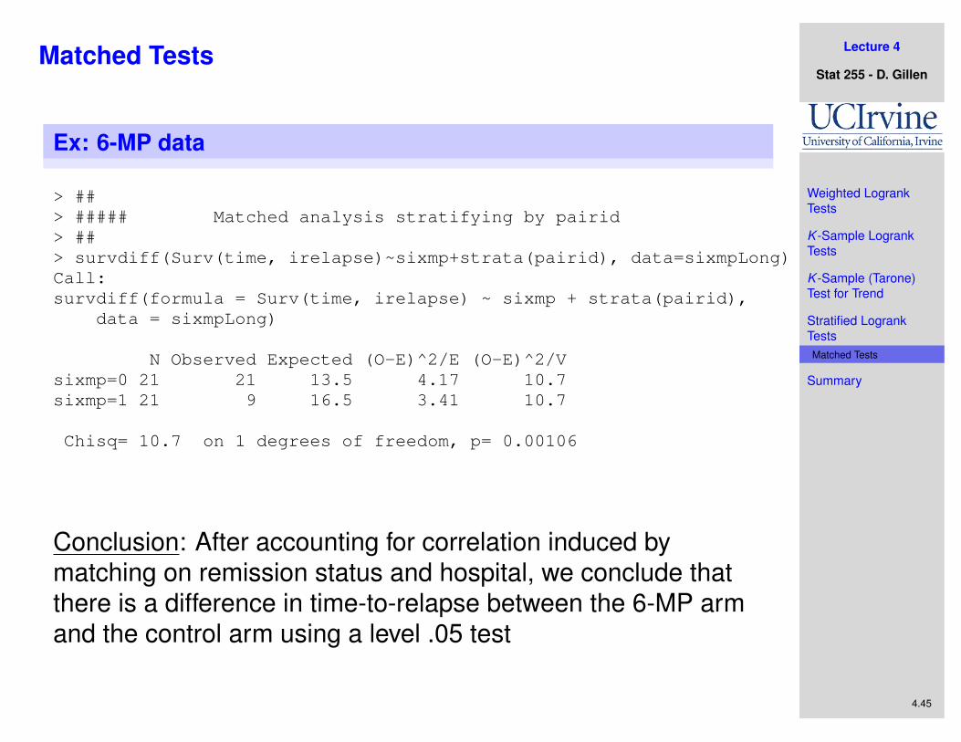
> ##> ##### Matched analysis stratifying by pairid> ##> survdiff(Surv(time, irelapse)~sixmp+strata(pairid), data=sixmpLong)Call:survdiff(formula = Surv(time, irelapse) ~ sixmp + strata(pairid),

data = sixmpLong)

N Observed Expected (O-E)^2/E (O-E)^2/Vsixmp=0 21 21 13.5 4.17 10.7sixmp=1 21 9 16.5 3.41 10.7


Conclusion: After accounting for correlation induced bymatching on remission status and hospital, we conclude thatthere is a difference in time-to-relapse between the 6-MP armand the control arm using a level .05 test

Lecture 4






Summary

4.46

Stratified Analyses

Summary

1. Analyses by separate strata, stratified tests andadjustment are statistical activities, but . . .

I . . . the identification of confounders and the decision toadjust for them are extra-statistical considerations

I . . . they involve (1) the scientific question of interest and (2)possible chains of causality

2. If the study design is stratified or matched, always adjust

3. Stratified tests will have good power for alternatives thatare in the same direction in each stratum

4. When effects are different by stratum (interaction or effectmodification), analyses are better performed and reportedseparately on each stratum

Lecture 4






Summary

4.47

Stratified Analyses

Summary

5. Weighted, K -sample and K -sample trend test versions ofthe stratified log-rank test exist

6. Strata can be quite small for adjustment (but not forwithin-stratum analyses)

7. When data are in the form of matched pairs (or smallsets), think of them as many small strata

8. Stratified log-rank test on matched pairs is the censoreddata analogue of the the signed-rank test for paired data

Lecture 4






Summary

4.48

Stratified Analyses

Analogous Methods For Binomial Data

Proportions Survival Data

1. Description p, RR S, Λ,OR λ, RR

2. Two-sample test Z test/χ2 test Logrank test

3. Stratified two Mantel-Haenzel Stratified-sample test test logrank test

4. K -sample K -sample K -sampleheterogeneity test heterogeneity test logrank test

5. K -sample Cochran-Armitage Tarone trendtrend test trend test test

6. Regression models Logistic regression Cox regression

Documents

Dan Gillen Department of Statistics University of ...dgillen/STAT255/Handouts/lecture4.pdfI Equivalent to the Wilcoxon rank sum statistic when there is no censoring. I The Gˆ; family