Eotvos Lorand University

Faculty of Science

Valentina Halasi

Dantzig-Wolfe Decomposition for CostPartitioning

Applied Mathematician MSc Thesis

Supervisors:

Florian Pommerening

University of Basel, Department of Mathematics and Computer Science

Erika Berczi-Kovacs

Eotvos Lorand University (ELTE), Institute of Mathematics, Department

of Operations Research

Budapest, 2019

Contents

1 Linear Programming 5

1.1 Dantzig-Wolfe Decomposition . . . . . . . . . . . . . . . . . . . . . . . . . 7

2 Classical Planning 11

2.1 Fundamentals . . . . . . . . . . . . . . . . . . . . . . . . . . . . . . . . . . 11

2.1.1 Abstraction Heuristic . . . . . . . . . . . . . . . . . . . . . . . . . . 15

2.1.2 Atomic Projections . . . . . . . . . . . . . . . . . . . . . . . . . . . 16

2.2 Cost partitioning . . . . . . . . . . . . . . . . . . . . . . . . . . . . . . . . 17

2.2.1 Remarks About the Linear Program . . . . . . . . . . . . . . . . . 19

3 Applying the Dantzig-Wolfe Decomposition in Cost Partitioning 20

3.1 Subpolyhedrons . . . . . . . . . . . . . . . . . . . . . . . . . . . . . . . . . 22

3.2 The Master Linear Program . . . . . . . . . . . . . . . . . . . . . . . . . . 23

3.2.1 Reformulation of the Master Linear Program . . . . . . . . . . . . . 25

3.3 An Iteration of the Decomposition Algorithm . . . . . . . . . . . . . . . . 27

3.3.1 Running the Algorithm on the Miconic Example . . . . . . . . . . . 29

4 Computational Experiments 33

4.1 Experimental Setup . . . . . . . . . . . . . . . . . . . . . . . . . . . . . . . 33

4.2 Experiment Results and Analysis . . . . . . . . . . . . . . . . . . . . . . . 34

4.2.1 Heuristic Quality . . . . . . . . . . . . . . . . . . . . . . . . . . . . 35

4.2.2 Running Time and Memory Usage . . . . . . . . . . . . . . . . . . 38

4.2.3 Conclusion and Future Work . . . . . . . . . . . . . . . . . . . . . . 38

2

Introduction

Automated planning is an area of Artificial Intelligence focusing on finding a sequence of

actions for a precisely defined system to reach its goal status. An example for a system

is the Rubik’s cube, and we are looking for a sequence of turnings which leads the initial

state of the cube to the final state. Searching on the large state space is too exhaustive,

but with heuristic search the desired plan can be found effectively. For this we need a

heuristic function as a compass. Cost partitioning combined with abstraction heuristics

results in a strong heuristic function, but computing it requires to solve a large linear

program. Luckily, this linear program has a block structure suitable to apply the Dantzig-

Wolfe decomposition, a classical linear programming tool. In this thesis we apply the

Dantzig-Wolfe decomposition to solve the linear program for cost partitioning in the hope

of finding heuristic functions in a more effective way.

In the first chapter we focus on the fundamentals of linear programming and detail

the general Dantzig-Wolfe decomposition.

The second chapter is an introduction to classical planning, summarizing the necessary

definitions and results leading to the cost partitioning method.

In Chapter 3 we apply the Dantzig-Wolfe decomposition for the cost partitioning linear

program.

We also implemented and tested the method in practice. The description of the ex-

perimental setup and an analysis of the results are summarized in Chapter 4.

3

Acknowledgements

First of all, I would like to thank Florian Pommerening. He has been so generous with his

time, patience, ideas and advices. He is a brilliant mind and the best supervisor a student

could wish for. Thank you for your trust and for all that you teached me.

I would also like to thank Erika Berczi-Kovacs who has supported and motivated me

througout my years at ELTE and she has helped me during this work with her expertise

in operations research.

This master thesis was written during my research internship at the University of

Basel within a framework of the Campus Mundi student mobility program. I would like

to thank the Artificial Intelligence Research Group of the University of Basel and the

Tempus Public Foundation to make this cooperation possible.

I am very thankful to my friends Daniel Racz and Andras Mona, they selflessly helped

me in everything they could during our ELTE years.

Last but not least, I would like to thank Max Gfeller, who helped me not only in

programming and improving this text, but he believed in me and encouraged me the

most.

4

Chapter 1

Linear Programming

This chapter provides the basic definitions and results of linear programming used through-

out this work. Schrijver’s book (1999) is a fundamental literature in the field, and it

contains the proofs for the theorems mentioned.

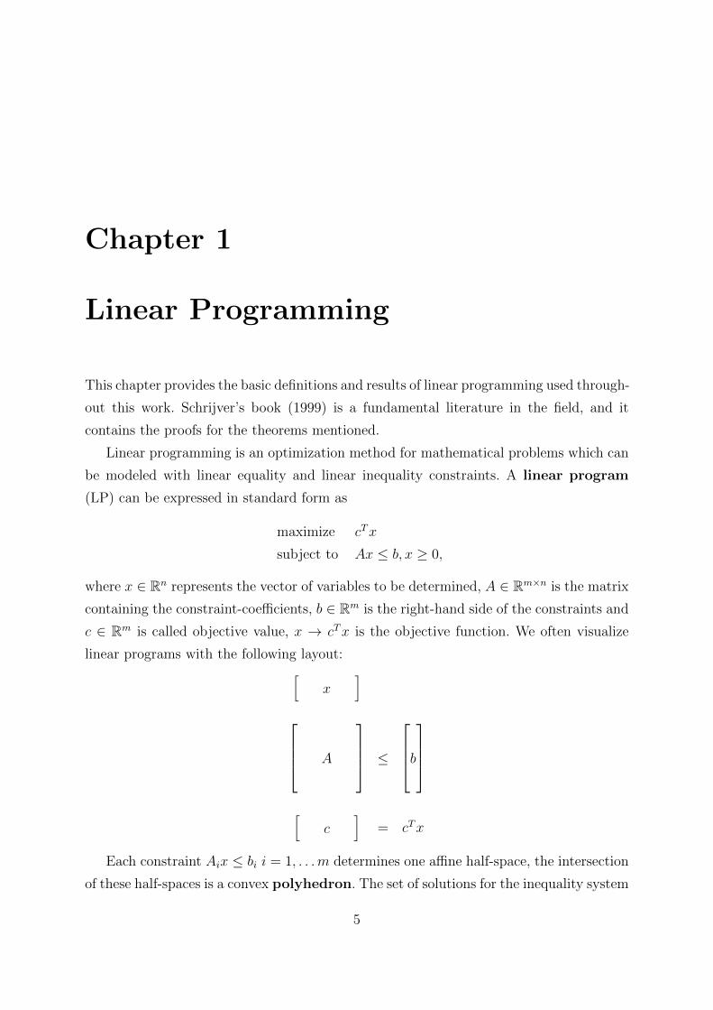
Linear programming is an optimization method for mathematical problems which can

be modeled with linear equality and linear inequality constraints. A linear program

(LP) can be expressed in standard form as

maximize cTx

subject to Ax ≤ b, x ≥ 0,

where x ∈ Rn represents the vector of variables to be determined, A ∈ Rm×n is the matrix

containing the constraint-coefficients, b ∈ Rm is the right-hand side of the constraints and

c ∈ Rm is called objective value, x → cTx is the objective function. We often visualize

linear programs with the following layout:[x

] A

≤

b

[c

]= cTx

Each constraint Aix ≤ bi i = 1, . . .m determines one affine half-space, the intersection

of these half-spaces is a convex polyhedron. The set of solutions for the inequality system

5

{ Ax ≤ b, x ≥ 0 } we call the feasible region. We would like to maximize the linear

function c over this polyhedron. The optimal solution of the LP is x∗ if cTx∗ takes the

maximum value of cTx among all x points in the feasible region. If the feasible region is

nonempty, the problem is feasible, otherwise it is infeasible.

An m-sized set of linear independent column vectors of A {AB1 , AB2 , . . . ABm} we call

a basis B of A. Let us denote by cB and xB the subvectors of c and x belonging to the base

coordinates. The vector z ∈ Rn we call basic solution, if there exists a B nonsingular

submatrix of A, that solving the Bx = b equality results all non-zero coordinates of z.

This means, that z = 0 is also a basic solution of the polyhedron.

This basic solution is unique and it exists, because the matrix B is invertible. A base

B is feasible, if its basic solution x is non-negative in every coordinate. The dual solution

belonging to base B is yB = cBB−1. The reduced cost of base B is δ = yBA− c.

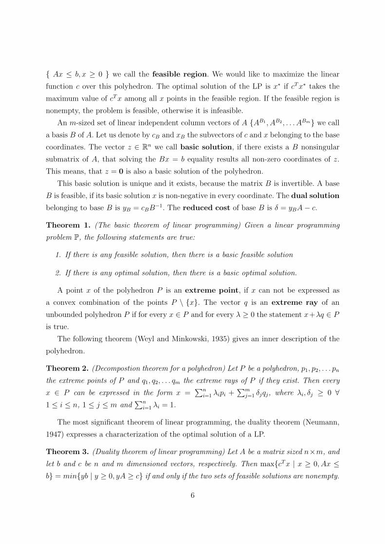
Theorem 1. (The basic theorem of linear programming) Given a linear programming

problem P, the following statements are true:

1. If there is any feasible solution, then there is a basic feasible solution

2. If there is any optimal solution, then there is a basic optimal solution.

A point x of the polyhedron P is an extreme point, if x can not be expressed as

a convex combination of the points P \ {x}. The vector q is an extreme ray of an

unbounded polyhedron P if for every x ∈ P and for every λ ≥ 0 the statement x+λq ∈ Pis true.

The following theorem (Weyl and Minkowski, 1935) gives an inner description of the

polyhedron.

Theorem 2. (Decompostion theorem for a polyhedron) Let P be a polyhedron, p1, p2, . . . pn

the extreme points of P and q1, q2, . . . qm the extreme rays of P if they exist. Then every

x ∈ P can be expressed in the form x =∑n

i=1 λipi +∑m

j=1 δjqj, where λi, δj ≥ 0 ∀1 ≤ i ≤ n, 1 ≤ j ≤ m and

∑ni=1 λi = 1.

The most significant theorem of linear programming, the duality theorem (Neumann,

1947) expresses a characterization of the optimal solution of a LP.

Theorem 3. (Duality theorem of linear programming) Let A be a matrix sized n×m, and

let b and c be n and m dimensioned vectors, respectively. Then max{cTx | x ≥ 0, Ax ≤b} = min{yb | y ≥ 0, yA ≥ c} if and only if the two sets of feasible solutions are nonempty.

6

Consequence 1. In the next chapter of the thesis, we will be using the linear program

max{cTx | Ax = b, x ≥ 0}. The dual pair of this form is min{yb | yA ≥ c} and the duality

theorem holds in this form as well. Let us consider a primal feasible base B of A. The

basic solution xB is optimal if and only if the reduced cost of B yBA− c is non-negative.

This is the constraint we are going to check when looking for an optimal solution of a

linear program.

Linear programming is shown to be solvable in polynomial time (Khachiyan, 1979),

and since then efficient polynomial linear programming methods were developed, which I

summarized in my bachelor thesis (2016). However, the most well-known and used linear

programming algorithm is the Simplex method (Dantzig, 1951), which is the base engine

behind the decomposition method due to Dantzig and Wolfe.

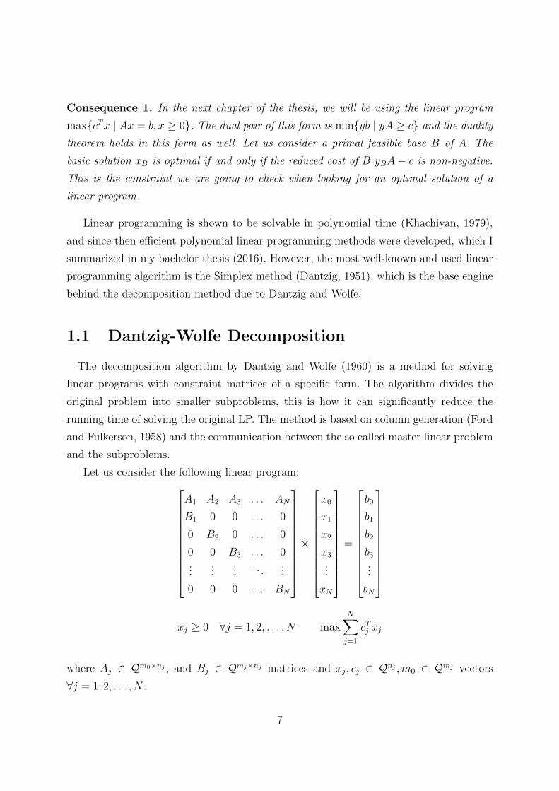
1.1 Dantzig-Wolfe Decomposition

The decomposition algorithm by Dantzig and Wolfe (1960) is a method for solving

linear programs with constraint matrices of a specific form. The algorithm divides the

original problem into smaller subproblems, this is how it can significantly reduce the

running time of solving the original LP. The method is based on column generation (Ford

and Fulkerson, 1958) and the communication between the so called master linear problem

and the subproblems.

Let us consider the following linear program:

A1 A2 A3 . . . AN

B1 0 0 . . . 0

0 B2 0 . . . 0

0 0 B3 . . . 0...

......

. . ....

0 0 0 . . . BN

×

x0

x1

x2

x3...

xN

=

b0

b1

b2

b3...

bN

xj ≥ 0 ∀j = 1, 2, . . . , N max

N∑j=1

cTj xj

where Aj ∈ Qm0×nj , and Bj ∈ Qmj×nj matrices and xj, cj ∈ Qnj ,m0 ∈ Qmj vectors

∀j = 1, 2, . . . , N .

7

If the Aj sub-matrices are zero, the whole problem can be divided to N independent

linear programs. Let us suppose that not all the Aj sub-matrices are zero (the constraints

of the LP A1x1 + A2x2 + . . . ANxN = b0 are called linking constraints) and let us call

the polyhedron defined by the solutions of Bjxj = bj, xj ≥ 0 the polyhedron Pj ∀j =

1, 2, . . . , N . Let us assume that the Pj polyhedron is enclosed by extreme points pjk,

k = 1, 2, . . . lj and extreme rays qjs, s = 1, 2, . . . tj.

According to the decomposition theorem, any point xj of the polyhedron Pj can be

written in the form

xj =

lj∑k=1

λjkpjk +

tj∑s=1

δjsqjs

lj∑k=1

λjk = 1, λjk ≥ 0 ∀k = 1, 2, . . . lj, δjs ≥ 0 ∀s = 1, 2, . . . tj

and any vector in this form will be a solution of the linear program Bjxj = bj, xj ≥ 0.

Using the form above, let us reformulate our original linear program: we will construct

a new linear program which is looking for the λjk and δjs coefficients defined before

involving the linking constraints (∑N

j=1Ajxj = b0) of the original LP:

N∑j=1

( lj∑k=1

(Ajpjk)λjk +

tj∑s=1

(Ajqjs)δjs

)= b0

lj∑k=1

λjk = 1 j = 1, 2, . . . , N

λjk, δj,s ≥ 0 j = 1, 2, . . . , N, k = 1, 2, . . . , lj, s = 1, 2, . . . , tj

maxN∑j=1

cTj

( lj∑k=1

λjkpjk +

tj∑s=1

δjsqjs

)We call this linear program the master problem and it is equivalent to the original

linear program. The master program has m0 + N constraints, while the original linear

program had∑N

i=0mi constraints. The disadvantage of the master linear program is that

it is using many more variables than the original one, since the polyhedron defined by

the solutions of Bjxj = bj can have much more extreme points and rays than the size of

the vector xj. But this factor can be eliminated. We do not have to create the whole LP

with exhaustive calculations to solve it, if we are able to calculate each column one by

one in an iterative way. In linear programs where we do not know all the columns but we

know how to construct them, the column generation method is efficiently usable, since it

8

allows us to ignore a significant part of the linear program during each iteration. The DW

decomposition algorithm generates and uses only a few columns of the master LP at one

iteration. Let us see how this process can be described. The master linear program looks

like this:

[λ11 . . . λ1l1 δ11 . . . δ1s1 . . . δNsN

]

A1p11 . . . A1p1l1 A1q11 . . . A1q1s1 . . . ANqNsN

1 . . . 1 0 . . . 0 0 . . . 0 0

0 . . . 0 0 . . . 0 . . . . . . 0 0...

.... . .

......

0 . . . 0 0 . . . 0 . . . . . . 0 0

=

b0

0...

0

Let us use the following notations: fjk = cTj pjk and gjs = cTj qjs. These are the target

values in the master problem.

Suppose that B is a basis of the matrix of the master problem and let us denote by

xB the basic solution belonging to B, cB the subvector of objective value belonging to the

coordinates of B. Then xB = B−1b and cTBxB is the cost belonging to xB. Now we have

to decide if the basis B is optimal, so we check if it is dual feasible or not.

Let us denote by ωi(i = 1, 2, . . . ,m0) the dual variables belonging to the linking con-

straints and νj(j = 1, 2, . . . , N) the dual variables belonging to the constraints∑lj

k=1 λjk =

1. The dual problem is finding values for the coordinates of the vector (ω, ν) so that

(ω, ν)B = cB. This equality system has a unique solution, (ω, ν) = cBB−1. We proceed

with calculating the reduced cost for checking the dual feasibility.

First the reduced cost belonging to the extreme points:

djk = fTBB−1Ajpjk − fjk = ωTAjpjk + νj − cTj pjk = (ωTAj − cj)pjk + νj

And the reduced cost belonging to the extreme rays:

d′js = fTBB−1Ajqjs − gjs = ωTAjqjs − cTj qjs = (ωTAj − cj)qjs

If the reduced cost is non-negative in every coordinate, the basis is dual feasible, so

it is optimal. If it has a negative coordinate, then we need to perform more iterations.

For this step we have to find the smallest reduced cost, over all extreme points and

extreme rays of all Pj, j = 1, . . . N polyhedrons. Formally, we are looking for the value

9

minj{mink djk,mins d′js} ∀j, k, s , where

minjk

djk = min [ min1≤k≤l1

d1k, min1≤k≤l2

d2k, . . . , min1≤k≤lj

dNk]

minjs

d′js = min [ min1≤s≤t1

d′1s, min1≤s≤t2

d′2s, . . . , min1≤s≤tj

d′Ns]

The formula of the reduced cost shows us that for fixed j, the point of the polyhedron

Pj taking the value min{mink djk,mins d′js} is always an extreme point or extreme ray of

the polyhedron defined by the feasible solutions of Bjxj = bj. Since every extreme point

and ray of the system Bjxj = bj is a feasible basic solution, mink,s{min djk,min d′js} will

be the sum of νj and the solution of the following LP problem:

Bjxj = bj xj ≥ 0 min(ωTAj − cj)xj

An optimal basic solution of this LP will provide us an extreme point pjk or ex-

treme ray qjs, and the djk or d′js belonging to the given j index will be minimal for

every 1 ≤ k ≤ lj or 1 ≤ s ≤ tj. We have to calculate an optimum N times with

solving N small LP problems, let us denote by O∗j the optimum of jth problem. Then

minj{mink djk,mins d′js} = minj (O∗j + νj) will give us the smallest reduced cost. If this is

non-negative, then our solution is optimal, due to the minimality the other coordinates

of the reduced cost will be non-negative as well. If this is negative, we involve the column

belonging to this coordinate in the LP in the basis. The basis column which we will erase

of our basis can be chosen according to the rules used in the simplex method: if we choose

the column with the smallest index, the algorithm will terminate. We repeat these steps

until we find a primal and dual feasible basic solution. According to the finiteness of the

simplex method, the DW algorithm terminates after a finite number of iterations.

10

Chapter 2

Classical Planning

2.1 Fundamentals

In this chapter we focus on the theory of AI Planning, a branch of Artificial Intelligence.

Planning is creating a sequence of predefined actions, to transform the initial state of the

world to one of the given goal states. The aim is either finding a satisfying plan or the

cheapest plan for given operator costs. The problems can be considered as path-finding

tasks in the graph of the state space. The state space is exponential in the size of the

input, so the classical dynamic programming shortest path finding algorithms like the

Dijkstra algorithm (1959) are not efficiently applicable.

A simple miconic planning optimization task is the following: an elevator can operate

between the ground floor f0 and the first floor f1, it is initially on f0. A passenger is

initially on f1, she would like to reach f0 with the elevator. All actions (the elevator goes

up, the elevator goes down, the passenger boards, the passenger departs) have cost 1.

What is the cheapest plan to reach the goal state (the passenger is departed on f0)?

In most planning problems, the conditions are not this easy to describe and we need

a uniform language to define a planning task of any complexity. The following definition

(Backstrom and Nebel, 1993) is a formal description of planning tasks:

Definition 1. A SAS+ planning task is a 4-tuple: Π =⟨V,O, s0, S

∗⟩, where

1. V is a finite set of state variables, each variable v ∈ V with a finite domain dom(v).

The situation in the world can be described with assigning to the state variables

one of the values in their domain. The assignment can be determined for all state

variables (we call this a variable assignment), or to the subset of the state variables

11

(partial variable assignment). Let V be a set of state variables. A function f : V →⋃v∈V

dom(v) is a variable assignment over V if f(v) ∈ dom(v) for all variables v ∈ V.

We write the domain of a (possibly partial) variable assignment f as vars(f).

A variable assignment over V is a state. The set of all states over V is S. For a

partial variable assignment s1 and a state s2 we say, that s1 ⊆ s2, if s1(v) = s2(v)

for all v ∈ vars(s1).

2. O is a finite set of operators, where each o ∈ O has the following components:

• preconditions: pre(o) (partial variable assignment)

An operator o can be executed in state s, if s meets o’s preconditions: pre(o) ⊆ s.

• effects: eff(o) (partial variable assignment)

If o is applicable in s, the effect of o determines the resulting state s′:

s′ = s[o] with s[o](v) = eff(o)(v) for all v ∈ vars(eff(o)), s[o](v) = s(v) for all

other variables

• the cost function cost(o), where cost : O → R≥0

3. s0 is the initial state (variable assignment)

4. S∗ is the goal description (partial variable assignment)

Pommerening and Helmert (2015) have shown, that planning tasks can be efficiently

converted to transition normal form:

Definition 2. A planning task Π is in transition normal form, if vars(pre(o)) = vars(eff(o))

for all operators o ∈ O and S∗ is one state.

The convertion can be done using the following steps:

• A new value u is added to the domain of every variable in v ∈ V .

• For every variable v and for every value w ∈ dom(v) we add a forget operator with

precondition v 7→ w, effect v 7→ u and cost 0.

• For all variables v and operators o, if the value of v is determined in pre(o) but not

in eff(o), then we add v 7→ pre(o)[v] to eff(o). If the value of v is determined in

eff(o) only, then we add v 7→ u to pre(o).

12

• If the value of a variable v is not determined in the goal state, then we add v 7→ u

to the goal description.

In the experiments detailed in Chapter 4, the example planning tasks were converted

to this restricted structure.

The definition of the miconic planning task in the SAS+ formalism is the following:

Π =⟨V,O, s0, S

∗⟩, where

1. V = {v0, v1, v2} and dom(v0) = dom(v1) = dom(v2) = {0, 1}.v0 is the variable describing the position of the elevator. Variable v1 defines if the

passenger p0 is boarded (v1 = 0) or not boarded (v1 = 1). Variable v2 shows if the

passenger p0 is departed (v2 = 0) or not departed (v2 = 1).

2. O = {

• boardf1p0 , preconditions: v0 = 1, v1 = 1, effect: v1 = 0, cost(boardf1p0) = 1

• departf0p0 , preconditions: v0 = 0, v1 = 0, v2 = 1, effects: v1 = 1, v2 = 0,

cost(departf0p0) = 1

• downf1f0, precondition: v0 = 1, effect: v0 = 0, cost(downf1f0) = 1

• upf0f1, precondition: v0 = 0, effect: v0 = 1, cost(upf0f1) = 1

}

3. s0 = (0, 1, 1)

4. S∗ : v2 = 0

The transition system of a planning task describes the state space of the problem,

which helps us to visualize the task as path-finding in a graph:

Definition 3. A transition system is a tuple⟨S, L, T, s0, S

∗G, cost

⟩:

• S: finite set of states

• L: finite set of transition labels

• T : a set of labeled transitions⟨s, l, s′

⟩with s, s′ ∈ S, l ∈ L

• si ∈ S the initial state

13

• SG ⊆ S the goal states

• cost : L→ R≥0 cost function

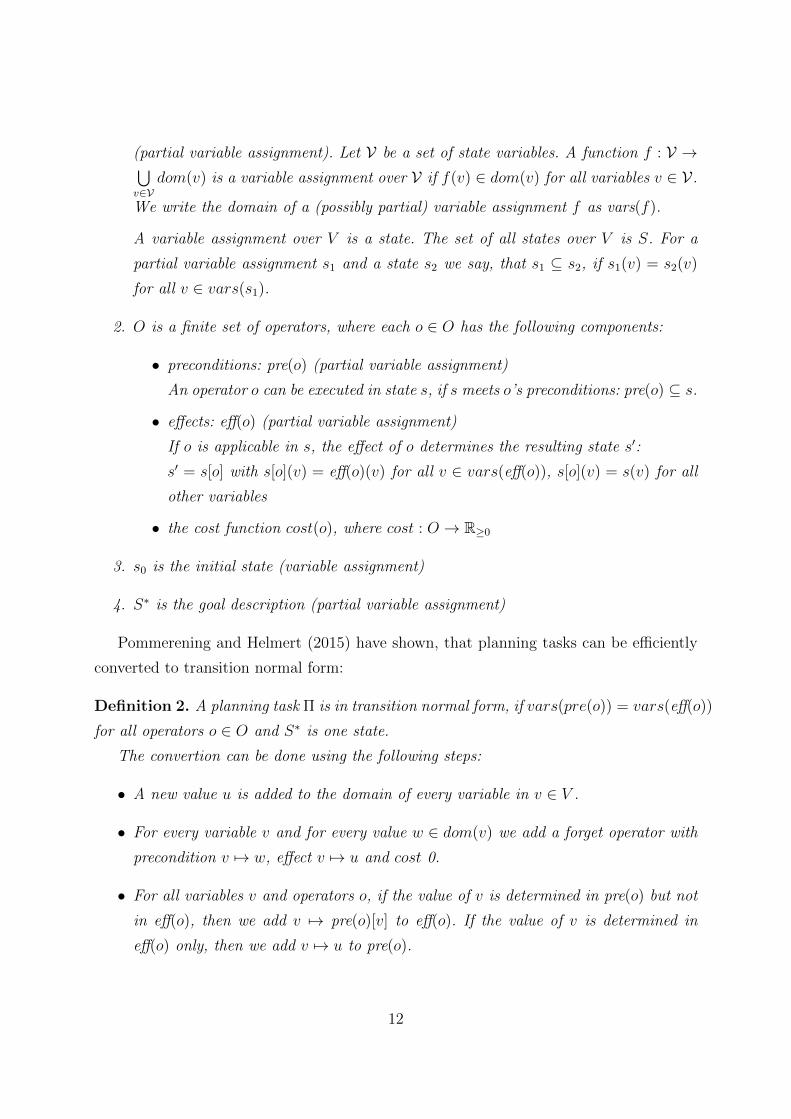
Figure 2.1 visualises the transition system of the miconic task. One arrow on the graph

denotes one transition, the initial state is marked with the bold arrow and goal states are

marked with green frame.

1,1,0 1,1,1

0,1,0 0,1,1 0,0,0

1,0,0 1,0,1

0,0,1

elevatoron f1

elevatoron f0

board board

depart

depart

up up up updown down down down

Figure 2.1: The state space of the miconic planning task.

A SAS+ task Π induces a transition system: the states are the states of Π, the tran-

sition labels are the operators, a transition⟨s, o, s′

⟩is in T iff pre(o) ⊆ s, s′ = s[o]. Each

state in the set of goal states of the transition system meets the assignments defined in

the partial variable assignment of the goal description in Π, and the goal states are the

states satisficing the goal description. Last, the initial state is the same in both concepts.

Definition 4. A plan for a SAS+ planning task Π is a path from the initial state to one

of the goal states in the transition system induced by Π.

The planning problem is the following: the input is a planning task for example in

SAS+ formalism, and we have to find a plan which is feasible or to show that an appro-

priate plan does not exist. This we call satisficing planning, but in this thesis we are only

interested in optimal planning.

Definition 5. A plan which uses operators with the minimum sum of operator costs

among all plans is called an optimal plan. In optimal planning, the goal is to find an

14

optimal plan. In other words, we would like to find a cheapest path from the start state to

a goal state in the transition system of the planning task.

A way of finding a solution for an optimal planning problem is with heuristic search

(Pearl, 1984). A well-known method is the A∗ algorithm (Hart et al., 1968) combined with

an admissible heuristic.

Definition 6. A heuristic is a function on the states h : S → R≥0 ∪ {∞}. For all s ∈ S,

h(s) gives an estimation for the cost of getting to a goal state from the state s .

Definition 7. The optimal heuristic, h∗ is the function which gives us the cheapest cost

of getting from a given state to a goal state for the given cost function (or∞ if no optimal

plan exist).

Definition 8. An admissible heuristic h is a heuristic which never estimates over the

optimal cost: h(s) ≤ h∗(s) ∀s ∈ S.

Definition 9. Suppose that for two heuristics h1, h2 the inequality h1(s) ≤ h2(s) holds

for all states s ∈ S. Then we say, that the heuristic h2 dominates h1.

The next section explains how to derive an admissible heuristic.

2.1.1 Abstraction Heuristic

We consider the so-called abstraction heuristics. With an abstraction we “narrow” the

state space, and we get a relaxed planning task, which is easier to solve than the original

planning problem. All transitions are represented in the abstraction, so every plan for the

original task is still a plan in the abstract system.

Definition 10. Let Π be a planning task and 〈S, L, T, s0, S∗⟩

its transition system. An

abstraction mapping ϕ is a function ϕ : S → Sϕ that maps states to abstract states. The

resulting induced abstraction has the transition system 〈Sϕ, L, Tϕ, sϕ0 , Sϕ∗⟩, where

• for every transition 〈s, o, s′〉 ∈ T there is a transition in the abstract system 〈ϕ(s), o, ϕ(s′)〉 ∈Tϕ and there are no other transitions in Tϕ

• sϕ0 = ϕ(s0)

• ϕ(s∗) ∈ S∗ϕ for all s∗ ∈ S∗ and there are no other states in S∗ϕ

15

Consequence 2. If p : 〈o1, o2, . . . on〉 is a path in the original system between s1, s2 ∈ S,

the same path is a path in S ′ from ϕ(s1) to ϕ(s2) with cost(p) = cost(p′).

Definition 11. The heuristic derived by the abstraction for state s is the shortest path

from ϕ(s) to any abstract goal state.

hϕ(s) = h∗Sϕ(ϕ(s))

Remark 1. According to Consequence 2, the least cost path from s to a goal state in the

original transition system exists with the same cost in the abstract system and leads to an

abstract goal state. The least cost path from ϕ(s) to an abstract goal state in the abstract

transition system can not have greater cost. This is why hϕ is an admissible heuristic.

2.1.2 Atomic Projections

We define an abstraction type which will be used in the computational experiments, this

is the atomic abstraction. For a fixed variable v ∈ V we consider the effect of the operators

on v only. We first define the state space of this abstraction:

Definition 12. The state space of the atomic projection to v is a directed graph on

nodes dom(v). It has an edge from w ∈ dom(v) to w′ ∈ dom(v) labeled by operator o if

pre(o)[v] = w and eff(o)[v] = w′ or if v /∈ vars(pre(o)) and eff(o)[v] = w′. If there is an

operator with v /∈ pre(o) and v /∈ eff(o) then it has a self-loop on all abstract states.

The abstract initial state of the abstraction is the variable from dom(v) which is

assigned to v in s0. The abstract goal state is the variable from dom(v) which is assigned

to v in S∗, this is clearly determined if the task is in transition normal form.

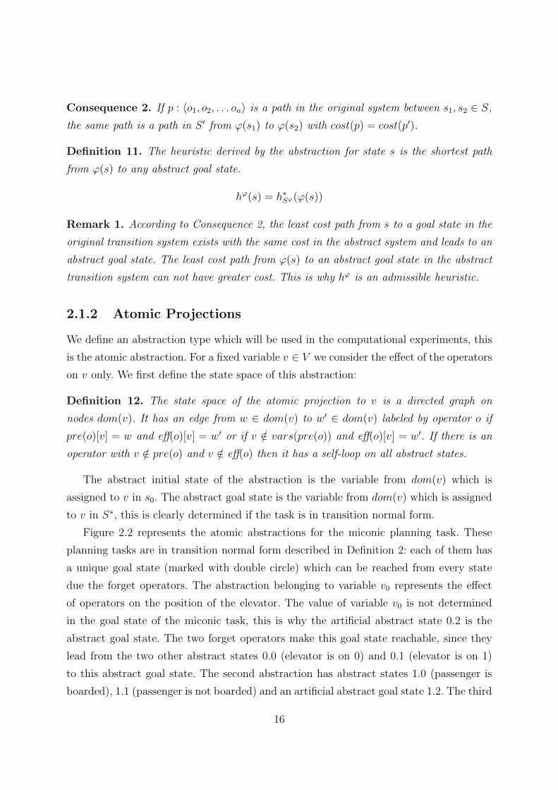
Figure 2.2 represents the atomic abstractions for the miconic planning task. These

planning tasks are in transition normal form described in Definition 2: each of them has

a unique goal state (marked with double circle) which can be reached from every state

due the forget operators. The abstraction belonging to variable v0 represents the effect

of operators on the position of the elevator. The value of variable v0 is not determined

in the goal state of the miconic task, this is why the artificial abstract state 0.2 is the

abstract goal state. The two forget operators make this goal state reachable, since they

lead from the two other abstract states 0.0 (elevator is on 0) and 0.1 (elevator is on 1)

to this abstract goal state. The second abstraction has abstract states 1.0 (passenger is

boarded), 1.1 (passenger is not boarded) and an artificial abstract goal state 1.2. The third

16

abstraction has the abstract goal state 2.0 (the passenger is departed), abstract state 2.2

(the passenger is not departed) and an artificial abstract state 2.2.

0.2 1.2 2.21.10.1

0.0 1.0 2.0

2.1

board

board

depart

depart departup

downforget_var0_val0

forget_var0_val1

forget_var1_val0

forget_var1_val1

forget_var2_val0

forget_var2_val1

Figure 2.2: Atomic abstractions for variables v0, v1 and v2 of the miconic example. The

heuristic values of these three abstractions are 0, 0 and 1. Taking their maximum gives

an admissible heuristic for the planning task, 1. With cost partitioning we can combine

them to reach a higher heuristic value.

2.2 Cost partitioning

When we have a set of n admissible heuristics for a task (for example we consider n

abstractions and their corresponding heuristics), we can take the maximum of their cost

and the corresponding heuristic is an admissible heuristic dominating each individual

heuristic from the set. But it would be better to use the information given by the other

n− 1 heuristics in the hope of getting a cost-estimation closer to the optimum. The sum

of admissible heuristics is not admissible. Cost partitioning (Katz and Domshlak 2007 ,

Katz and Domshlak 2008, Yang et al. 2008, Katz and Domshlak 2010) is a method for

additively combining different heuristic estimates while guaranteeing admissibility of the

combination. Let Π =⟨V,O, s0, S

∗, cost⟩

be a planning task and let costi : O → R+0 for

1 ≤ i ≤ n be a family of cost functions such that∑n

i=1 costi(o) ≤ cost(o) ∀o ∈ O (this

we call the cost partitioning condition). If {h1, h2, . . . hn} is a set of admissible heuristics

so that hi is an admissible heuristic for Πi =⟨V,O, s0, s

∗, costi⟩, then

∑ni=1 hi is also an

admissible heuristic for Π. So a set of cost functions {costi}ni=1 can be a valid partition

of operator costs if the cost partitioning condition is satisfied. Different cost partitionings

lead to additive heuristics of different quality, the question is how to derive a good cost

partitioning.

17

Let us denote by A the set of abstractions we are using, let α ∈ A be an abstraction.

In the transition system formalism let us denote by T α the abstract transition system,

Sα the abstract states, Tα the abstract transitions, S∗α the set of goal states belonging

to the abstraction α.

Definition 13. We call a state s ∈ S dead state, if a plan can reach it, but it is impossible

to reach a goal state from s, or if no plan can reach it.

Since they would just slow down the computations without contribution to the objec-

tive function, let us remove all the dead states from the transition systems T α ∀α ∈ A.

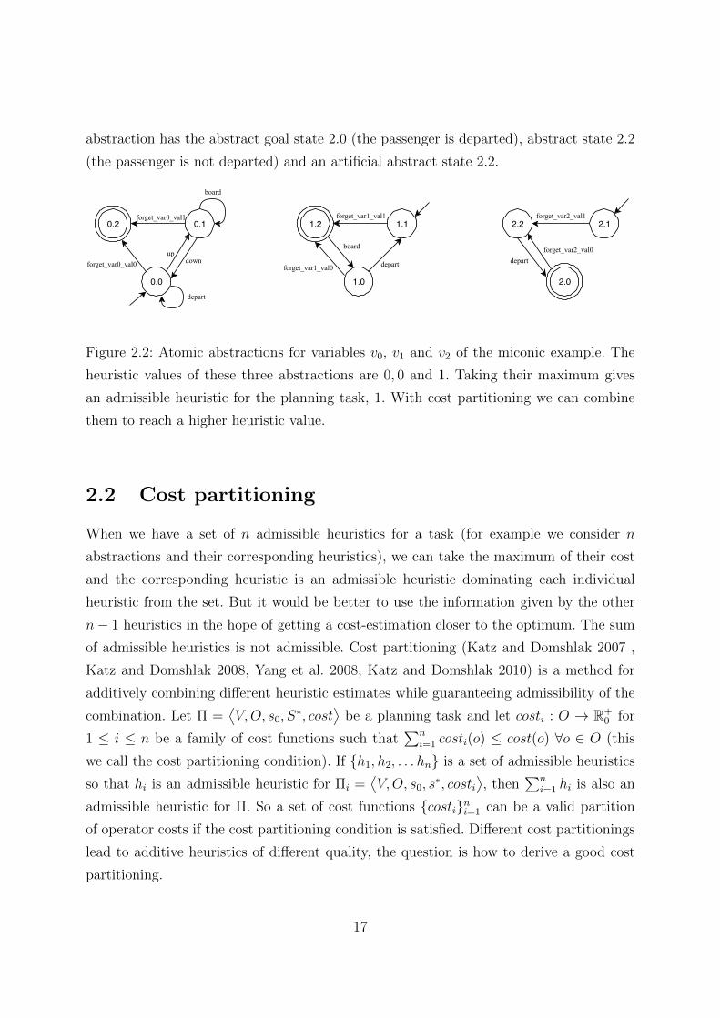
After describing the notations, the following linear program will give us an estimation

for optimal cost partitioning belonging to the abstractions in A. We get this estimation

iff the polyhedron defined in the LP is bounded in the direction of the objective function.

If this is not the case, the result is ∞. The linear program for cost partitioning was

introduced by Katz and Domshlak (2008) and can be modelled in slightly different ways.

We use the notation of Roger and Pommerening (2015).

Linear program for optimal cost partitioning:

• Variable Cαo ∀α ∈ A, ∀o ∈ O which occurs in the transitions Tα.

This variable assigns a cost to the operator o in the transition system T α.

• Variable Dαs′ ∀α ∈ A, for all s′ ∈ Sα abstract state of abstraction α

This variable gives us the exact cost of the cheapest path from the abstract state of

the initial state to s′ in T α according to the cost function determined by Cαo .

• Variable Hα ∀α ∈ AThe heuristic estimation for abstraction α - the lowest cost for getting from the

initial state to any goal state in the abstract system belonging to α.

maximize∑α∈A

Hα

subject to Dαs′ = 0 ∀α ∈ A, s′ = α(s0)

Dαs′′ ≤ Dα

s′ + Cαo ∀α ∈ A,∀

⟨s′, o, s′′

⟩∈ Tα

Hα ≤ Dαs′ ∀α ∈ A,∀s′ ∈ S∗α∑

α∈A

Cαo ≤ cost(o) ∀o ∈ O

0 ≤ Dαs′ , H

α ∀o ∈ O,α ∈ A, s′ ∈ Sα

18

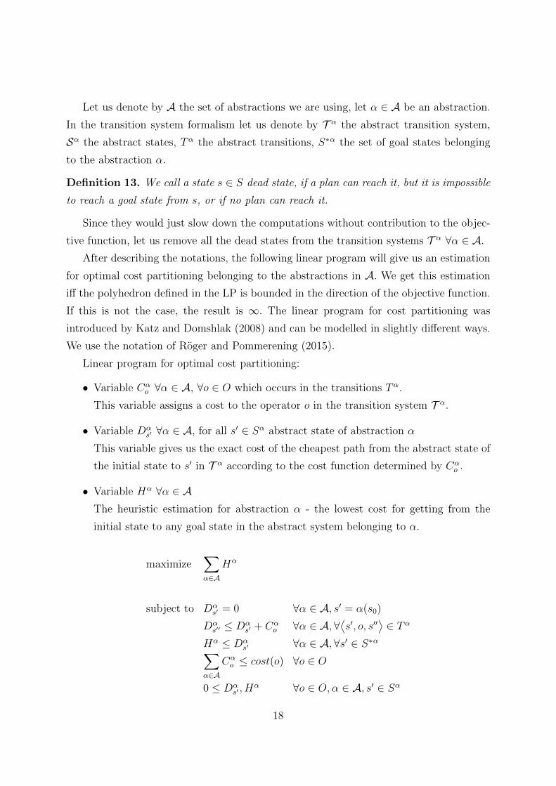
The first constraint shows, that for each abstraction in its own abstract transition

system it is costless to get from the abstract initial state to the same abstract state. The

second constraint expresses a triangle inequality - it has to be satisfied because Dαs′ denotes

a cost of a cheapest path. The third constraint requires the minimality of the heuristic

function among all plans starting from the initial state, ending in the goal state. The

fourth is the cost partitioning constraint, it brings in the definition of cost partitioning

to the LP. The last constraints insure that the path-length variables are non-negative.

For the cost variables it is not necessary, due to general cost partitioning (Pommerening

et al., 2015) to the variable Cαo we can assign negative values too.

2.2.1 Remarks About the Linear Program

Some remarks are worth mentioning about the linear program for cost partitioning, since

it is not obvious, why is this a correct linear program and where the formalization of the

”cheapest path” is hiding.

Shortest path - feasible potential

Let D = (V,A) a directed graph, let us denote by Q the incidence matrix of D. We

say that the vector π : V → R is a feasible potential for the cost function c : A → R, if

π(v)−π(u) ≤ c(uv) is true for every edge uv ∈ A. In other words, the potential is feasible

if and only if πQ ≤ c.

Using the duality theorem by Neumann, the connection between the potential and the

shortest path problem is visible:

Theorem 4. If c is conservative, the cost of the cheapest path from s to t in D is equal

to max{π(t)− π(s)}, where the maximum is considered on all feasible potentials.

The theorem says that finding the maximum of the potential problem (dual problem)

is equivalent to the shortest path problem (primal problem). In the cost partitioning LP

the transitions with operator costs are the edges with cost function and the abstract states

are the vertices of the directed graph which represents the abstract transition system. Let

us notice that the constraints Dαs′′ ≤ Dα

s′+Cαo ∀α ∈ A, ∀

⟨s′, o, s′′

⟩∈ Tα are equivalent

with the constraints of the feasible potential problem. The constraint Dαs′ = 0 ∀α ∈

A, s′ = α(s0) will make the variables represent the cost of the shortest path from the

initial abstract state. This is why we do not have to formulate the shortest path problem

in the LP, since solving the dual of the shortest path problem is sufficient and simpler.

19

Chapter 3

Applying the Dantzig-Wolfe

Decomposition in Cost Partitioning

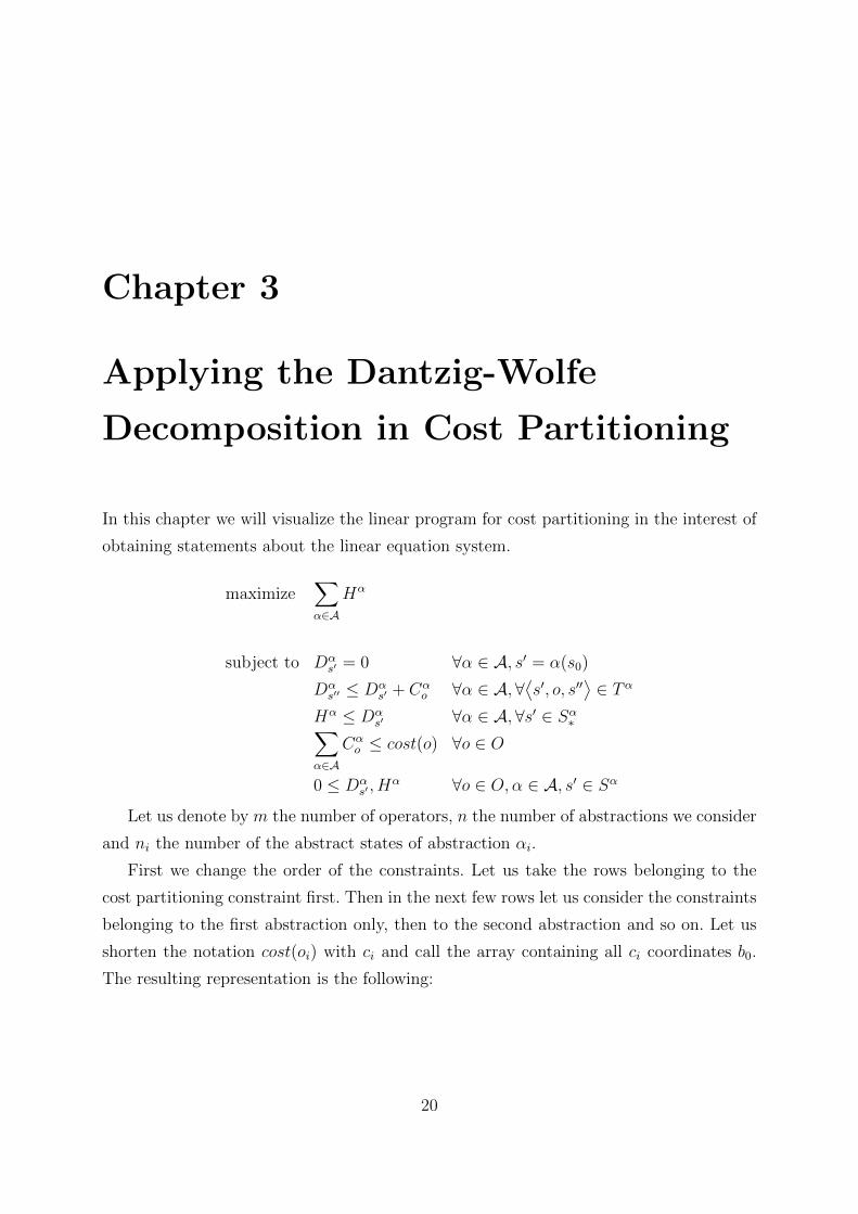
In this chapter we will visualize the linear program for cost partitioning in the interest of

obtaining statements about the linear equation system.

maximize∑α∈A

Hα

subject to Dαs′ = 0 ∀α ∈ A, s′ = α(s0)

Dαs′′ ≤ Dα

s′ + Cαo ∀α ∈ A,∀

⟨s′, o, s′′

⟩∈ Tα

Hα ≤ Dαs′ ∀α ∈ A,∀s′ ∈ Sα∗∑

α∈A

Cαo ≤ cost(o) ∀o ∈ O

0 ≤ Dαs′ , H

α ∀o ∈ O,α ∈ A, s′ ∈ Sα

Let us denote by m the number of operators, n the number of abstractions we consider

and ni the number of the abstract states of abstraction αi.

First we change the order of the constraints. Let us take the rows belonging to the

cost partitioning constraint first. Then in the next few rows let us consider the constraints

belonging to the first abstraction only, then to the second abstraction and so on. Let us

shorten the notation cost(oi) with ci and call the array containing all ci coordinates b0.

The resulting representation is the following:

20

[ xα1︷ ︸︸ ︷[Dα1s0. . . Dα1

sn1Hα1Cα1

o1. . . Cα1

om

] xα2︷ ︸︸ ︷[Dα2s0

. . .]

. . .

xαn︷ ︸︸ ︷[Dαns0

. . .] ]}x

M1︷ ︸︸ ︷ 01 . . . 0...

. . ....

0 . . . 1

M2︷ ︸︸ ︷0

1 . . . 0...

. . ....

0 . . . 1

. . .

Mn︷ ︸︸ ︷01 . . . 0...

. . ....

0 . . . 1

α1

0 0 0

0

α2

0...

... 0 . . . 0

0 . . . 0

αn

︸ ︷︷ ︸

A

≤

≤

c1...

cm

0...

...

0

︸ ︷︷ ︸

b[ [0 . . . 0 1 0 . . . 0

][0 . . .

]. . .

[0 . . .

] ]}c

The sub-matrix of the cost partitioning constraints expresses the dependence between

the abstractions. This sub-matrix consists of n matrices M1,M2, . . .Mn next to each

other. The Mj matrix belongs to the j’th abstraction, Mj consists of a zero-matrix sized

m × (nj + 2) and an identity matrix sized m × m next to it. The remaining part of

the LP-matrix consists of diagonal blocks, one for each of the n abstractions. All the

constraints belonging to an abstraction αi ∈ A have a row vector independent from a row

vector belonging to a constraint of an other abstraction αj ∈ A in the matrix. This is

why block matrices occur: each abstraction αi ∈ A has its own non-zero matrix-block αi

(visualized later), otherwise the column-coordinates of the whole LP matrix belonging to

the abstraction are zero. This is exactly the form that the Danzig-Wolfe decomposition

method requires.

For the sake of accuracy two little changes have to be performed in the form the

linear program: most of the constraints have less-than-or-equal relations, although the

decomposition was defined with equality. With non-negative slack variables attached to

each non-cost-partitioning constraint this can be solved.

21

Furthermore, the solution in the Dantzig-Wolfe decomposition has to be non-negative,

which is also required by the slack-variables and by the variables Dαs′ , H

α ∀α ∈ A, s′ ∈ Sα,

but not by the variables Cαo . The solution for this is two variables for each Cα

o : one,

Cα+o remains the same and also the matrix-colum which belongs to it, the other, Cα−

o is

responsible for the negative values Cαo can have, the same matrix-column multiplied by

(−1) belonging to it.

LP solvers like CPLEX can easily handle these limitations without us having to add slack

variables and plus-minus variables.

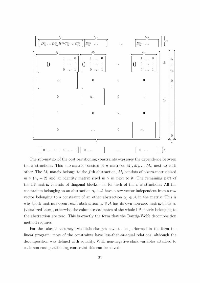
3.1 Subpolyhedrons

In the linear program for cost-partitioning the linking constraints of the Danzig-Wolfe

decomposition are the cost-partitioning constraints. The Pj polyhedron defined in the

decomposition belongs to the j’th abstraction: the points of them are the solutions of the

linear equation system αjxαj = 0, xαj ≥ 0.

Namely xαj = (Dαjs0 . . . D

αjsnjHαjC

αj00. . . C

αjom) is in the polyhedron Pj

if Dαjs′ = 0 where s′ = αj(s0)

Dαjs′′ ≤ Dαi

s′ + Cαio ∀

⟨s′, o, s′′

⟩∈ Tαi

Hαi ≤ Dαis′ ∀s′ ∈ Sαi∗

0 ≤ Dαis′ , H

αi ∀o ∈ O, s′ ∈ Sαi

and the visualization looks as follows:

[Dαjs1 D

αjs1 . . .

goal states︷ ︸︸ ︷Dαjsn1−1 D

αjsn1

Hαj Cαjo1 C

αjo2 . . . C

αjom−1 C

αjom

]

Qαj

0

0

0

0

0 . . . −1 . . .

−1 0 . . .

0 0 . . . −1

. . .

−1 0 0

0 0. . . 0

0 . . . −1

1

1

1

0 . . .

0 . . .

0 . . .0

≤

0

...

0

The (Qαj) is the incidence matrix of the directed graph belonging to Tα. One row

denotes one directed edge (operation), and in the same row we write −1 to the corre-

22

sponding operator variable in the upper-right block. The bottom-left block matrix is all

zero, except of the columns of the goal states variables with −1 entries. These rows express

the constraints Hα ≤ Dαs′ ∀α ∈ A,∀s′ ∈ Sα∗ .

If we evoke the feasible potential view for this linear program we can note the following:

due to the linear constraints and the restriction Dαs′ = 0 ∀α ∈ A, s′ = α(s0), an extreme

point of the polyhedron Pj will give us a feasible potential, and this potential determines

the cost of the shortest paths in the directed graph belonging to the transition system

T αj . These shortest paths depend on the cost function [Cαjo1 , C

αjo2 . . . C

αjom−1, C

αjom ], which is

part of the feasible potential.

When applying the Dantzig-Wolfe decomposition, in every iteration the master linear

program (detailed in the next section) will ask for an extreme point or extreme ray of

these Pj polyhedrons, depending on a changing cost function.

3.2 The Master Linear Program

In this section, we will discuss the master linear program of the Dantzig-Wolfe decompo-

sition for the linear program for cost-partitioning.

Let us denote by pjk, k = 1, 2, . . . lj and qjs, s = 1, 2, . . . tj the extreme points and

extreme rays which bound the polyhedron Pj. Every point xαj in Pj can be written in the

form

xαj =

lj∑k=1

λjkpjk +

tj∑s=1

δjsqjs

lj∑k=1

λjk = 1, λjk ≥ 0 ∀k = 1, 2, . . . lj δjs ≥ 0 ∀s = 1, 2, . . . tj

and any vector in this form will be a solution of the linear program αjxαj = 0, xαj ≥ 0.

Using the new form of the polyhedron-point xαj , we get the following linear program,

which is the master linear program of the linear program for cost partitioning:

n∑j=1

( lj∑k=1

(Mjpjk)λjk +

tj∑s=1

(Mjqjs)δjs

)= b0 (3.1)

lj∑k=1

λjk = 1 j = 1, 2, . . . , n

λjk ≥ 0, δjs ≥ 0 j = 1, 2, . . . , n, k = 1, 2, . . . , lj s = 1, 2, . . . , tj

23

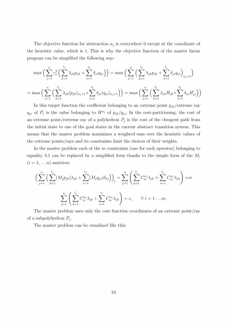
The objective function for abstraction αj is everywhere 0 except at the coordinate of

the heuristic value, which is 1. This is why the objective function of the master linear

program can be simplified the following way:

max( n∑j=1

cTj

( lj∑k=1

λjkpjk +

tj∑s=1

δjsqjs

))= max

( n∑j=1

( lj∑k=1

λjkpjk +

tj∑s=1

δjsqjs

)nj+1

)

= max( n∑j=1

( lj∑k=1

λjk(pjk)nj+1+

tj∑s=1

δjs(qjs)nj+1

))= max

( n∑j=1

( lj∑k=1

λjkHjk+

tj∑s=1

δjsH′js

))In this target function the coefficient belonging to an extreme point pjk/extreme ray

qjs of Pj is the value belonging to Hαj of pjk/qjs. In the cost-partitioning, the cost of

an extreme point/extreme ray of a polyhedron Pj is the cost of the cheapest path from

the initial state to one of the goal states in the current abstract transition system. This

means that the master problem maximizes a weighted sum over the heuristic values of

the extreme points/rays and its constraints limit the choices of their weights.

In the master problem each of the m constraints (one for each operator) belonging to

equality 3.1 can be replaced by a simplified form thanks to the simple form of the Mi

(i = 1, . . . n) matrices:

( n∑j=1

( lj∑k=1

(Mjpjk)λjk +

tj∑s=1

(Mjqjs)δjs

))i

=n∑j=1

(lj∑k=1

Cαjoiλjk +

tj∑s=1

Cαjoiλjk

)=⇒

n∑j=1

(lj∑k=1

Cαjoiλjk +

tj∑s=1

Cαjoiλjk

)= ci ∀ i = 1 . . .m.

The master problem uses only the cost function coordinates of an extreme point/ray

of a subpolyhedron Pj.

The master problem can be visualized like this:

24

x︷ ︸︸ ︷[λ11 . . . λ1l1 . . . λn1 . . . λnln δ11 . . . δ1t1 . . . δn1 . . . δntn

]A︷ ︸︸ ︷

(Cα1o1

)1 . . . (Cα1o1

)l1 . . . (Cαno1

)1 . . . (Cαno1

)ln (Cα1o1

)1 . . . (Cα1o1

)t1 . . . (Cαno1

)1 . . . (Cαno1

)tn

(Cα1o2

)1 . . . (Cα1o2

)l1 . . . (Cαno2

)1 . . . (Cαno2

)ln (Cα1o2

)1 . . . (Cα1o2

)t1 . . . (Cαno2

)1 . . . (Cαno2

)tn... . . .

... . . .... . . .

...... . . .

... . . .... . . .

...

(Cα1om)1 . . . (C

α1om)l1 . . . (C

αnom)1 . . . (C

αnom)ln (Cα1

om)1 . . . (Cα1om)t1 . . . (C

αnom)1 . . . (C

αnom)tn

1 . . . 1 0 . . . . . . 0... . . .

.... . . . . . . . . 0

0 . . . 0 . . . 0 1 . . . 1 0 . . . . . . 0

=

c1...

cm

1...

1

︸ ︷︷ ︸

b′[H11 . . . H1l1 . . . Hn1 . . . Hnln H ′11 . . . H ′1t1 . . . H ′n1 . . . H ′ntn

]︸ ︷︷ ︸

c

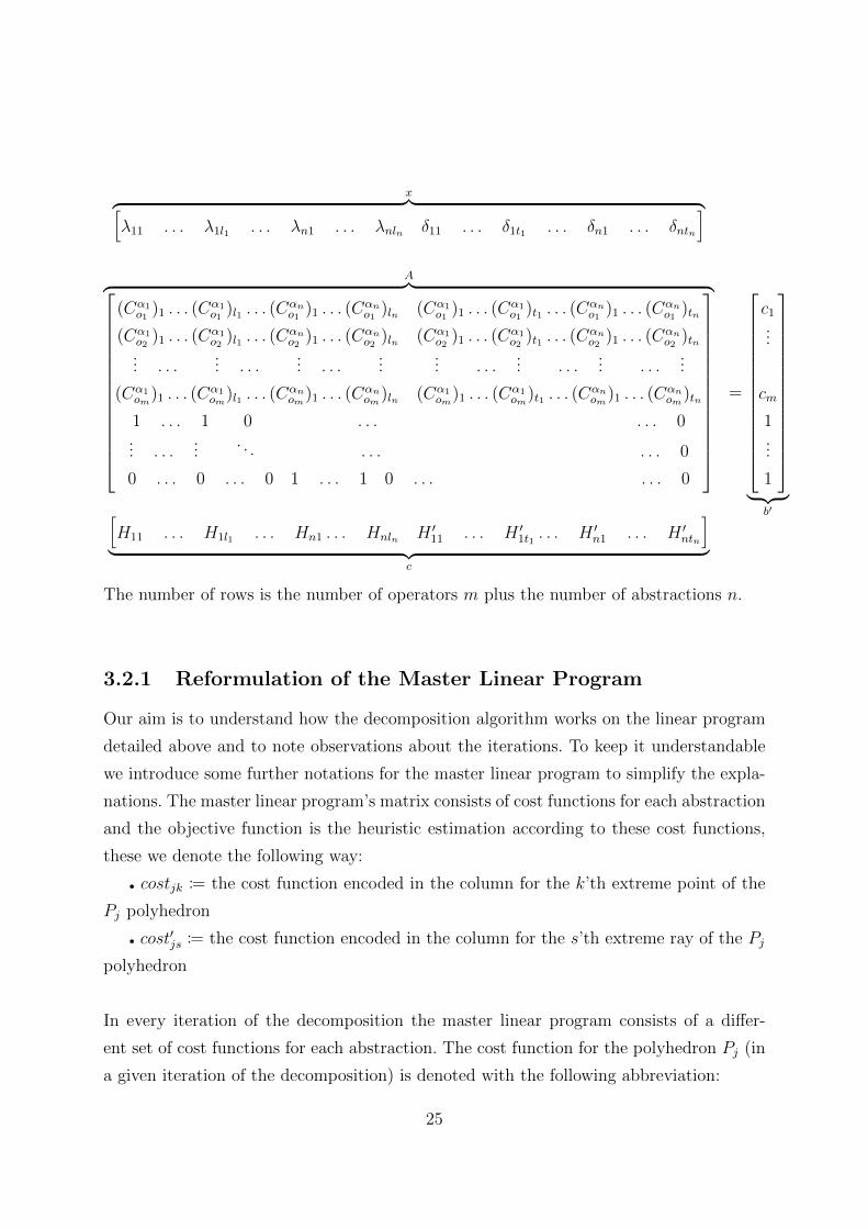
The number of rows is the number of operators m plus the number of abstractions n.

3.2.1 Reformulation of the Master Linear Program

Our aim is to understand how the decomposition algorithm works on the linear program

detailed above and to note observations about the iterations. To keep it understandable

we introduce some further notations for the master linear program to simplify the expla-

nations. The master linear program’s matrix consists of cost functions for each abstraction

and the objective function is the heuristic estimation according to these cost functions,

these we denote the following way:

• costjk := the cost function encoded in the column for the k’th extreme point of the

Pj polyhedron

• cost′js := the cost function encoded in the column for the s’th extreme ray of the Pj

polyhedron

In every iteration of the decomposition the master linear program consists of a differ-

ent set of cost functions for each abstraction. The cost function for the polyhedron Pj (in

a given iteration of the decomposition) is denoted with the following abbreviation:

25

• costj :=∑

k,s

(λjkcostjk + δjscost

′js

)k = 1, 2, . . . , lj s = 1, 2, . . . , tj (We consider

only the extreme points and rays appearing in the current iteration.)

We denoted by Hjk and H ′js the coordinates belonging to the abstract goal state in the

cost functions costjk and cost′js for abstractin αj. Let us express the heuristic estimation

belonging to the αj abstraction in the current iteration of the decomposition algorithm

as a result of the following observations.

We know from the definition of the subproblems that

• h(costjk) = Hjk

and h(costjs) = H ′js.

For any abstraction heuristic h, any two cost functions cost1, cost2, and any non-negative

real number x we have

• h(cost1) + h(cost2) = h(cost1 + cost2) and

• x ∗ h(cost1) = h(x ∗ cost1).This is because abstraction heuristics are linear functions when seen as functions of the

operator cost vectors.

As a result of the observations above the heuristic estimation belonging to the αj

abstraction is hαj =∑

k λjkHjk +∑

s δjsH′js.

The simplified master linear program with these new notations:

maximize∑j

hαj

subject to∑j

costj(o) ≤ cost(o) ∀o ∈ O

hαj =∑

k λjkHjk +∑

s δjsH′js ∀k = 1, 2, . . . , lj s = 1, 2, . . . , tj∑

k

λjk = 1 ∀αj ∈ A

After elaborating the details we can see what the Dantzig-Wolfe decomposition com-

putes when solving the linear program for cost partitioning: In each iteration it computes

a cost vector and an associated heuristic value. The master linear program takes these

vectors and builds a linear combination of them for each abstraction. It then combines

these linear combinations by cost partitioning in an optimal way.

26

3.3 An Iteration of the Decomposition Algorithm

In this section, we will analyze the steps of the Dantzig-Wolfe decomposition algorithm

applied on the linear program for cost partitioning.

In the first stage of the DW algorithm, we need a basis of the master problem’s matrix.

This means, that we need m+ n cost functions, at least one for each abstraction and the

cost functions belonging to one abstraction have to be linearly independent as vectors.

To obtain a collection of cost functions like this we can repeatedly call an LP solver for

the Pj polyhedrons with an arbitrary target function. One call will give us an extreme

point or an extreme ray of the given polyhedron, and we add the resulting vector to our

collection if it is linearly independent from the vectors already added to the collection.

The computation of this start basis is exhaustive, this is why we chose a different approach

in practice.

We start with the identity matrix as start basis. In this case the start basis columns are

not related to the original problem, but they give a valid initial solution to the problem,

namely the zero vector. This is the start basis we use in the experiments. These columns

do not have cost in the master linear program and they do not assign cost to operators,

they are just helping the initialization.

Let us denote the gained basis by B. The equality Bx = b′ has a unique solution,

x = B−1b′. This is a non-negative vector, so we have a primal-feasible solution.

To determine, if x is an optimal solution, we have to examine the dual problem:

Let us denote the dual problem’s variables by (y, z), where y refers to the operator cost

constraints, z refer on the constraints expressing∑

i λji = 1. The dual problem:

minimize b′(y, z)

subject to (y, z)TA ≥ c

According to the duality theorem, if the basis B is dual-feasible too, then the current

x is an optimal solution for the linear program.

Let us denote by cB the sub-vector of c under the basis coordinates. The value of the

dual solution can be also uniquely calculated by the equation (y, z)TB = cB.

Let us pick any column of the master problem and denote the corresponding cost

function costjk by C and its heuristic estimation H in case of an extreme point, or H ′ if

the cost function is an extreme ray of the polyhedron Pj. To check the dual-feasibility we

have to verify, that for every column of A the inequality yTC + zj ≥ H is true (in the

27

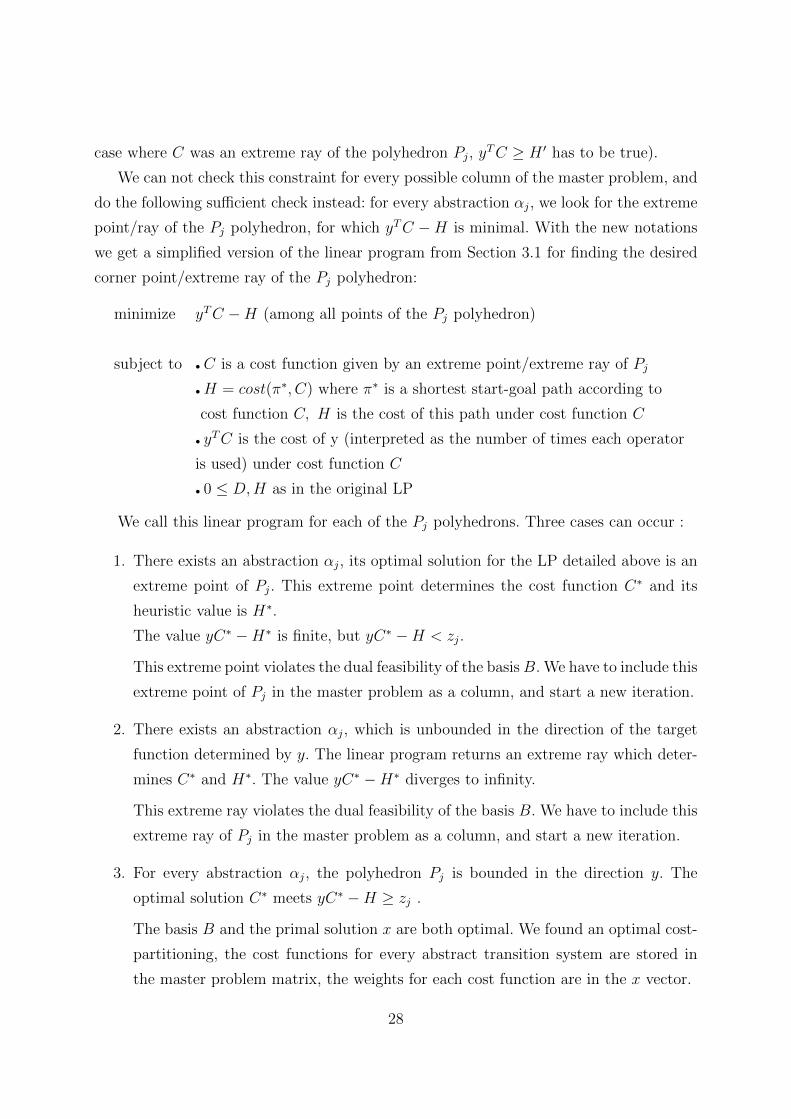
case where C was an extreme ray of the polyhedron Pj, yTC ≥ H ′ has to be true).

We can not check this constraint for every possible column of the master problem, and

do the following sufficient check instead: for every abstraction αj, we look for the extreme

point/ray of the Pj polyhedron, for which yTC −H is minimal. With the new notations

we get a simplified version of the linear program from Section 3.1 for finding the desired

corner point/extreme ray of the Pj polyhedron:

minimize yTC −H (among all points of the Pj polyhedron)

subject to •C is a cost function given by an extreme point/extreme ray of Pj

•H = cost(π∗, C) where π∗ is a shortest start-goal path according to

cost function C, H is the cost of this path under cost function C

• yTC is the cost of y (interpreted as the number of times each operator

is used) under cost function C

• 0 ≤ D,H as in the original LP

We call this linear program for each of the Pj polyhedrons. Three cases can occur :

1. There exists an abstraction αj, its optimal solution for the LP detailed above is an

extreme point of Pj. This extreme point determines the cost function C∗ and its

heuristic value is H∗.

The value yC∗ −H∗ is finite, but yC∗ −H < zj.

This extreme point violates the dual feasibility of the basisB. We have to include this

extreme point of Pj in the master problem as a column, and start a new iteration.

2. There exists an abstraction αj, which is unbounded in the direction of the target

function determined by y. The linear program returns an extreme ray which deter-

mines C∗ and H∗. The value yC∗ −H∗ diverges to infinity.

This extreme ray violates the dual feasibility of the basis B. We have to include this

extreme ray of Pj in the master problem as a column, and start a new iteration.

3. For every abstraction αj, the polyhedron Pj is bounded in the direction y. The

optimal solution C∗ meets yC∗ −H ≥ zj .

The basis B and the primal solution x are both optimal. We found an optimal cost-

partitioning, the cost functions for every abstract transition system are stored in

the master problem matrix, the weights for each cost function are in the x vector.

28

We repeatedly call the master linear program. If case 1. or case 2. occures, we ex-

tend the master LP and re-solve the problem. If case 3 occures, we got the optimal cost

partitioning and we can reconstruct the plan from the master linear program. We now

illustrate the method on the miconic example.

3.3.1 Running the Algorithm on the Miconic Example

The linear program for finding the optimal cost partitioning for the miconic example is

maximize cTx

subject to Ax ≤ b,

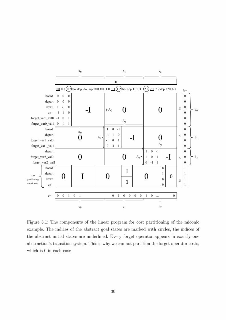
as illustrated in Figure 3.1. The desired x has to be 0 at the coordinates belong-

ing to abstract initial states and non-negative at every abstract state coordinate. Solv-

ing this linear program with any LP solver gives us the following optimal result: x∗ =

[0, 0, 0, 0, 0, 0, 0, 0, 0, 1, 0, 0, 1,−1, 0, 0, 2, 0, 0, 2, 0, 0], which means:

• We assign cost 0 to the operators up and down in α0

• We assign cost 1 to the operator board and cost −1 to the operator depart in α1

• We assign cost 2 to the operator depart in α2

and this results cTx∗ = 2.

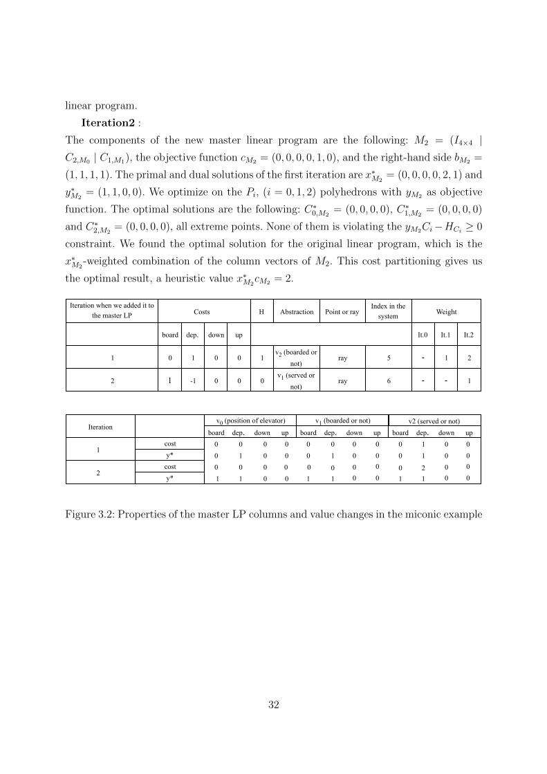
Let us see how the the decomposition algorithm for solves the same linear program.

Figure 3.2 summarizes the changes during the algorithm.

Initialization :

The miconic example has 3 state variables and 4 transitions. After normalizing the task

and creating the atomic abstractions the result is 3 abstractions, α0, α1 and α2 illustrated

on Figure 2.2. To each αi abstraction (i = 0, 1, 2) belongs a polyhedron Pi = {xi : Aixi ≤bi, xi ≥ 0} according to Figure 3.1. These are the polyhedrons we will optimize with

changing objective function in every iteration.

First we initialize the columns of the master linear program as a start base M0 = I4×4,

the objective function cM0 = (0, 0, 0, 0), and the right-hand side bM0 = (1, 1, 1, 1). In the

i ’th iteration of the decomposition algorithm, we are going to solve the linear program

maximize cTMixMi

subject to MixMi≤ bMi

, xMi≥ 0,

29

0.0 0.1 0.2 bo. dep. do. up f00 f01 bo.1.0 1.1 1.2 2.0 2.1 2.2dep. dep.f10 f11 f20 f21

-I

-I

-I

0 0

0 0

00

-1

-1

-1

-11

1

1

1

1

1

1

1

-1

-1

-1

-1

x

1

1

1

-1

-1

-1

1

c=

0

00

0

0

0

0

0

0

0

0

0

0

0 0 0

0 0

0

0

0

0

0

0

0

0

0

0

0

0

≤

≤

≤

≤

1

1

1

1

board

depart

down

forget_var0_val0

forget_var0_val1

up

board

depart

forget_var1_val0 

forget_var1_val1

depart

forget_var2_val0 

forget_var2_val1

board

depart

down

up

b=

b0

b1

b2

x0 x1 x2

A0

A1

A2

costpartitioningconstraints

A0

A1

A2

1 1 10 0 0 0 0 00 00 0... ...

c0 c1 c2

0 I 0I

00

00

00

Figure 3.1: The components of the linear program for cost partitioning of the miconic

example. The indices of the abstract goal states are marked with circles, the indices of

the abstract initial states are underlined. Every forget operator appears in exactly one

abstraction’s transition system. This is why we can not partition the forget operator costs,

which is 0 in each case.

30

where after each iteration the Mi matrix will have one more column, the x and c vectors

will have one more coordinate. The primal solution in the 0’th iteration is x∗M0= (0, 0, 0, 0).

This solution does not have an interpretation, since it belongs to the starter columns, the

identity vectors. The dual linear program in the i ’th iteration is

minimize bTMiyMi

subject to MTi yMi

≥ cMi, yMi

≥ 0,

The solution of the dual LP in the initialization step is y∗M0= (0, 0, 0, 0). With this

(artificial) dual solution we can start the iterations of the decomposition algorithm. We

have to test if this solution of the master LP is an optimal solution for the whole LP with

optimizing on the three polyhedrons:

minimize yM0Ci −HCi

subject to Ci ∈ PiThe optimal solutions assign costs to the operators (board, depart, down, up) in the

following way: C∗0,M0= (0, 0, 0, 0), C∗1,M0

= (0, 0, 0, 0) and C∗2,M0= (0, 1, 0, 0), where the

first two are extreme points, the last one is an extreme ray. C∗2,M0assigns cost 1 to the

depart operator in the second abstraction. This is a violating cost function C∗2,M0, since

the abstract start-goal shortest path in the transition system of α2 costs 1 so yM0C∗2,M0−

HC∗2,M0= 0− 1 = −1 < 0. This is why solution xM0 is not optimal for the original LP. We

also see, that using no operators (as defined in y∗M0) would cost 0 but this cost function

shows you can get a heuristic value of 1 if you use one of them. We have to include this

violating extreme ray as a column in the master linear program and we complement the

objective function with HC∗2,M0.

Iteration1 :

The components of the new master linear program are the following: M1 = (I4×4 | C2,M0),

the objective function cM1 = (0, 0, 0, 0, 1), and the right-hand side bM1 = (1, 1, 1, 1). The

primal and dual solutions of the first iteration are x∗M1= (0, 0, 0, 0, 1) and y∗M1

= (0, 1, 0, 0).

We optimize on the Pi, (i = 0, 1, 2) polyhedrons with yM1 as objective function. The

optimal solutions are the following: C∗0,M1= (0, 0, 0, 0) extreme point of P0, C

∗1,M1

=

(1,−1, 0, 0) extreme ray of P1 and C∗2,M1= (0, 0, 0, 0) extreme point of P2. There is a

violating cost function C∗1,M1, since the shortest path in the transition system of α1 costs

0 so yM1C∗1,M1− HC∗1,M1

= −1 + 0 = −1 < 0. The solution xM1 is not optimal for the

original LP. We have to include this violating extreme ray as a column in the master

31

linear program.

Iteration2 :

The components of the new master linear program are the following: M2 = (I4×4 |C2,M0 | C1,M1), the objective function cM2 = (0, 0, 0, 0, 1, 0), and the right-hand side bM2 =

(1, 1, 1, 1). The primal and dual solutions of the first iteration are x∗M2= (0, 0, 0, 0, 2, 1) and

y∗M2= (1, 1, 0, 0). We optimize on the Pi, (i = 0, 1, 2) polyhedrons with yM2 as objective

function. The optimal solutions are the following: C∗0,M2= (0, 0, 0, 0), C∗1,M2

= (0, 0, 0, 0)

and C∗2,M2= (0, 0, 0, 0), all extreme points. None of them is violating the yM2Ci−HCi ≥ 0

constraint. We found the optimal solution for the original linear program, which is the

x∗M2-weighted combination of the column vectors of M2. This cost partitioning gives us

the optimal result, a heuristic value x∗M2cM2 = 2.

IterationwhenweaddedittothemasterLP Costs H Abstraction Pointorray

Indexinthesystem

It.0 It.1 It.2board dep. down up

5

6

- 1 2

- - 1

ray

ray

v2(boardedornot)

v1(servedornot)

Iterationboard dep. down up board dep. down up board dep. down up

costy*costy* 1 1

1

0 0 00 00

0 00 00 00

1 1 1 1

1 10 00 0 0 0

0 0 0 0

0 0 0 0

0 0 0 0

0 0 0

0 00

1

2

Weight

1

2

0 1 0 0

0 0 0

1

-11

1

2

v0(positionofelevator) v1(boardedornot) v2(servedornot)

Figure 3.2: Properties of the master LP columns and value changes in the miconic example

32

Chapter 4

Computational Experiments

We implemented the Dantzig-Wolfe decomposition algorithm to solve the linear program

for optimal cost-partitioning. The details of this experiment and the results are discussed

in this chapter.

4.1 Experimental Setup

For the experiment we built up most of the necessary functions and data analyzing scripts

from scratch in Python 2.7. The planning tasks we test the method on are all tasks from

the optimal tracks of the International Planning Competitions (IPC) 1998−2014. This set

consists of 1667 tasks from 57 domains. The format of the tasks is the Planning Domain

Definition Language (PDDL). PDDL (Fox and Long, 2003) is a standard formalism to

define planning problems. pegso To prepare the planning tasks we use the preprocessor

of the Fast Downward planning system (Helmert, 2006). This preprocessor takes the

planning tasks in PDDL format as input, it parses the data and runs an initial analysis

on them. We used a modified version of the preprocessor that creates transition normal

form and transforms the planning tasks to SAS+ format. After the preprocessing step we

proceed with the parsed, normalized planning tasks in SAS+ format. The Python module

abstractions.py creates the atomic abstractions for the planning tasks which we store in

the memory as abstractions objects. The solve.py module uses these abstraction instances

to create the linear program for each abstraction and it performes the Dantzig-Wolfe

decomposition to find an optimal cost-partitioning for theese abstractions. Throughout

this algorithm, we have to solve several linear optimization instances, for which we use

CPLEX 12.8. Every linear program needed during the experiment is created once and kept

33

in memory. In every iteration of the decomposition algorithm we only change the objective

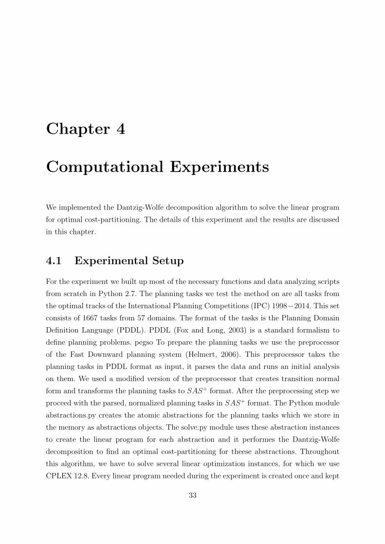
function of these initially constructed linear programs. The workflow is summarized on

Figure 4.1.

PDDLplanningtasks

NormalizedSAS+tasksinTNF

Abstractionobjects

Linearprograms

Optimalcostpartitioningfortheabstractions

HeuristicsearchPreprocessorofFast

Downwardabstractions.py

solve.py

Figure 4.1: Experiment workflow. The heuristic value calculated with the decomposition

method can be used as an admissible heuristic function for solving planning tasks with

heuristic search.

The experiments were executed on a cluster of machines at the Computer Science

Department of the University of Basel. The cluster consists of 24 nodes with 16 cores

each. Every task of the experiment was limited to a single core. Each task had memory

limit 3833 MB, the running time limit was 6000 seconds.

To verify the correctness and to analyse the performance of the decomposition algo-

rithm for cost partitioning, we implemented a Python program lpsolver.py to solve the

whole linear program for cost partitioning without decomposition. We ran the experiments

for lpsolver.py with the same conditions and preprocessing steps detailed above.

4.2 Experiment Results and Analysis

The implemented method (solve.py) successfully solves the linear programs for cost parti-

tioning with the Dantzing-Wolfe decomposition. After running the algorithm on the 1667

planning tasks

• 923 tasks finished with the optimal solution for the cost partitioning LP and were

included in the analysis

• 167 exceeded the time limit, so they only reached an approximating result due to

the time limit we set

34

• 452 tasks exceeded the memory limit

• 125 tasks finished within time and memory, but were excluded from the analysis

for various reasons (they were uncomparable with the results of lpsolver.py, or they

had rounding inaccuracy)

• In 174 cases we could compute the optimal cost partitioning with the Dantzig-

Wolfe decomposition while the full LP solver could not solve the task within the

same resource limits.

The significant amount of uncompleted experiments is not surprising: the set of plan-

ning tasks we are testing on contains many complex tasks with high memory need on

purpose. The proportion of completed tasks can be enhanced with extending the time

and memory limits, using a different programming language, optimizing the data struc-

tures and basic functions in the program. However, the number of successfully completed

instances is still high enough to give a comprehensive analysis on the method. Further-

more, the uncompleted experiments emphasize the weak points of the method which lets

us analyse the performance of the method from a different point of view.

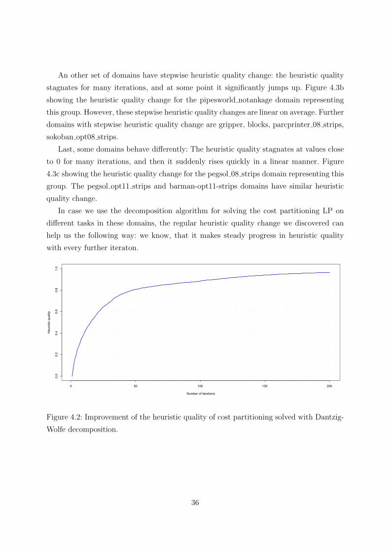
4.2.1 Heuristic Quality

During the iterations of the decomposition algorithm the heuristic value h is monotonously

raising until it reaches the optimal solution for cost partitioning, h∗. To learn more about

the behavoir or the decomposition algorithm, we calculated and visualized the ratio of

these values in every iteration: h/h∗ is the heuristic quality. On Figure 4.2 we can see

the geometric mean of the heuristic quality change for all completed experiments over 200

iterations. The heuristic quality increases steeply in the first few iterations, and with 50 it-

erations the average heuristic quality exceeds 0.8 accuracy. This graph tells us information

about the set of the tasks we tested with: most of the tasks got the final heuristic value

within 50 iterations. However, these averaged values hide some interesting phenomenon.

We visualized the heuristic quality change for every single task per domain, creating one

graph for each domain. We looked over these graphs and found the following patterns on

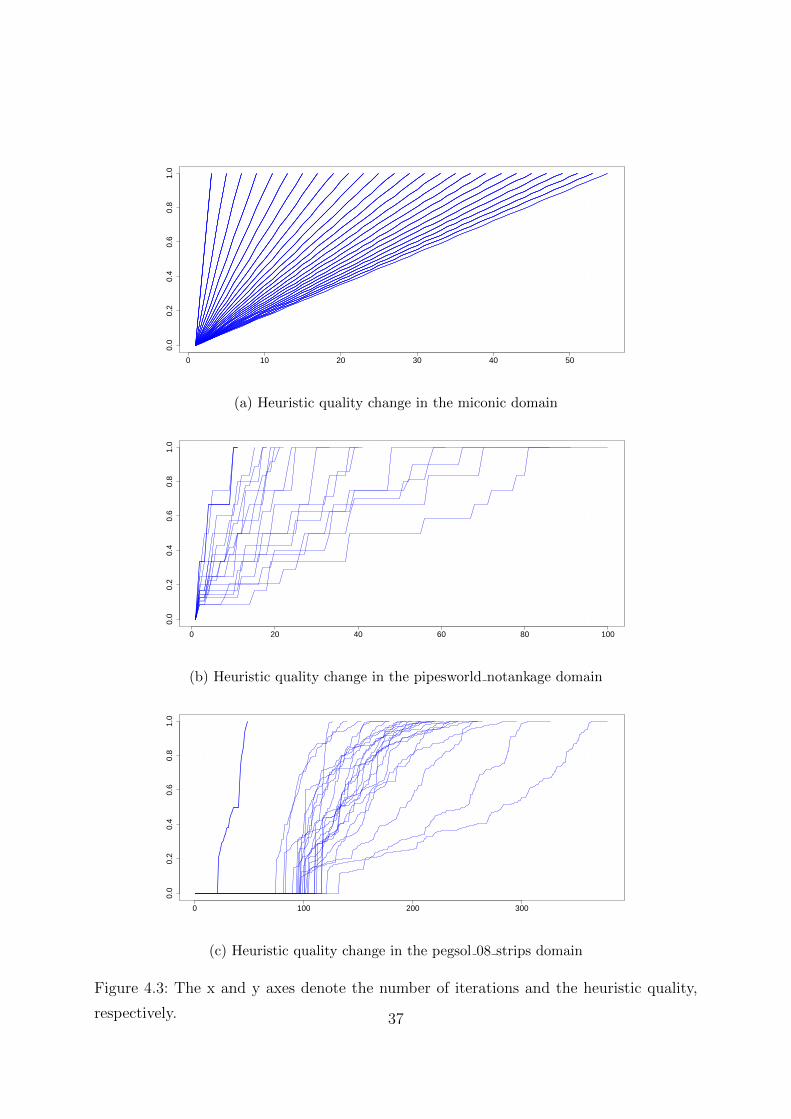
them. A set of domains have precisely linear heuristic quality change. Figure 4.3a showing

the heuristic quality change for the miconic domain representing this group. The rovers,

pathways-noneg, airport and logistics00 domains have similarly linear heuristic quality

change.

35

An other set of domains have stepwise heuristic quality change: the heuristic quality

stagnates for many iterations, and at some point it significantly jumps up. Figure 4.3b

showing the heuristic quality change for the pipesworld notankage domain representing

this group. However, these stepwise heuristic quality changes are linear on average. Further

domains with stepwise heuristic quality change are gripper, blocks, parcprinter 08 strips,

sokoban opt08 strips.

Last, some domains behave differently: The heuristic quality stagnates at values close

to 0 for many iterations, and then it suddenly rises quickly in a linear manner. Figure

4.3c showing the heuristic quality change for the pegsol 08 strips domain representing this

group. The pegsol opt11 strips and barman-opt11-strips domains have similar heuristic

quality change.

In case we use the decomposition algorithm for solving the cost partitioning LP on

different tasks in these domains, the regular heuristic quality change we discovered can

help us the following way: we know, that it makes steady progress in heuristic quality

with every further iteraton.

0 50 100 150 200

0.0

0.2

0.4

0.6

0.8

1.0

Average heuristic quality change in maximum 200 iterations

Number of iterations

Heu

ristic

qua

lity

Figure 4.2: Improvement of the heuristic quality of cost partitioning solved with Dantzig-

Wolfe decomposition.

36

0 10 20 30 40 50

0.0

0.2

0.4

0.6

0.8

1.0

(a) Heuristic quality change in the miconic domain

0 20 40 60 80 100

0.0

0.2

0.4

0.6

0.8

1.0

(b) Heuristic quality change in the pipesworld notankage domain

0 100 200 300

0.0

0.2

0.4

0.6

0.8

1.0

(c) Heuristic quality change in the pegsol 08 strips domain

Figure 4.3: The x and y axes denote the number of iterations and the heuristic quality,

respectively. 37

4.2.2 Running Time and Memory Usage

With the Dantzig-Wolfe decomposition algorithm we would like to solve the linear program

for cost partitioning in a more effective way. To verify the performance of the algorithm, it

is essential to investigate how long it took to compute the optimum with the decomposition

algorithm, and compare it with other methods. This is why we implemented the lpsolver.py

function, which solves the linear program for cost partitioning by solving the whole linear

program.

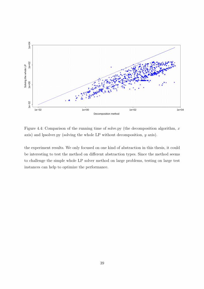
As a result, we did not get the desired running time improvement: solving the linear

program with the decomposition algorithm takes significantly longer than getting the

solution by solving the whole LP, as we can see on Figure 4.4. However, the graph also

shows that in case we would like to solve more complex problems, the difference between

the running time of the two methods gets closer. This is why we suspect, that at highly

complex instances the decomposition algorithm could lead to the final result quicker.

The other factor we would like to improve with the decomposition algorithm is the

memory usage: we are hoping to use less memory with decomposing the linear program

into subproblems and solving smaller linear programs multiple times. The experiment to

solve the whole linear programs for cost partitioning with the lpsolver.py function brought

the following results: it calculated 1042 tasks correctly, furthermore it finished 625 times

with exceeding the memory limit out of 1667 tasks. This is where the strength of the

Dantzig-Wolfe decomposition shows up: at 174 tasks memory error occured when solving

the whole linear program, but the decomposition algorithm could handle these tasks with

the same memory limit. The Dantzig-Wolfe decomposition is suitable for handling complex

tasks when applying it to solve the linear program for cost partitioning.

4.2.3 Conclusion and Future Work

The Dantzig-Wolfe decomposition is a promising tool for solving the linear program for

cost partitioning. The experiments have shown several surprising patterns in the behavoir

of the decomposition method for the cost partitioning LP. In most of the iterations when

optimizing on the subpolyhedrons, we get an extreme ray to extend the master LP with

it. Despite of this the algorithm runs in finite time and it approaches the optimum in a

linear way in practice. The evenness of the heuristic quality increase is unexpected: such

regular behavoir lets us suspect that the method is worth further investigation. Choosing

an appropriate programming language and algorithm-fitted data structures could improve

38

1e−02 1e+00 1e+02 1e+04

1e−

021e

+00

1e+

021e

+04

Decomposition method

Sol

ving

the

who

le L

P

Figure 4.4: Comparison of the running time of solve.py (the decomposition algorithm, x

axis) and lpsolver.py (solving the whole LP without decomposition, y axis).

the experiment results. We only focused on one kind of abstraction in this thesis, it could

be interesting to test the method on different abstraction types. Since the method seems

to challenge the simple whole LP solver method on large problems, testing on large test

instances can help to optimize the performance.

39

Bibliography

Christer Backstrom and Bernhard Nebel. Complexity results for SAS+ planning. Com-

putational Intelligence, 11:625–655, 1993.

Dantzig. Maximization of linear function of variables subject to linear inequalities. Ac-

tivity Analysis of Production and Allocation. Proceedings of the Conference on Linear

Programming, 1951.

George B. Dantzig and Philip Wolfe. Decomposition principle for linear programs. Oper-

ations Research, 1960.

Edsger W. Dijkstra. A note on two problems in connexion with graphs. Numerische

Mathematik, 1(1):269–271, 1959.

Lester R. Ford and Delbert R. Fulkerson. A suggested computation for maximal multi-

commodity network flows. Management Science, 1958.

Maria Fox and Derek Long. PDDL2.1: An extension to PDDL for expressing temporal

planning domains. Journal of Artificial Intelligence Research, 20:61–124, 2003.

Valentina Halasi. Polynomial linear programming methods. Master’s thesis, University

Eotvos Lorand, 2016.

Peter E. Hart, Nils J. Nilsson, and Bertram Raphael. A formal basis for the heuristic

determination of minimum cost paths. IEEE Transactions on Systems Science and

Cybernetics, SSC-4(2):100–107, 1968.

Malte Helmert. The Fast Downward planning system. Journal of Artificial Intelligence

Research, 26:191–246, 2006.

40

Michael Katz and Carmel Domshlak. Structural patterns heuristics: Basic idea and con-

crete instance. In ICAPS 2007 Workshop on Heuristics for Domain-Independent Plan-

ning: Progress, Ideas, Limitations, Challenges., 2007.

Michael Katz and Carmel Domshlak. Optimal additive composition of abstraction-based

admissible heuristics. In Proceedings of the Eighteenth International Conference on

Automated Planning and Scheduling, ICAPS, 2008.

Michael Katz and Carmel Domshlak. Optimal admissible composition of abstraction

heuristics. Artificial Intelligence Journal, 174(12–13):767–798, 2010.

L. G. Khachiyan. A polynomial algorithm in linear programming (in russian). Doklady

Akademii Nauk SSSR, 1979.

H. Minkowski. Allgemeine Lehrsatze uber die konvexen Polyeder. Nachrichten von der

Gesellschaft der Wissenschaften zu Gottingen, 1897.

Neumann. Discussion of a maximum problem. unpublished working paper, Institute for

Advanced Study, Princeton, 1947. Reprinted in: John von Neumann, Collected Works,

Vol. VI (A. H. Taub, ed.), Pergamon Press, Oxford, 1963, pp. 89-95.

Judea Pearl. Heuristics: Intelligent search strategies for computer problem solving.

Addison-Wesley, 1984.

Florian Pommerening and Malte Helmert. A normal form for classical planning tasks.

Proceedings of the Twenty-Fifth International Conference on Automated Planning and

Scheduling (ICAPS), pages 188–192, 2015.

Florian Pommerening, Malte Helmert, Gabriele Roger, and Jendrik Seipp. From non-

negative to general operator cost partitioning. In Proceedings of the Twenty-Ninth

AAAI Conference on Artificial Intelligence, pages 3335–3341, 2015.

Gabriele Roger and Florian Pommerening. Linear programming for heuristics in opti-

mal planning. In Proceedings of the AAAI-2015 Workshop on Planning, Search, and

Optimization (PlanSOpt), 2015.

Alexander Schrijver. Theory of linear and integer programming. John Wiley & Sons, 1999.

H. Weyl. Elementare Theorie der konvexen Polyeder. Commentarii Mathematici Helvetici,

1935.

41

Fan Yang, Joseph C. Culberson, Robert Holte, Uzi Zahavi, and Ariel Felner. A general

theory of additive state space abstractions. Journal of Artificial Intelligence Research,

32:631–662, 2008.

42