______________________________________________________________________________ 6001 Shellmound St., Suite 700 Emeryville, California 94608-1954 USA Tel: (510) 655-7400 Fax: (510) 655-9517

June 7, 2002 Dr. Stephen DiZio Chief (Acting) Human and Ecological Risk Division 8810 Cal Center Drive, Second Floor Sacramento, CA 95826 Dear Steve: On behalf of PG&E and the US Navy, we are submitting an electronic copy for your review of the report, “Background Levels of Polycyclic Aromatic Hydrocarbons in Northern California Surface Soil”. In addition to the main text of the report, we have attached a copy of Appendix A, which is a printed copy of the Final Data Base, and Appendix B, which is an electronic copy of the complete PAH database. Per your request, we will also send you two printed copies of the complete report. The printed copies will include Appendix C, which is a copy of the lab sheets for the data included in the database. This Appendix, less the newer DTSC data from Midway Village, was previously submitted to you and others at DTSC on January 31, 2001 (Memorandum from Wini Curley and Daphne Chong, Entrix, to Northern California Background Study Team, Re: Data Packages and Initial PG & E Database). I would be happy to send a printed copy of the report to anyone on your review team who calls me at (510) 420-2551 to request one. We will contact you next week after you have had a chance to identify your DTSC review team and to check with their schedules to arrange a date to discuss your comments. We look forward to meeting with you and your review team to discuss your comments and the peer review process. Sincerely,

Robert Scofield, D.Env. Principal Attachments (2)

• Report: “Background Levels of Polycyclic Aromatic Hydrocarbons in Northern

• Data diskette Y:\USN\USN Letter 060702.doc

BACKGROUND LEVELS OF POLYCYLIC

AROMATIC HYDROCARBONS IN NORTHERN CALIFORNIA SURFACE SOIL

Prepared for:

Pacific Gas and Electric Company and

U.S. Navy

Prepared by: ENVIRON Corporation

ENTRIX IRIS Environmental

and ENV America

June 7, 2002

03-9166B and 03-9497A

i June 7, 2002

TABLE OF CONTENTS

EXECUTIVE SUMMARY .........................................................................................................E-1

1.0 INTRODUCTION ...........................................................................................................1-1

1.1 Purpose and Objectives ................................................................................................1-2

1.2 Document Organization...............................................................................................1-2

2.0 OVERVIEW OF DATA SET DEVELOPMENT AND STATISTICAL METHODOLOGY...........................................................................................................2-1

2.1 Overview of the Data Set Development Process .........................................................2-1

2.1.1 Phase 1: Acquisition and Compilation of Initial Data and Development of the Interim Data Set ...................................................................................................................2-1

2.1.2 Phase 2: Evaluation of the Interim Data Set and Development of the Final Data Set.......................................................................................................................2-2

2.1.3 Phase 3: Evaluation of the Final Data Set...............................................................2-3

2.2 Statistical and Graphical Methods Used to Develop the Data Set ...............................2-3

2.2.1 Graphical Methods ...................................................................................................2-4

2.2.1.1 Box and Whisker Plots.....................................................................................2-4

2.2.1.2 Scatter Plots......................................................................................................2-5

2.2.1.3 Probability Plots ...............................................................................................2-5

2.2.2 Statistical Calculations Used During the Development of the Data Set..................2-5

2.2.2.1 Summary Statistics...........................................................................................2-5

2.2.2.2 Hypothesis Tests ..............................................................................................2-6

2.2.2.2.1 The Shapiro-Wilk Test for Normality........................................................2-6

2.2.2.2.2 Comparison of Categories: Kruskal-Wallis/Mann-Whitney .....................2-6

3.0 PHASE 1: DEVELOPMENT OF THE INTERIM DATA SET ....................................3-1

3.1 Acquisition of Data and Review for Inclusion in the Initial Data Set .........................3-1

3.1.1 Selection of Data for the Initial Data Set .................................................................3-1

3.1.2 Locations Identified for the Northern California Data Set ......................................3-3

3.2 Criteria for Data Inclusion/Exclusion..........................................................................3-3

4.0 PHASE 2: EVALUATION OF INTERIM DATA SET AND DEVELOPMENT OF THE FINAL DATA SET..........................................................................................................4-1

4.1 Evaluation of the Interim Data Set...............................................................................4-1

4.1.1 Comparisons Among Categories .............................................................................4-2

ii June 7, 2002

4.1.2 Consistency with a Common Distribution...............................................................4-4

4.2 Reduction of Data Points Associated with Midway Village and Redding Sites .........4-5

4.3 Identification of Outliers and Further Reduction of the Interim Data Set ...................4-5

4.4 Treatment of Non-Detects and Elevated Detection Limits..........................................4-5

4.4.1 Significance of Non-Detects and Elevated Detection Limits ..................................4-6

4.4.2 Development of B(a)P Equivalent Concentrations for the Final Data Set ..............4-6

5.0 PHASE 3: EVALUATION OF THE FINAL DATA SET.............................................5-1

5.1 Comparisons Among Categories .................................................................................5-1

5.2 Consistency with a Common Distribution...................................................................5-2

5.3 Development of the Smoothed Data Set......................................................................5-2

6.0 SUMMARY AND CONCLUSIONS ..............................................................................6-1

REFERENCES ........................................................................................................................... R-1

LIST OF TABLES

Table 3.1: Samples Proposed for Exclusion from Initial Data Set Table 4.1: Statistical Summary – Descriptive Statistics B(a)P Equivalents Calculated Using

½ the Reported Detection Limit Interim Data Set Table 4.2: Nonparametric One-Way Analysis of Variance B(a)P Equivalents Calculated

Using ½ the Reported Detection Limit Interim Data Set Table 4.3: List of Sites Categorized by Region Table 4.4: List of Sites Categorized by Proximity to Coast Table 4.5: Samples Proposed for Exclusion from Interim Data Set Table 5.1: Statistical Summary – Descriptive Statistics B(a)P Equivalents Final Data Set

(Unsmoothed) Table 5.2: Nonparametric One-Way Analysis of Variance B(a)P Equivalents Final Data Set

(Unsmoothed) Table 5.3: Summary Statistics for Final Data Set

LIST OF FIGURES

Figure 2.1: Flowchart of Tasks Performed to Construct the 86-Sample Northern California PAH Background Data Set

Figure 2.2: Sample Box and Whisker Plot

iii June 7, 2002

Figure 2.3: Sample Scatterplot Figure 2.4: Sample Probability Plot of Normal Fit to Data Figure 2.5: Sample Probability Plot of Lognormal Fit to Data Figure 3.1: Candidate PG&E and Navy Sites Reviewed for Inclusion in PAH Background

Data Set Figure 4.1: Box and Whisker Plot by Site – 156 Samples Figure 4.2: Box and Whisker Plot by Region – 156 Samples Figure 4.3: Box and Whisker Plot by Proximity to Ocean – 156 Samples Figure 4.4: Scatterplot of B(a)P Equivalent Concentrations versus Number of Detected

Constituents – 156 Samples Figure 4.5: Probability Plot of Normal Fit to Raw Data – 156 Samples Figure 4.6: Probability Plot of Normal Fit to Log Transformed Data – 156 Samples Figure 5.1: Box and Whisker Plot by Site – 86 Samples Figure 5.2: Box and Whisker Plot by Region – 86 Samples Figure 5.3: Box and Whisker Plot by Proximity to Ocean – 86 Samples Figure 5.4: Probability Plot of Normal Fit to Data – 86 Samples Figure 5.5: Probability Plot of Lognormal Fit to Data – 86 Samples Figure 5.6: Probability Plot of Lognormal Fit to Data – 73 Uncensored Samples Figure 5.7: Probability Plot of Lognormal Fit to Data – 86 Samples After Smoothing

APPENDICES Appendix A Printed Copy of Final Data Set

Appendix B Disk with Electronic Copies of Initial, Interim, and Final Data Sets

Appendix C Lab Sheets for Data Considered For or Included in Data Set

E-1 June 7, 2002

EXECUTIVE SUMMARY

This report presents the results of a study commissioned by Pacific Gas and Electric Company (PG&E) and the United States Navy to develop a regional data set of background concentrations of carcinogenic polycyclic aromatic hydrocarbons (CPAHs) in surface soils in northern California. The work was completed by a team of consultants with the cooperation and in consultation with an advisory group of representatives from Cal-EPA’s Department of Toxic Substances Control (DTSC). The primary purpose of this study is to define a single data set of sufficient size and statistical power to accurately characterize the range and distribution of background CPAHs in northern California soils. It is intended that this data set can be used, in conjunction with standard statistical tests applicable to comparisons of background data to site data, to support various investigation and remediation decisions at sites. The impetus for developing such a data base stems from the fact that PAHs are both ubiquitous in the environment and typically occur at higher levels than the cleanup criteria calculated using traditional health risk assessment approaches.

The PAH data used in this study was gathered from previous site investigations in northern California conducted under the DTSC oversight by PG&E and the Navy. Initially, 276 samples from 24 sites were identified as potentially representative of background conditions. These samples were subsequently reviewed and systematically evaluated individually and collectively against a set of criteria designed to determine if they truly represented background conditions. In addition to the set of objective exclusion criteria, various other statistical analyses were conducted to assist in identifying samples that may not be considered representative of typical background conditions in northern California soils. Through an iterative process, samples that were deemed not representative of background were excluded from the data set. Most of the samples excluded from the final data set were removed to correct problems related to elevated detection levels and to avoid over-representation of data collected from any one particular site or local area. The data set was subjected to a series of tests to determine if it represented a single population that can be used throughout northern California or whether sub-populations could be identified that would more appropriately be applied in specific sub-regions. The data was examined using a series of statistical and graphical tests in an attempt to distinguish sub-groups of the population based on several geographic variables. Taken all together, these statistical and graphical tests indicate that the overall variability observed between different sites in the final data set are not related to any identifiable geographical variables and is likely random. These results indicate that the final data set provides a reasonable characterization of the background levels of CPAHs in surface soils in all parts of northern California.

The final data set developed from this study is composed of 86 data points from 21 sites. Results of multiple evaluations demonstrate that the final data set is consistent with a lognormal distribution. Consistency with a lognormal distribution supports the hypothesis that the final background data set represents a single background population. The mean and 95% upper

E-2 June 7, 2002

confidence limit (UCL) of the mean CPAH concentration in the final data set are 0.21 mg/kg and 0.40 mg/kg, respectively, as B(a)P equivalents. The final data set developed in this study provides a practical management tool that can be used to support a variety of site investigation and remediation decisions involving comparisons of background CPAH data to site data.

1-1 June 7, 2002

1.0 INTRODUCTION

This report describes the development of a data set of background concentrations of polycyclic aromatic hydrocarbons (PAHs) in surface soil in northern California. PAHs are found in virtually all surface soil in both rural and urban environments (ATSDR 1999). Their widespread distribution is largely attributable to the fact that there are many natural and anthropogenic sources of PAHs in the environment. Most notably, combustion of fossil fuels, structural fires, and various industrial activities produce PAHs emissions, as do processes such as wild fires and volcanic activity.

This relationship of increased background levels of PAHs to anthropogenic PAH sources is well documented in Jones, et. al. (1989). Since the mid-1800s, samples of surface soils were periodically collected from the Rothamsted Experimental Station, a semi-rural area in southeast England located about 25 miles north of London. The soil samples were collected from a control plot in capped glass jars and stored in a dark room. Jones, et. al. (1989) analyzed the soil samples for PAHs. The results of the study showed a 4-fold increase in PAH concentrations in the surface soil samples between the mid- to late 1800s and 1986. Jones, et. al. (1989) attributed this trend to regional fallout of anthropogenically generated PAHs derived from the combustion of fossil fuels. Similar studies in United States (Van Metre, et. al., 2000) and Antarctica (Mazzera, et. al., 1999) have correlated increased levels of PAHs in sediments and soils to anthropogenic sources, namely the combustion of fossil fuels.

For many sites in California, the range of background concentrations of carcinogenic PAHs (CPAHs) in surface soils is typically higher than the level calculated as corresponding to a lifetime incremental cancer risk of one, or even ten, in a million. This same situation has also been encountered with background soil concentrations of arsenic in California (USEPA 2002). As a matter of practice, the Cal/EPA and USEPA do not require responsible parties to clean sites to levels lower than background for the site related chemicals. When the risk-based action levels for a site related chemical are lower than background levels, and the levels present at the site warrant remediation, the most common risk management approach is to remediate to background levels. However, it is difficult and costly to obtain, on a site-by-site basis, the necessary number of background samples that would be required to conduct meaningful statistical tests with adequate statistical power. Therefore, the development of a regional data set that properly characterizes CPAH background levels and that can be appropriately applied to any site within the region is very advantageous to the efficient, consistent, and expeditious remediation of contaminated sites.

Pacific Gas and Electric Company and the U.S. Navy commissioned this project. The project was conducted in cooperation and collaboration with a task group of representatives from the Human and Ecological Risk Division (HERD) and Site Mitigation branches of the Department of Toxic Substances Control (DTSC), Cal/EPA. The team of consulting firms involved in developing the data base are ENVIRON, Entrix, Iris Environmental, and ENV America.

1-2 June 7, 2002

1.1 Purpose and Objectives

The primary purpose of this study was to identify and characterize a data set of background CPAH concentrations that could be compared to CPAH concentration data collected from individual sites to support various investigation and remediation decisions at these sites. The overall study objectives were as follows:

1. Identify as many previous northern California studies that had collected background PAH data as could practically be obtained and reviewed during the course of the project.

2. From the identified studies, glean all of the available background data and evaluate its suitability to represent background levels of PAHs in northern California.

3. Use statistical tests to characterize the selected background data, thus providing a tool to assist in making the decisions regarding site related CPAH concentrations that typically must be addressed during various phases of site investigations and remediation.

Some of the types of decisions that could be aided by the use of the background data set are: determining the adequacy of the horizontal and vertical delineation of the CPAH impacted area; identifying those areas of the site that should be targeted for remediation; establishing an initial target remediation concentration; determining the scope of the confirmation sampling program; and confirming that the remediation was effective in reducing the concentrations of CPAHs to levels that are representative of background concentrations. It is anticipated that the background data would be used with a variety of graphical techniques and statistical tests applicable to comparisons of background data to site data. An important aspect of the characterization of the background data set was determining whether the data set represented a single population of data from northern California, or if the data set represented two or more sub-regions within northern California.

One of the anticipated benefits from pooling background samples collected from many previously conducted site investigation studies was the creation of one or more background data sets that would be larger than the background data set typically developed for any one site. Having a larger background data set offers the practical benefit of providing a higher level of confidence in what concentrations are representative of background for CPAHs than is discernable from the generally modest number of background samples collected near individual sites. Having a background data set that is representative of all of northern California, or even a sub-region within northern California, also allows a greater degree of consistency between sites for decisions that are made on the basis of background comparisons.

1.2 Document Organization

The introduction to the document is presented in Section 1, including the purpose and objectives and document organization. Section 2 of the report provides an overview of the entire data set development process, and introduces the statistical methods used in evaluating and refining the background data set. The overview includes a description of the various steps taken to identify and characterize the data set in three phases of evaluation. Section 3 of the report describes Phase 1, from the original identification of 276 candidate background samples in the Initial Data Set, through the screening of all samples against a series of exclusion criteria that resulted in the selection of 156 samples for the Interim Data Set. Section 4 of the report describes Phase 2, which is the analysis of the Interim Data Set and the subsequent reduction of samples to the 86

1-3 June 7, 2002

ultimately included in the Final Data Set. Phase 3 is described in Section 5, which presents the evaluation and characterization of the Final Data Set through statistical analyses and a smoothing process. Section 6 presents the summary and conclusions, noting that the Final Data Set is best characterized as representative of a single background population. References are provided in Section 7.

2-1 June 7, 2002

2.0 OVERVIEW OF DATA SET DEVELOPMENT AND STATISTICAL METHODOLOGY

The following Section presents an overview of the entire data set development process and describes the types of statistical analyses conducted during the three different phases of the project. Detailed descriptions of each phase of the development of the background data set, and the specific statistical analyses conducted at each phase, are provided in subsequent sections of this report.

2.1 Overview of the Data Set Development Process

The process of developing the background data set was conducted in three phases. The steps performed in each phase are briefly summarized below. An overview of the data set development process is illustrated in Figure 2.1.

The operations described in this report resulted in the creation of three data sets, all of which are being submitted with this report to DTSC as an Excel workbook (Appendix A). The data sets are referred to below as the Initial Data Set, the Interim Data Set, and the Final Data Set.

The Initial Data Set is a comprehensive, 276-sample data set that includes the CPAH concentration data obtained from all of the samples that were used to characterize background conditions at 24 sites located throughout northern California. The process of compiling the data for the Initial Data Set is described in Section 3 of this report.

A thorough evaluation of the Initial Data Set led to the development of a 156-sample Interim Data Set, which was an interim work product that was further evaluated and reduced to the 86-sample Final Data Set. The Final Data Set was generated by examining the samples in the Interim Data Set and selecting a subset that is considered to be representative of background conditions in the vicinity of PAH-impacted sites in northern California. The PAH concentrations in the samples in the Initial, Interim, and Final Data Sets are characterized by benzo(a)pyrene (B(a)P) equivalent concentration values. The process of generating the Final Data Set from the more comprehensive Interim Data Set is described in Sections 4 and 5 of this report.

2.1.1 Phase 1: Acquisition and Compilation of Initial Data and Development of the Interim Data Set

Phase 1 activities focused on acquiring and compiling available data for PAHs from reports previously prepared under DTSC oversight for PG & E and Navy Sites in northern California and assessing the quality of the information for each data point. The following steps summarize the activities conducted to prepare the spreadsheet entries for the samples included in the Initial Data Set and the initial evaluation of those samples. Steps 1 through 5, described below, summarize the activities conducted as part of Phase 1. Details of Phase 1 activities are provided in Section 3.

2-2 June 7, 2002

Step 1: Inquiries were made of project managers at PG&E, the US Navy and DTSC to identify candidate site reports likely to contain shallow soil data for background PAHs at sites in northern California.

Step 2: Sampling data and relevant descriptive information were extracted from review of the reports for 24 Sites containing PAH data. This effort resulted in compiling the CPAH data from 276 samples into an Excel spreadsheet (referred to as the Initial Data Set). The Initial Data Set, which contains the data from all 276 samples, was generated by calculating the benzo(a)pyrene [B(a)P] equivalent concentration for each sample from the data for the individual CPAHs. For the first two phases of the study, all concentrations reported as non-detects were assigned a concentration of ½ the detection limit.

Step 3: Existing reports and relevant supporting documentation for the 24 sites included in the Initial Data Set were reviewed by the technical team.

Step 4: Four exclusion criteria were developed to identify individual samples that did not qualify as representing background conditions. The codes noted in parenthesis refer to the code assigned to each exclusion criterion in the electronic version of the Initial Data Set submitted with this report. Criteria addressed the following issues: samples collected from depths greater than six inches (Code 1), non-detect data with elevated detection limits for individual CPAHs (Code 2), duplicates or reanalysis of other samples (Code 3), and suspect locations due to proximity to specific sources of PAHs (Code 4).

Step 5: Sample-specific information was reviewed for the 276-samples in the Initial Data Set and the exclusion criteria were applied. The code indicating the basis for eliminating each of the 120 samples removed from the data set at this stage of the process is contained in the Initial Data Set. Deletion of these samples from the Initial Data Set generated the Interim Data Set.

2.1.2 Phase 2: Evaluation of the Interim Data Set and Development of the Final Data Set

Phase 2 focused on further assessing the quality of the information for each sample and determining whether the Interim Data Set, as a whole, is representative of background conditions. A series of statistical tests was used to characterize and refine the Interim Data Set (156 samples) to ultimately yield the Final Data Set of 86 samples. Phase 2 activities are described in detail in Section 4, and consist of Steps 6 through 9, described below:

Step 6: The 156 samples in the Interim Data Set were statistically evaluated to assess whether the overall variability in the concentration of CPAHs could be explained by various sub-sets or categories in the data set (e.g., geographic region). The consistency of the data set with common distributions (normal and lognormal) was also evaluated.

Step 7: A large number of samples were associated with the Midway Village and Redding sites (52 samples and 28 samples, respectively). This resulted in an overrepresentation of those sites in the data set. Therefore, a methodology was

2-3 June 7, 2002

devised in consultation with DTSC to randomly select a reduced number of samples from each of these sites for inclusion in the data set. As a result of the random selection process, a total of 68 samples were excluded (46 samples from Midway Village and 22 samples from Redding).

Step 8: Statistical tests identified two samples as possible outliers at the upper end of the range of B(a)P equivalent concentrations. Inspection of the sampling locations indicated that the high concentrations could potentially be related to contamination from a specific source; therefore, these samples may not be representative of background conditions. Using this exclusion criterion (Code 6), these two samples were removed from the data set to arrive at a Final Data Set of 86 samples.

Step 9: In several of the samples remaining in the data set, one or more of the seven CPAHs were detected, and one or more of the other CPAHs were non-detect with an elevated detection limit (i.e., greater than 0.02 mg/kg). Using a ranking and averaging process, a method was devised to assign values to the non-detect CPAHs with elevated detection limits in order to more accurately estimate the actual B(a)P equivalent concentration for each sample.

2.1.3 Phase 3: Evaluation of the Final Data Set Phase 3 consisted of evaluating and describing the characteristics of the Final Data Set (86 samples). Phase 3 activities are discussed in Section 5, and consist of the following steps:

Step 10: Statistical tests were conducted to characterize the homogeneity of the Final Data Set (86 samples) and its consistency with common distributions.

Step 11: A smoothing process was used to derive better B(a)P equivalent estimates for censored samples identified in the Final Data Set (as described in more detail in Section 4.2.1, censored samples are those in which none of the carcinogenic PAHs was detected). The values obtained by smoothing should be used when calculating important descriptive statistics (mean, standard deviation, etc.).

2.2 Statistical and Graphical Methods Used to Develop the Data Set A number of statistical and graphical analysis methods were used during development and evaluation of the Final Data Set. These tools were used to understand the nature and the distribution of the various data sets and to evaluate their appropriateness to represent background levels of PAH in northern California. Graphical evaluations and statistical analyses were used to identify discrepancies within the data (e.g., to identify deviations from patterns that might suggest the presence of anomalous data points) and between various subgroups of the data; to evaluate the consistency of the data with a normal or lognormal distribution; to summarize the data; and to test hypotheses of equality between the medians of subgroups of the data. Statistical techniques used include graphical analysis (probability plots, box and whisker plots, and scatterplots); summary statistics; and standard hypothesis tests. The analyses were performed with standard statistical tools including Statmost®, SYSTAT®, and Excel®.

2-4 June 7, 2002

2.2.1 Graphical Methods Box and whisker plots, scatterplots, and probability plots were the three general graphical methods used to analyze and visually examine the data. The box and whisker plots provide a nonparametric visual representation of the data. Additionally, the box and whisker plots can be used to visually compare the data distributions within each category. The scatterplots provide a graphical means to compare individual data and observe relationships within the data set. The probability plots provide a graphical method to compare the data to a statistical distribution (e.g., normal or lognormal). Each of these graphical methods is described below.

2.2.1.1 Box and Whisker Plots

Box and Whisker plots were developed for use in identifying outliers and systematic differences or similarities among categories of samples. These plots provide a summary picture of the data distribution for each category (e.g., a different plot for each of North, Central, and South regional categories) allowing a comparison of the differences and similarities among the categories. Figure 2.2 is a sample Box and Whisker plot. The following summarizes the information provided in the plo t

§ The horizontal line within the box represents the median, or 50th percentile value.

§ The rectangular box corresponds to the middle 50 percent of the data; that is, the lower end of the box corresponds to the 25th percentile value (lower hinge) and the upper end of the box corresponds to the 75th percentile value (upper hinge). The difference between these values is referred to as the interquartile range (IQR), and is calculated by subtracting the 25th percentile value from the 75th percentile value.

§ The next expanded range from the 25th and 75th percentile is defined by the inner fences. The upper inner fence is the upper hinge plus 1.5 times the IQR and the lower inner fence is the lower hinge less 1.5 times the IQR.

§ The end of the whiskers (vertical line) coming out of the bottom box is the lowest value that lies between the lower hinge (25th percentile) and the lower inner fence. The end of the whisker coming out of the top of the box is the highest value that lies between the upper hinge (75th percentile) and the upper inner fence.

§ The next expanded range is defined by the outer fences. Subtracting another 1.5 times the IQR from the lower inner fence establishes the lower outer fence (3 times IQR from the hinge). Similarly, adding another 1.5 times the IQR to the upper inner fence establishes the upper outer fence.

§ The asterisks represent individual data points with values that lie between the inner and outer fences.

2-5 June 7, 2002

§ Circles represent individual data points with values that are greater than the upper outer fence or less than the lower outer fence - values greater the 3 times IQR from the hinges.

2.2.1.2 Scatter Plots

Scatter plots allow the observation of trends and relationships between concentration and the various categories. An example is Figure 2.3, which depicts the relationship between the concentration in B(a)P equivalents (plotted in a logarithmic scale) and the number of carcinogenic PAHs detected in each sample. Note that the data do not line up directly above the ordinals indicating the number of detects. For convenience, a jitter or random offset is included in the plot when data points overlap exactly. This allows the observer to see the number of data at each plotting point, rather than a single symbol that may represent multiple data points.

2.2.1.3 Probability Plots

Graphing the data on probability plots (p-plots) allows a direct visual comparison between the frequency distribution of the data and a specific distribution type (e.g., lognormal). The probability plots compare the individual data value to the expected value of the data point assuming a specified distribution. If a linear or near- linear relationship (straight line) is observed, the data are assumed to fit the distribution. We plotted the B(a)P equivalent data against the expected values assuming and testing for a normal distribution. Additionally, the data were plotted on a log scale to test for a lognormal distribution. Data that deviated from the linear relationship were identified as potentially anomalous and were subject to additional review. Examples of normal and lognormal probability plots are presented in Figures 2.4 and 2.5, respectively.

2.2.2 Statistical Calculations Used During the Development of the Data Set

Two types of statistics were calculated throughout the development of the data set and were used to assess and describe its overall characteristics: summary statistics and hypothesis tests. Each type is described below.

2.2.2.1 Summary Statistics

Summary statistics are used to quantify the characteristics of a data set. Important summary statistics include the number of samples, the minimum and maximum values, the average, and the standard deviation. In some cases, the skewness (which describes the symmetry of the data) is also calculated. These statistics provide a numerical description of the data set. Other statistics, such as the coefficient of variation, can be calculated from these basic summary statistics. In addition, the summary statistics of a data set can be used to test certain hypotheses about the population represented by the data set.

2-6 June 7, 2002

2.2.2.2 Hypothesis Tests

Statistical hypothesis tests are used in this study to examine the distributions of the populations represented by the data sets and the significance of differences among the medians of various categories. Tests of consistency with the normal and lognormal distributions were performed using the Shapiro-Wilk test. Hypotheses concerning the equality of medians were tested using nonparametric procedures based on ranks (the Mann-Whitney test for comparing two categories, and the Kruskal-Wallis test for comparing more than two categories). Statistical hypothesis testing involves making an assumption or hypothesis about the population that is represented by the sample data, then evaluating whether the sample data are consistent with the hypothesis (e.g., do sites in the southern portion of the PG&E service area have different concentrations than sites in the northern part of the service area?). The results of a hypothesis test are a quantification of the probability that the population represented by the sample data fits the assumption. If the probability is small (i.e., if the sample data are not consistent with the assumption), the hypothesis is rejected. Otherwise, the hypothesis is not rejected.

For this study, the critical probability used in evaluating the hypothesis tests was five percent (0.05). The results of the statistical tests performed in this study are presented as p-values, which are compared to the five percent (0.05) critical value. If a p-value is less than the critical value of 0.05, then the hypothesis is rejected. The specific hypothesis tests used in this study are briefly summarized below.

2.2.2.2.1 The Shapiro-Wilk Test for Normality

The test for normality assumes a normal distribution and calculates the W (Shapiro-Wilk) statistic from the sample data. If the calculated value of the W statistic has a probability of occurring of less than five percent under the assumption of normality, then the data are considered not normal – the hypothesis is rejected. The test for lognormality is performed by using the Shapiro-Wilk procedure to test the normality of the logarithms of the data set. If the logarithms are not normally distributed, then the hypothesis that the data are representative of a lognormally-distributed population is rejected.

2.2.2.2.2 Comparison of Categories: Kruskal-Wallis/Mann-Whitney

Comparisons of central tendency among categories were performed using nonparametric tests based on ranks. These tests were used to determine whether a significant portion of the variation in the data set can be explained by categorical variables such as the region of northern California in which a site is located. Nonparametric tests were used because the amount of data available in some categories was not sufficient to allow meaningful tests of the assumptions required for parametric tests. The Mann-Whitney test was used for comparing two categories, and the Kruskal-Wallis test was used for comparing more than two categories. These nonparametric tests evaluate the significance of differences among the median values of various categories.

June 7, 2002 3-1

3.0 PHASE 1: DEVELOPMENT OF THE INTERIM DATA SET The purpose of this section is to describe the process used to acquire and review data for inclusion in the Interim Data Set for the northern California study of background soil concentrations for carcinogenic PAHs. The following sections describe the activities conducted to identify existing site related reports containing data for background PAHs, and the criteria used to select and exclude samples as candidates to represent background conditions. From the Initial Data Set, consisting of 276 samples, 120 samples were ultimately excluded to yield the Interim Data Set of 156 samples.

3.1 Acquisition of Data and Review for Inclusion in the Initial Data Set

Initial inquiries were made to PG&E, the US Navy, and DTSC regarding candidate sites where sampling of ambient PAHs had already been conducted. The largest amount of useable data was obtained from PG&E. Preliminary Endangerment Assessments (PEAs) had previously been submitted to DTSC for 25 former Manufactured Gas Plant (MGP) sites located in northern California. Some of those sites also had additional background data collected after the PEAs had been completed. Documentation for these sites was obtained for review. The US Navy identified eight sites in the San Francisco Bay area that had available documentation previously submitted to DTSC. The DTSC team members suggested checking with others in their Federal Facilities Group for additional potential sites as candidates. No additional sites were identified for review. However, additional data for one other site (Midway Village) were obtained for inclusion in site data to be evaluated.

3.1.1 Selection of Data for the Initial Data Set

For the 33 sites initially identified as candidates, documentation was obtained from PG&E, the US Navy, and DTSC. Hard copy reports were reviewed, including original data sheets and boring logs, when available. The dates for the studies collected as a result of these inquiries ranged from sampling and analyses done in 1993 to 2001. An initial decision was made that in order to qualify for inclusion in the data set, the candidate report had to identify some samples as being collected for the purpose of evaluating background conditions. Alternatively, for inclusion in the data set, the candidate report may have provided samples that while not expressly collected as representing background, were collected from areas that would have had no known specific sources of PAHs. This requirement resulted in the exclusion of the following four PG&E sites: Madera, Selma, San Francisco Marina, and San Francisco Station T. Similarly five Navy sites, Hunters Point, Mare Island, Alameda Point, Alameda Annex and Concord, were excluded from further evaluation as not providing suitable data.

The data associated with the remaining 21 former MGP sites and the three Navy sites were compiled to create the Initial Data Set, which was composed of 276 samples. Information in the hard copy reports was reviewed and cross-checked for accuracy before data values were identified for inclusion in the Initial Data Set. As discussed in detail below, the samples in the Initial Data Set were further evaluated against specific exclusion criteria to produce the Interim Data Set with 156 samples. The following bullets describe the types of sample-specific information entered into the electronic versions of each data set:

June 7, 2002 3-2

§ Sites are identified by owner and site city location as well as longitude and latitude coordinates for the address of the site.

§ Sample identification number, date of collection, depth of sample, and the analytical method are presented for each sample included.

§ Data were checked against laboratory data sheets when available. There were some discrepancies between values reported on the data summary table for a sample and the laboratory data sheets. In such cases, the value from the lab sheets was preferentially entered into the spreadsheet for the Initial Data Set.

§ All concentrations are shown in wet weight in units of mg/kg. For those samples that were reported in dry weight by the lab, a conversion calculation was done using moisture content and percent solid information from the lab.

§ The chemicals are listed across the top of the spreadsheet, including both carcinogenic and noncarcinogenic compounds. For the San Luis Obispo site, dibenz(a,h)anthracene and benzo(ghi)perylene co-eluted and were reported as one concentration. A column is included to present these data.

§ For each chemical there is a column labeled “flag” that has a 0 or 1 indicated. The 0 is used for a non-detect result, and the 1 is used for a detect result. The wet weight concentration is followed by an indication of any data qualifiers identified by the laboratory. Data qualifiers resulting from validation efforts were not included.

§ A value for total PAHs is presented for each sample. This is a sum of the reported wet weight values for all the chemicals including carcinogenic and noncarcinogenic compounds. For the Initial and Interim Data Sets, CPAHs that were not detected in a sample were assumed to be present at a concentration equal to one half of the associated detection limits. For the 86-sample Final Data Set, replacement values were calculated for non-detect CPAH results associated with elevated detection limits according to the ranking and averaging procedure described in Section 4.4.2 of this report. Noncarcinogenic PAHs were still assumed to be present at a concentration equal to one half of the associated detection limit.

§ Following the total PAH concentrations, B(a)P-equivalent concentrations were calculated for each sample using the Cal/EPA toxicity equivalent factors (TEFs) for PAHs (Cal/EPA 1994). This estimate for the Initial and Interim Data Sets assumed that all non-detects were present at one half the analytic detection limit. The TEF used for each compound is given in the column heading box along with the name of the compound. For the 86-sample Final Data Set, replacement values were calculated for non-detects associated with elevated detection limits according to the ranking procedure described later in this report.

§ The last column of the table indicates the exclusion code (1 through 4 for the Interim Data Set and 1 through 6 for the Final Data Set) for each sample excluded. Use of a 0 in this column indicates the sample was retained as part of either the Interim or Final Data Set.

June 7, 2002 3-3

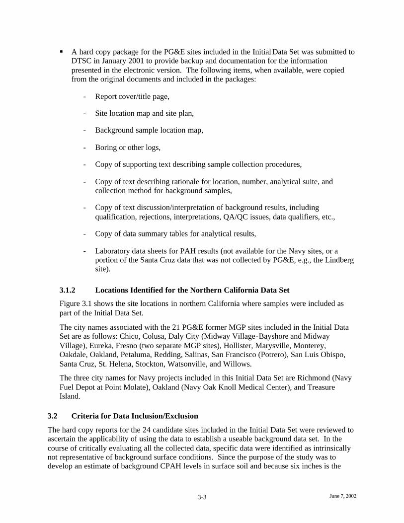
§ A hard copy package for the PG&E sites included in the Initial Data Set was submitted to DTSC in January 2001 to provide backup and documentation for the information presented in the electronic version. The following items, when available, were copied from the original documents and included in the packages:

- Report cover/title page,

- Site location map and site plan,

- Background sample location map,

- Boring or other logs,

- Copy of supporting text describing sample collection procedures,

- Copy of text describing rationale for location, number, analytical suite, and collection method for background samples,

- Copy of text discussion/interpretation of background results, including qualification, rejections, interpretations, QA/QC issues, data qualifiers, etc.,

- Copy of data summary tables for analytical results,

- Laboratory data sheets for PAH results (not available for the Navy sites, or a portion of the Santa Cruz data that was not collected by PG&E, e.g., the Lindberg site).

3.1.2 Locations Identified for the Northern California Data Set

Figure 3.1 shows the site locations in northern California where samples were included as part of the Initial Data Set.

The city names associated with the 21 PG&E former MGP sites included in the Initial Data Set are as follows: Chico, Colusa, Daly City (Midway Village-Bayshore and Midway Village), Eureka, Fresno (two separate MGP sites), Hollister, Marysville, Monterey, Oakdale, Oakland, Petaluma, Redding, Salinas, San Francisco (Potrero), San Luis Obispo, Santa Cruz, St. Helena, Stockton, Watsonville, and Willows.

The three city names for Navy projects included in this Initial Data Set are Richmond (Navy Fuel Depot at Point Molate), Oakland (Navy Oak Knoll Medical Center), and Treasure Island.

3.2 Criteria for Data Inclusion/Exclusion

The hard copy reports for the 24 candidate sites included in the Initial Data Set were reviewed to ascertain the applicability of using the data to establish a useable background data set. In the course of critically evaluating all the collected data, specific data were identified as intrinsically not representative of background surface conditions. Since the purpose of the study was to develop an estimate of background CPAH levels in surface soil and because six inches is the

June 7, 2002 3-4

most common definition of surface soil used in risk assessment, soil samples to a depth of 6 inches were considered appropriate for the background data set. Soil samples collected at depths greater than 6 inches were excluded from the background data set. Samples reported as not detected for all carcinogenic PAHs, with elevated detection limits (greater than 0.02 mg/kg) for one or more of the carcinogenic PAHs were also excluded from the data set due to the potential for such samples to bias the data set. Additionally, we excluded all duplicate samples and re-samples from the data set. Text, maps, and interpretation of results presented in the reports indicated that some samples designated to represent background, became suspect for that purpose either due to visual observations during sampling or analytical laboratory results. Accordingly, if a sample initially designated as background was indicated in the report as suspect for some reason, it was excluded from the Initial Data Set.

In summary, the following exclusion criteria were identified and applied to the Initial Data Set to eliminate from further consideration those samples that did not represent background conditions for PAHs. Samples to be excluded from the data set consisted of the following general categories (The codes mentioned below refer to entries in the electronic data base noting the basis for excluding each sample.):

§ Samples collected at depths of greater than six inches; (Code 1)

§ Samples reported as not detected for all CPAHs with elevated detection limits for one or more of the carcinogenic PAHs (i.e., greater than 0.02 mg/kg) (Code 2);

§ Duplicate samples or re-samples (Code 3); and

§ Samples that were identified as suspected of not representing background conditions (e.g., due to the potential presence of lampblack) in the original or subsequent site investigation reports; (Code 4)

This evaluation process resulted in the exclusion of 120 samples, leaving 156 samples for the Interim Data Set. Table 3.1 summarizes the samples excluded using this process. For Code 1, 35 samples were excluded from various sites. For Code 2, 66 samples were excluded from various sites. For Code 3, 11 samples were excluded for various sites. For Code 4, 8 samples were excluded from various sites. At this point in the evaluation, there was only one sample remaining for one of the Fresno sites and two samples remaining for the other Fresno site. The data from the two Fresno sites were combined and are used to represent background conditions in the Fresno area, which is counted as one site in the remaining sections of this report. As indicated in Table 3.1, the entire background data sets from two Navy Sites, Point Molate and Treasure Island, were excluded based on the fact that all samples were collected from depths of greater than six inches below ground surface. Thus, the Interim Data Set was composed of 155 samples from 20 different former MGP sites and one sample from the Navy Oak Knoll Medical Center, for a total of 156 samples.

4-1 June 7, 2002

4.0 PHASE 2: EVALUATION OF INTERIM DATA SET AND DEVELOPMENT OF THE FINAL DATA SET

This section describes the process by which the Interim Data Set of 156 samples was characterized and then further refined to generate the Final Data Set of 86 samples. Section 4.1 presents an evaluation of the Interim Data Set using statistical and graphical analyses. This evaluation includes comparisons among categories to investigate the homogeneity of the data set. Because consistency with a common distribution supports the hypothesis that the data set represents a single population, tests for normality and log-normality are included. Following these analyses, two of the sites (Redding and Midway Village) were determined to be over-represented in the Interim Data Set, with many more data points than any of the other sites. A method for addressing the potential bias int roduced by the over-representation of these two sites was developed in consultation with DTSC and is described in Section 4.2. Application of this method reduced the number of background samples to 88. As explained in Section 4.3, visual examination of the data across all sites resulted in the identification of two potential outliers. Subsequent investigation and further review of the two potential outliers resulted in the removal of these two samples from the data set, leaving a total of 86 background samples collected from 21 different sites. These samples are included in the Final Data Set.

One of the issues raised during evaluation of the Interim Data Set was the method used to develop B(a)P equivalent concentration values for samples in which some of the CPAHs were reported as “ND” or “non-detect.” The B(a)P equivalent concentrations in the Interim Data Set were calculated using ½ the detection limit to represent each non-detect. When detection limits are elevated, this practice is likely to result in overestimation of the actual B(a)P equivalent concentrations. As discussed in Section 4.4, a less biased method of assigning B(a)P equivalent concentrations to samples with one or more non-detect results was developed and applied to the 86 background samples in the Final Data Set. The evaluation and characterization of the Final Data Set is discussed in Section 5.0.

4.1 Evaluation of the Interim Data Set

As previously discussed, the purpose of this study was to develop a data set of CPAH surface soil concentrations that can be used to support background-based site investigation and remediation decisions. In determining whether the data set can be used for such purposes, one of the questions that must be addressed is whether the data set represents a single population. If there are differences among categories defined by geography, or if the data are not consistent with a common distribution, the data set may be better characterized as a mixture of data from distinct sub-populations.

The Interim Data Set includes 156 background samples collected at 21 sites in northern California. (The three data points in the interim data set collected from Fresno 1 and Fresno 2 sites are combined and discussed as a single Fresno site). Summary statistics for the B(a)P equivalent concentrations and their logarithms are presented in Table 4.1. The statistics are calculated for each site as well as for the entire data set. The preponderance of data from two of the sites (52 samples from Midway Village and 28 samples from Redding) is notable, as is the large number of censored samples from the Midway Village site. Censored samples are those in

4-2 June 7, 2002

which none of the seven CPAHs was detected; the B(a)P equivalent concentrations assigned to these samples are based on reported detection limits, rather than measurements.

The graphical and statistical methods discussed in Section 2.2 were used to evaluate the Interim Data Set. The results of these evaluations are described in this section. Graphical evaluations were conducted in conjunction with statistical tests. Box and whisker plots, scatter plots, and nonparametric (Kruskal-Wallis and Mann-Whitney) tests were used to investigate the sources of variation within the data set. Probability plots and Shapiro-Wilk tests were used to examine the consistency of the data set with the normal and lognormal distributions. All of the hypothesis tests presented in this study were evaluated at the five percent (0.05) level of significance.

4.1.1 Comparisons Among Categories

The initial statistical analysis of the Interim Data Set focused on determining whether there are systematic differences in the background data collected from different sites or categories of sites. The 156 samples in the Interim Data Set were collected from 21 sites (as described above, data from two separate sites in Fresno were combined and counted as one site) in northern California. The ability of each of four categorical variables to explain the observed variability in the B(a)P equivalent concentrations was evaluated. These four variables are:

§ Site - the site at which the background sample was collected

§ Region - the climatic region of northern California in which the site is located (northern, central, or southern)

§ Coastal versus Inland– the proximity of the site to the ocean (coastal versus inland location)

§ Number of Detects – the number of CPAHs detected in the background sample.

Two other categorical variables, laboratory method and laboratory, were also considered. Analyses for these two factors are not presented in this report because these variables are strongly related to the Site variable and do not add significant information to the overall analysis.

The significance of the four categorical variables (Site, Region, Coastal, and Number of Detects) was investigated by visual inspection of the plotted data and nonparametric hypothesis tests. For each categorical variable, the null hypothesis was that the medians of the categories defined by the variable are equal. Box and Whisker plots and scatter plots were used to illustrate the variation within and between categories, and Kruskal-Wallis and Mann-Whitney tests were used to compare the medians. Nonparametric tests were used because the amount of data available in some categories was not sufficient to allow meaningful tests of the assumptions required for parametric tests.

The significance of the categorical variables is summarized in Table 4.2 and Figures 4.1 through 4.4. The results of the hypothesis tests indicate that there are significant differences in the median values among the categories defined by each of the four variables. Figure 4.1

4-3 June 7, 2002

illustrates the evaluation of the Site variable. As indicated in Figure 4.1, the median CPAH concentrations vary from site to site. This graphical observation of site-to-site variability is supported by the results of the Kruskal-Wallis test (presented in Table 4.2), which indicate that there are significant differences among the median B(a)P equivalent concentrations in background samples collected at the different sites. The highest B(a)P equivalent concentrations are associated with the Stockton and Potrero sites.

Figure 4.2 illustrates the test of medians among the regions, and indicates that the median B(a)P concentration is lower in the Central region than in the Northern and Southern regions. As shown in Table 4.3, Midway Village is in the Central region. The large number of non-detects associated with the Midway Village site may be the primary reason that the median for the Central region is lower. The Central region also includes the Stockton and Potrero sites, which (as shown in Figure 4.1) have the highest B(a)P equivalent concentrations. These high values have much less influence on the median than they do on the mean value, so the mean concent rations for the three regions may not be significantly different even though the medians are.

Figure 4.3 illustrates the comparison between the categories based on proximity to the ocean (coastal versus inland location). The sites included in each category are listed in Table 4.4 . Midway Village is a coastal site, and the median value for the coastal sites is lower than the median value for the inland sites. Potrero is in the coastal category, while Stockton is in the inland category. These observations suggest that the large number of non-detects from Midway Village may be the primary cause of the difference in medians, and that the difference in means may not be significant.

Figure 4.4 is a scatter plot that illustrates the relationship between the number of CPAHs detected in a sample and its B(a)P equivalent concentration. As expected, the B(a)P equivalent concentration generally increases with the number of CPAHs detected in the sample. The Kruskal-Wallis test of this relationship presented in Table 4.2 demonstrates that the differences among the medians of the categories defined by the number of CPAHs detected are statistically significant. Figure 4.4 also shows a cluster of samples in which no CPAHs were detected that have low B(a)P equivalent concentrations. The B(a)P equivalent concentrations assigned to many of these samples are tied (i.e., the same CPAH value is assigned to more than one sample); as explained in section 2.2.1.2, a random offset is used to avoid having these data plot as a single point. This cluster includes many samples collected at the Midway Village site. Overall, Figure 4.4 and the related hypothesis test confirm the significance of the relationship between the B(a)P equivalent concentration and the number of CPAHs detected in a sample. Because this relationship is not relevant to the significance of the geographic variables, it was not investigated further in this study.

In summary, Table 4.2 and Figures 4.1 through 4.4 indicate that there are significant differences in the medians of the categories defined by each variable. The comparisons based on the Region and Coastal variables suggest that the median values are related to geographic location. These results, however, appear to be due, in large measure, to the inclusion of many Midway Village samples in which all of the CPAHs were reported as non-detects.

4-4 June 7, 2002

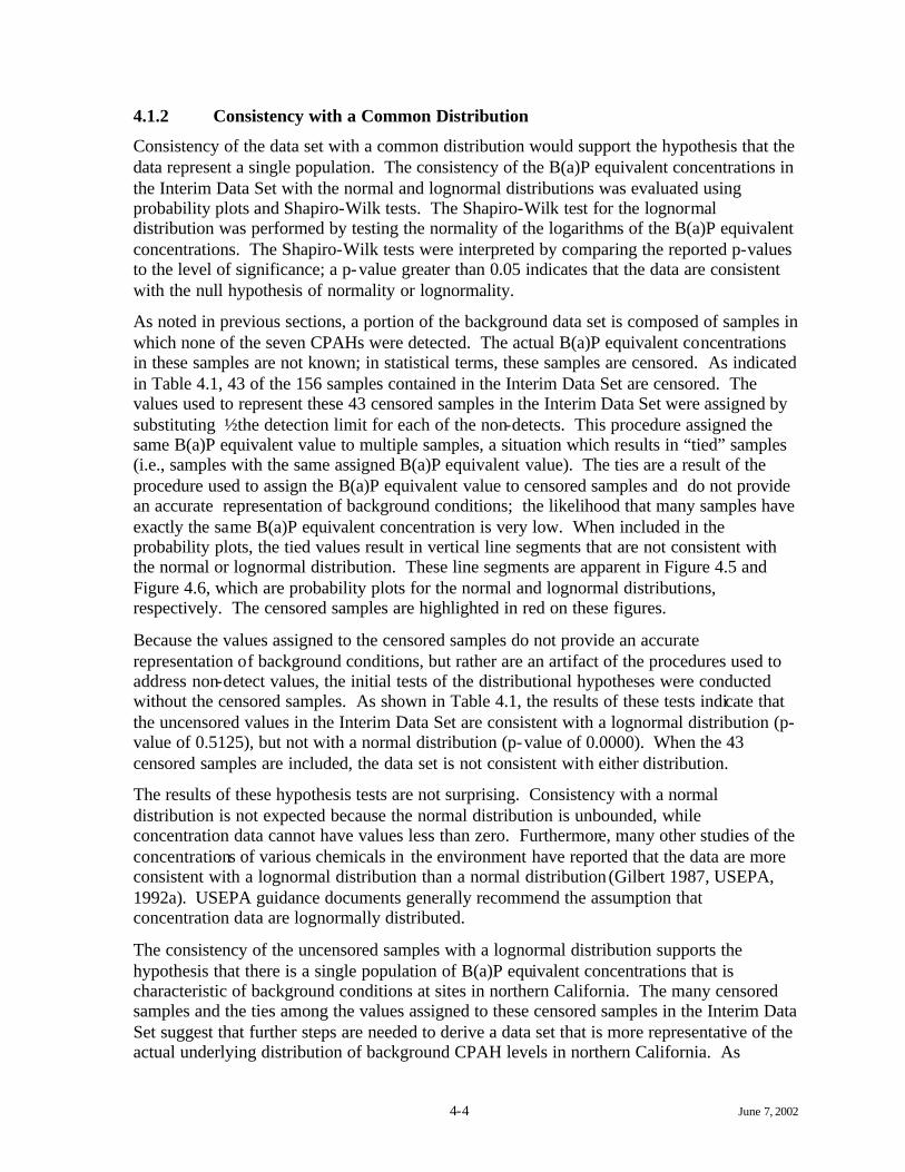
4.1.2 Consistency with a Common Distribution

Consistency of the data set with a common distribution would support the hypothesis that the data represent a single population. The consistency of the B(a)P equivalent concentrations in the Interim Data Set with the normal and lognormal distributions was evaluated using probability plots and Shapiro-Wilk tests. The Shapiro-Wilk test for the lognormal distribution was performed by testing the normality of the logarithms of the B(a)P equivalent concentrations. The Shapiro-Wilk tests were interpreted by comparing the reported p-values to the level of significance; a p-value greater than 0.05 indicates that the data are consistent with the null hypothesis of normality or lognormality.

As noted in previous sections, a portion of the background data set is composed of samples in which none of the seven CPAHs were detected. The actual B(a)P equivalent concentrations in these samples are not known; in statistical terms, these samples are censored. As indicated in Table 4.1, 43 of the 156 samples contained in the Interim Data Set are censored. The values used to represent these 43 censored samples in the Interim Data Set were assigned by substituting ½ the detection limit for each of the non-detects. This procedure assigned the same B(a)P equivalent value to multiple samples, a situation which results in “tied” samples (i.e., samples with the same assigned B(a)P equivalent value). The ties are a result of the procedure used to assign the B(a)P equivalent value to censored samples and do not provide an accurate representation of background conditions; the likelihood that many samples have exactly the same B(a)P equivalent concentration is very low. When included in the probability plots, the tied values result in vertical line segments that are not consistent with the normal or lognormal distribution. These line segments are apparent in Figure 4.5 and Figure 4.6, which are probability plots for the normal and lognormal distributions, respectively. The censored samples are highlighted in red on these figures.

Because the values assigned to the censored samples do not provide an accurate representation of background conditions, but rather are an artifact of the procedures used to address non-detect values, the initial tests of the distributional hypotheses were conducted without the censored samples. As shown in Table 4.1, the results of these tests indicate that the uncensored values in the Interim Data Set are consistent with a lognormal distribution (p-value of 0.5125), but not with a normal distribution (p-value of 0.0000). When the 43 censored samples are included, the data set is not consistent with either distribution.

The results of these hypothesis tests are not surprising. Consistency with a normal distribution is not expected because the normal distribution is unbounded, while concentration data cannot have values less than zero. Furthermore, many other studies of the concentrations of various chemicals in the environment have reported that the data are more consistent with a lognormal distribution than a normal distribution (Gilbert 1987, USEPA, 1992a). USEPA guidance documents generally recommend the assumption that concentration data are lognormally distributed.

The consistency of the uncensored samples with a lognormal distribution supports the hypothesis that there is a single population of B(a)P equivalent concentrations that is characteristic of background conditions at sites in northern California. The many censored samples and the ties among the values assigned to these censored samples in the Interim Data Set suggest that further steps are needed to derive a data set that is more representative of the actual underlying distribution of background CPAH levels in northern California. As

4-5 June 7, 2002

described below, these steps include balancing the data set, eliminating outliers, and re-calculating the B(a)P equivalent concentrations assigned to samples in which some of the CPAHs were not detected.

4.2 Reduction of Data Points Associated with Midway Village and Redding Sites

As discussed in Section 3, application of the four exclusion criteria produced an Interim Data Set that includes 156 samples from 21 sites. This data set includes 52 samples from Midway Village and 28 samples from Redding, with an average of only four samples from each of the other sites. After discussions with the DTSC, it was decided that the background data set should be balanced to avoid over-representation of any particular site or local area. Therefore, the numbers of samples from the Midway Village and Redding sites were reduced so all sites would be evenly represented in the background data set. To reduce the number of samples, the data from each of the two over-represented sites (Midway Village and Redding) were ranked and one sample was randomly selected from each 1/6 quantile, yielding six samples from each site for inclusion in the background data set. As a result of this process, a total of 68 samples were removed from the data set (46 samples from Midway Village and 22 samples from Redding) leaving a total of 88 samples.

4.3 Identification of Outliers and Further Reduction of the Interim Data Set

Further review of the Interim Data Set was performed to identify possible outliers. Visual inspection of the box and whisker plot in Figure 4.1 identified two sites with elevated B(a)P equivalent concentrations, Stockton and Potrero. The data associated with these sites were re-examined for their ability to represent background conditions. Visits to these two sites revealed that Stockton sample SS-10 (with a B(a)P equivalent concentration of 11.8 mg/kg) and Potrero sample BSS-POT-4 (with a B(a)P equivalent concentration of 6.3 mg/kg) may not represent background concentrations. An investigation of the sampling locations associated with these two samples indicated that they may have been collected from areas where the PAHs in soil could have come from specific industrial sources. For this reason, a conservative approach was taken and these two samples were removed from the data set, leaving a total of 86 samples. Table 4.5 summarizes the samples excluded through the reduction of data points associated with the Midway Village and Redding sites and the removal of outliers.

4.4 Treatment of Non-Detects and Elevated Detection Limits

The evaluation of the Interim Data Set was complicated by the presence of many samples in which no CPAHs were detected and by the fact that the same B(a)P equivalent value was assigned to many of these censored samples. As previously discussed, the tied values, which do not accurately represent background conditions, distort the hypothesis tests. The results of these tests should not be determined by the values assigned to censored samples simply by substituting ½ the detection limit for each non-detect because ½ the detection limit is not likely to be an accurate estimate of actual concentration. The problems caused by the censored samples were addressed in part by balancing the data set to eliminate having a disproportionate number of samples for any one site. Of the 68 samples from the Midway Village and Redding sites that were removed, 30 were censored samples in which no CPAHs were detected. Only 13 of the 86 samples (15 percent) selected for inclusion in the Final Data Set were censored.

4-6 June 7, 2002

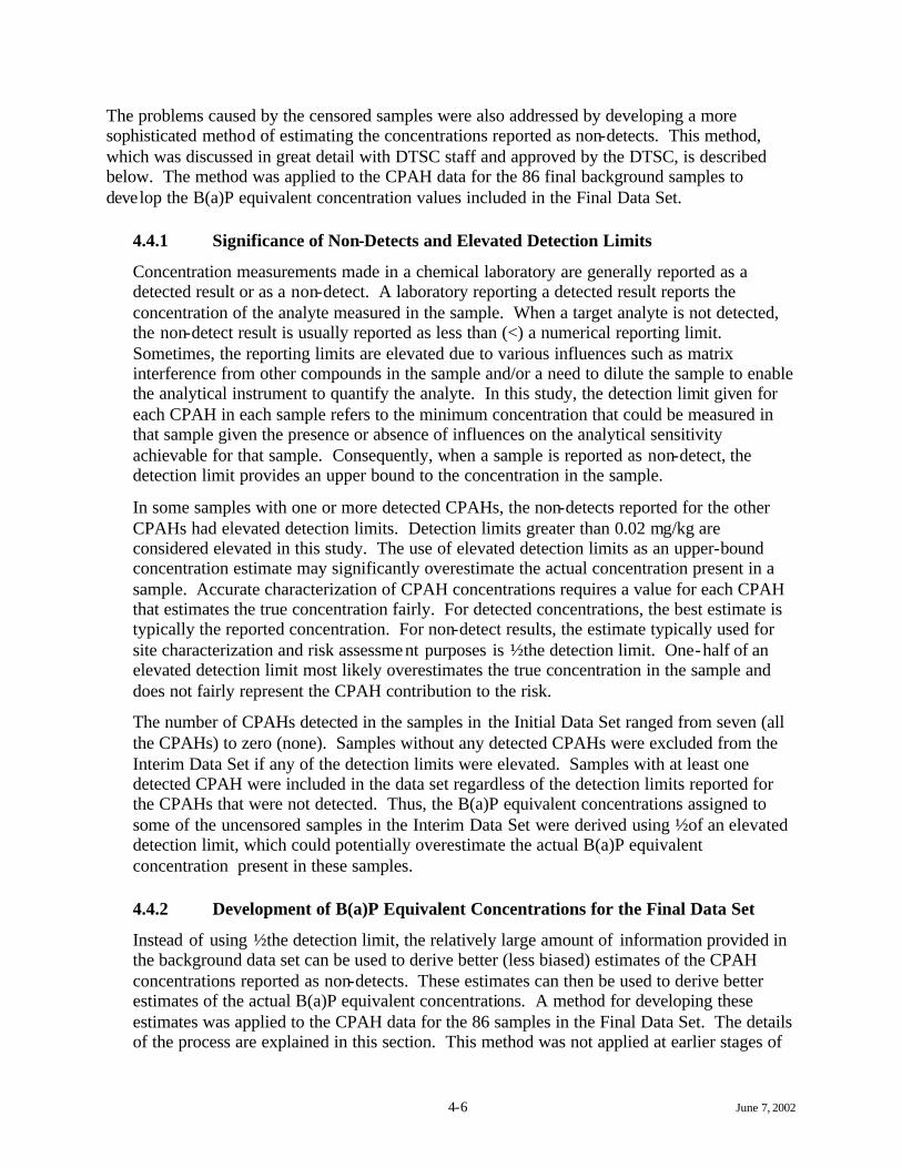
The problems caused by the censored samples were also addressed by developing a more sophisticated method of estimating the concentrations reported as non-detects. This method, which was discussed in great detail with DTSC staff and approved by the DTSC, is described below. The method was applied to the CPAH data for the 86 final background samples to develop the B(a)P equivalent concentration values included in the Final Data Set.

4.4.1 Significance of Non-Detects and Elevated Detection Limits

Concentration measurements made in a chemical laboratory are generally reported as a detected result or as a non-detect. A laboratory reporting a detected result reports the concentration of the analyte measured in the sample. When a target analyte is not detected, the non-detect result is usually reported as less than (<) a numerical reporting limit. Sometimes, the reporting limits are elevated due to various influences such as matrix interference from other compounds in the sample and/or a need to dilute the sample to enable the analytical instrument to quantify the analyte. In this study, the detection limit given for each CPAH in each sample refers to the minimum concentration that could be measured in that sample given the presence or absence of influences on the analytical sensitivity achievable for that sample. Consequently, when a sample is reported as non-detect, the detection limit provides an upper bound to the concentration in the sample.

In some samples with one or more detected CPAHs, the non-detects reported for the other CPAHs had elevated detection limits. Detection limits greater than 0.02 mg/kg are considered elevated in this study. The use of elevated detection limits as an upper-bound concentration estimate may significantly overestimate the actual concentration present in a sample. Accurate characterization of CPAH concentrations requires a value for each CPAH that estimates the true concentration fairly. For detected concentrations, the best estimate is typically the reported concentration. For non-detect results, the estimate typically used for site characterization and risk assessment purposes is ½ the detection limit. One-half of an elevated detection limit most likely overestimates the true concentration in the sample and does not fairly represent the CPAH contribution to the risk.

The number of CPAHs detected in the samples in the Initial Data Set ranged from seven (all the CPAHs) to zero (none). Samples without any detected CPAHs were excluded from the Interim Data Set if any of the detection limits were elevated. Samples with at least one detected CPAH were included in the data set regardless of the detection limits reported for the CPAHs that were not detected. Thus, the B(a)P equivalent concentrations assigned to some of the uncensored samples in the Interim Data Set were derived using ½ of an elevated detection limit, which could potentially overestimate the actual B(a)P equivalent concentration present in these samples.

4.4.2 Development of B(a)P Equivalent Concentrations for the Final Data Set

Instead of using ½ the detection limit, the relatively large amount of information provided in the background data set can be used to derive better (less biased) estimates of the CPAH concentrations reported as non-detects. These estimates can then be used to derive better estimates of the actual B(a)P equivalent concentrations. A method for developing these estimates was applied to the CPAH data for the 86 samples in the Final Data Set. The details of the process are explained in this section. This method was not applied at earlier stages of

4-7 June 7, 2002

the analysis because it is time-consuming; removing a single sample from the data set may require re-calculation of the values assigned to many of the remaining samples.

The detection limits reported for each CPAH varied from one sample to another, both within and between sites (In the Final Data Set, detection limits ranged from 0.00038 mg/kg to 2.5 mg/kg). Some of the elevated detection limits were higher than detected concentrations in other samples. For example, one sample may have benzo(a)pyrene reported as not detected at a detection limit of 70 µg/kg, while another sample may have a detection of the same CPAH reported at 50 µg/kg. The detected concentrations that are lower than the elevated detection limits for a CPAH provide information that can be used to estimate the concentration of the CPAH in the samples with elevated detection limits. For each CPAH, a representative concentration value for each non-detect reported with an elevated detection limit was calculated by averaging all of the representative values below the elevated detection limit. This process is applied starting with the lowest of the elevated detection limits and working upward because a representative value must be assigned to all samples with lower elevated detection limits before one can be assigned to a sample with higher elevated detection limits. The following steps outline the process for assigning the representative values for each CPAH:

1. The samples, detected and non-detects, were rank ordered from highest to lowest, using the detection limit for the non-detects and the reported concentration for the detected.

2. Samples in which the CPAH was detected were assigned a representative value equal to the reported concentration.

3. Samples with non-detect results and a detection limit of 0.02 mg/kg or lower were assigned a representative value equal to ½ the detection limit.

4. The non-detect result with the lowest of the elevated detection limits (i.e., the lowest of the detection limits that were greater than 0.02 mg/kg) was identified.

5. The representative values from the samples lower in the rank order than the sample identified in step 4 were averaged.

6. The average was assigned as the representative value of the sample identified in step 4.

7. The non-detect result with the next lowest elevated detection limit was identified.

8. The representative values from the samples lower in the rank order than the sample identified in step 7 were averaged.

9. The average was assigned as the representative value of the sample identified in step 7.

10. Steps 7 through 9 were repeated until all samples with elevated non-detects were assigned a representative value.

The representative values assigned by this process for each CPAH are dependent on the other values included in the data set. Thus, adding or removing samples from the data set may change the assigned values for many samples. After representative values for each CPAH

4-8 June 7, 2002

were assigned to each sample, the B(a)P equivalent concentration was calculated using the Cal/EPA toxicity equivalent factors provided in the data set.

5-1 June 7, 2002

5.0 PHASE 3: EVALUATION OF THE FINAL DATA SET

The final data set produced by the process described in the preceding sections contains 86 samples of surface soil from background locations at 21 sites in northern California. Summary statistics for the B(a)P equivalent concentrations calculated for these samples are provided in Table 5.1. The number of samples per site ranges from 1 to 9 with an average of 4. The data set includes 13 censored samples in which no CPAHs were detected. These 13 are distributed as follows: 4 at Colusa, 3 at Midway Village, 1 at Redding, 1 at Salinas, and 4 at Santa Cruz.

The graphical and statistical methods applied to the Interim Data Set in Section 4.1 were used to evaluate the Final Data Set. The results of these evaluations are described in this section. All of the hypothesis tests presented in this study were evaluated at the five percent (0.05) level of significance.

5.1 Comparisons Among Categories

The ability of each of three categorical variables to explain the observed variability in the B(a)P equivalent concentrations in the Final Data Set was evaluated. These three variables (Site, Region, and Coastal vs. Inland) are defined in Section 4.1.1, and the assignment of sites to the Region and Coastal categories is as shown in Tables 4.3 and 4.4, respectively.

Evaluation of the data for similarities and differences among the sites, regions, and coastal categories are shown in box and whisker plots (Figures 5.1 through 5.3). The results of the corresponding nonparametric hypothesis tests are presented in Table 5.2. The range of the B(a)P equivalent concentrations in the final 86-sample data set is smaller than that in the larger data sets evaluated earlier, but variability among the sites is still evident. Figure 5.1 and the p-value of the first Kruskal-Wallis test (0.001 in Table 5.2) both indicate that there are significant differences among the median concentrations of the various sites. On the other hand, the comparison between the regional categories (Figure 5.2) shows a high degree of similarity. The Kruskal-Wallis test for this comparison (Table 5.2) has a p-value of 0.98, which indicates that there are no significant differences among the medians for the three regions. Similarly, the medians of the categories defined by proximity to the ocean (coastal and non-coastal) are not significantly different. This comparison is shown in Figure 5.3 and supported by the Mann-Whitney test, which has a p-value of 0.632.

Taken all together, these comparisons indicate that while there may be significant differences between the medians for some sites, these differences are not related to the locations of the sites within northern California. There are no consistent differences between sites in the three geographic regions (north, central, and south) or between the coastal and non-coastal categories. The observed site-to-site variability does not appear to be related to any of the identified variables and is likely random. These results indicate that the Final Data Set provides a reasonable characterization of the background levels of CPAHs in surface soils in all parts of northern California.

5-2 June 7, 2002

5.2 Consistency with a Common Distribution

The distributions of the B(a)P equivalent concentrations in the Final Data Set and their logarithms are illustrated as probability plots in Figure 5.4 and Figure 5.5, respectively. The Final Data Set includes 13 samples in which none of the CPAHs were detected. These 13 censored samples are highlighted red in the probability plots. The process used to handle the non-detects in calculating the B(a)P equivalent value (described in section 4.4) assigned the same B(a)P equivalent value to many of these 13 samples. The tied values among these 13 samples cause vertical lines in the probability plots that are not consistent with the normal or lognormal distribution. The tied B(a)P equivalent concentrations assigned to the censored samples do not provide an accurate representation of background conditions and are merely an artifact of the process used to assign values to non-detects.

The consistency of the Final Data Set with a common distribution should be evaluated using B(a)P equivalent concentrations that are representative of actual background conditions. Therefore, the consistency of the Final Data Set with a lognormal distribution was evaluated by performing the Shapiro-Wilk test of normality on the logarithms of the 73 uncensored samples. As shown in Table 5.3, this test provides a p-value of 0.8091, which indicates that the B(a)P equivalent concentrations for the uncensored samples are quite consistent with a lognormal distribution. The distribution of the logarithms of the B(a)P equivalents associated with the 73 uncensored samples is illustrated as a probability plot in Figure 5.6. The p-value obtained when the logarithms of the censored samples were included was only 0.0078. Comparison of these p-values demonstrates that the 73 uncensored values are consistent with the log-normal distribution, but that the full set of 86 B(a)P equivalent concentrations is not consistent with a lognormal distribution due to the ties in the values assigned to the 13 censored samples.

The Final Data Set fails the Shapiro-Wilk test for normality regardless of whether the censored samples are included. This result is expected for the reasons explained in section 4.1.2. The consistency of the uncensored samples in the Final Data Set with the lognormal distribution provides strong support for the hypothesis that these background data represent a single population.

5.3 Development of the Smoothed Data Set

The B(a)P equivalent concentrations assigned to the censored samples in the Final Data Set may affect the values of descriptive statistics such as the mean, standard deviation, and upper confidence limit. To represent the background population accurately, these statistics should be calculated using values that are representative of background conditions and consistent with the lognormal distribution defined by the uncensored samples. Therefore, a more realistic set of B(a)P equivalent concentrations was developed to represent the 13 censored samples in calculating descriptive statistics.

A number of methods of compensating for censored data have been described in the scientific literature, but most of these methods were developed for situations in which all values below a single detection limit are censored. Such methods are described and recommended in USEPA guidance documents such as Guidance for Data Quality Assessment (USEPA 2000) and Statistical Analysis of Ground-Water Monitoring Data at RCRA Facilities – Addendum to Interim Final Guidance (USEPA 1992a). The characteristics of the censored samples in the Final Data Set are not consistent with these methods; although the initial B(a)P equivalent

5-3 June 7, 2002

concentrations assigned to the censored samples are all in the lower end of the distribution, these values are interspersed with the measured (uncensored) concentrations. This situation, in which different samples are censored at different detection limits, is referred to in the literature as multiple censoring.

In this study, the 13 censored samples were addressed by a robust method based on probability plotting. The basic method is described in section 13.1.3 of Helsel and Hirsch (1992). It involves plotting the uncensored data on probability paper, fitting a line, and using the line to estimate the values for the censored samples. This procedure uses all of the data obtained from the uncensored samples to estimate new, more realistic values for the censored samples. As applied in this study, the new values for the censored samples were estimated using an exponential model calibrated in the B(a)P equivalent space, rather than by linear regression in the log-transformed space. Calibration in the B(a)P space is necessary to avoid biased estimates.

Application of this method results in a smoothed data set that includes 86 B(a)P equivalent values that are consistent with the lognormal distribution defined by the uncensored samples, and with the number and ranks of the B(a)P equivalent concentrations initially assigned to the censored samples. The probability plot of the logarithms of the B(a)P equivalent concentrations associated with the smoothed data set is shown in Figure 5.7. This figure demonstrates that the vertical line segments that represented the tied values initially assigned to the censored samples have been smoothed out. The Shapiro-Wilk test of normality performed on the logarithms of the smoothed data set (shown in Table 5.3) resulted in a p-value of 0.1575, which indicates that the smoothed data set (86 values) is consistent with the lognormal distribution. As noted previously, this consistency supports the hypothesis that the background data represent a single population.

Because the 13 B(a)P equivalent concentrations obtained by smoothing are more consistent with background conditions than the values that were originally assigned to the censored samples, the descriptive statistics of the Final Data Set should be calculated with the smoothed values. As presented in Table 5.3, the arithmetic mean and standard deviation of the smoothed data set are 0.2143 and 0.4161 mg/kg, respectively. These statistics are essentially equivalent to the mean and standard deviation of the 86 B(a)P equivalent concentrations in the Final Data Set before smoothing, which are 0.2137 and 0.4164 mg/kg. Thus, the smoothing procedure had little effect on the mean and standard deviation. In contrast, the mean and standard deviation calculated for the 73 uncensored samples only are 0.2507 and 0.4422 mg/kg, respectively (see Table 5.3). The fact that these statistics for the uncensored samples only are higher than those obtained when the censored samples are accounted for demonstrates the importance of accounting for the censored samples when characterizing the population of background concentration values. These results indicate that it is important to account for the censored samples, and that smoothing had little effect on the descriptive statistics.

Although smoothing had very little effect on the mean and standard deviation, the effect on statistics used to represent the upper tail of the distribution is much more significant. The upper-tail statistics presented in Table 5.3 include the 95th percentile upper confidence limit (UCL) on the population mean; the upper tolerance limit (UTL) for 95 percent confidence and 95 percent coverage; and the 95th percentile of the distribution. Use of the 13 B(a)P equivalent values obtained for the censored samples by smoothing resulted in a reduction of about 10 percent in both the UCL and the UTL in comparison to the values calculated for the Final Data Set Before Smoothing. The 95th percentile was not affected because all of the censored samples are in the

5-4 June 7, 2002

lower end of the distribution. The reductions in the UCL and UTL demonstrate the importance of using the values obtained by smoothing (which are consistent with the distribution of background values defined by the uncensored samples) rather than the tied values previously assigned to the censored samples when calculating descriptive statistics.

Smoothing of the Final Data Set in this fashion does not affect the comparisons among categories presented in Section 5.1, which were performed prior to smoothing. The B(a)P equivalent concentrations originally assigned to 11 of the 13 censored samples were tied; the 11 tied samples included a group of 9 with an assigned value of 0.005475 mg/kg and a pair of two with an assigned value of 0.007665 mg/kg. As a result of these ties, 11 of the 13 smoothed values cannot be associated with a specific censored sample. Consider the two censored samples that were tied at an assigned value of 0.007665 mg/kg. Smoothing produced two new values (0.017612 and 0.016443 mg/kg), to represent these two tied samples; but there is no way of deciding which of the two new values should be assigned to which of the two censored samples. In the case of the two tied samples, this is not important because both were collected in the same study (Colusa 2000) at the same site. The 9 tied samples, however,were collected at three different sites; assigning the 9 new values (all different) to these 9 censored samples in an arbitrary way would affect the summary statistics for each site and could alter the results of site-to-site comparisons. Therefore, the censored samples that were originally tied cannot be represented by the smoothed values when evaluating the differences among categories defined by site, region, and proximity to ocean.

6-1 June 7, 2002

6.0 SUMMARY AND CONCLUSIONS

The data set of background CPAH concentrations generated by the process described in the preceding sections was developed to support site management decisions involving a comparison of site data to background CPAH data. The data set was developed to represent CPAH levels in surface soil in northern California. In this context, the utility of the data set is determined in part by its statistical characteristics. To make best use of the data set, users of the background data set should be familiar with the characteristics of the data set discussed in Section 5.0.

This Final Data Set contains values for 86 samples of surface soil collected from background locations at 21 sites across northern California. Each sample is represented in the data set by a single value, the B(a)P equivalent concentration. The B(a)P equivalent concentrations in the Final Data Set were calculated using toxicity equivalent factors proposed by the California Environmental Protection Agency in conjunction with the measured concentration of each CPAH. Non-detects for the individual CPAHs were handled by the procedure described in Section 4.4.

A smoothing procedure was used to compensate for the impact of the censored samples on the descriptive statistics used to characterize the Final Data Set. The potential impact of censored samples on these statistics is described in USEPA guidance documents (USEPA 2000). Smoothing of the data set produced 86 B(a)P equivalent concentrations that are consistent with the lognormal distribution defined by the uncensored samples and with the number and relative ranks of the B(a)P equivalent concentrations initially assigned to the censored samples.

The process of selecting the Final Data Set included the critical evaluation of the data to identify samples considered representative of background. While statistical methods were used to identify data points that appeared anomalous, judgment regarding site-specific information was necessarily an element in determining whether a sample represented background conditions (i.e., whether it was a valid background sample). The need to include judgment in the selection of data to be included in the Final Data Set is in part related to the fact that PAHs found in the surface soil come from multiple sources including urban fallout and natural sources, as well as specific industrial and domestic sources. Debate continues regarding the practical definition of background and, in particular, the degree to which PAHs from specific industrial and domestic sources should be considered background PAHs. The debate is complicated by the fact that it is not usually possible to distinguish the specific sources of PAHs in background samples. As a practical measure in this project, however, we have eliminated samples that appeared to represent observable contamination from specific industrial or domestic sources.

The Interim Data Set and the Final Data Set were both examined to determine whether dividing the data into categories based on geographic variables would provide a better representation of background levels of CPAH within northern California. The differences among the geographic categories were statistically significant in the Interim Data Set, but were not in the Final Data Set. Balancing the data set among the sites and eliminating two outliers and many of the censored samples resulted in a more homogeneous data set. The remaining variation is not related to the geographic variables, so the Final Data Set is considered to be representative of conditions across northern California. The results of the multiple graphical and statistical evaluations performed to characterize the data set lead us to conclude that the Final Data Set is

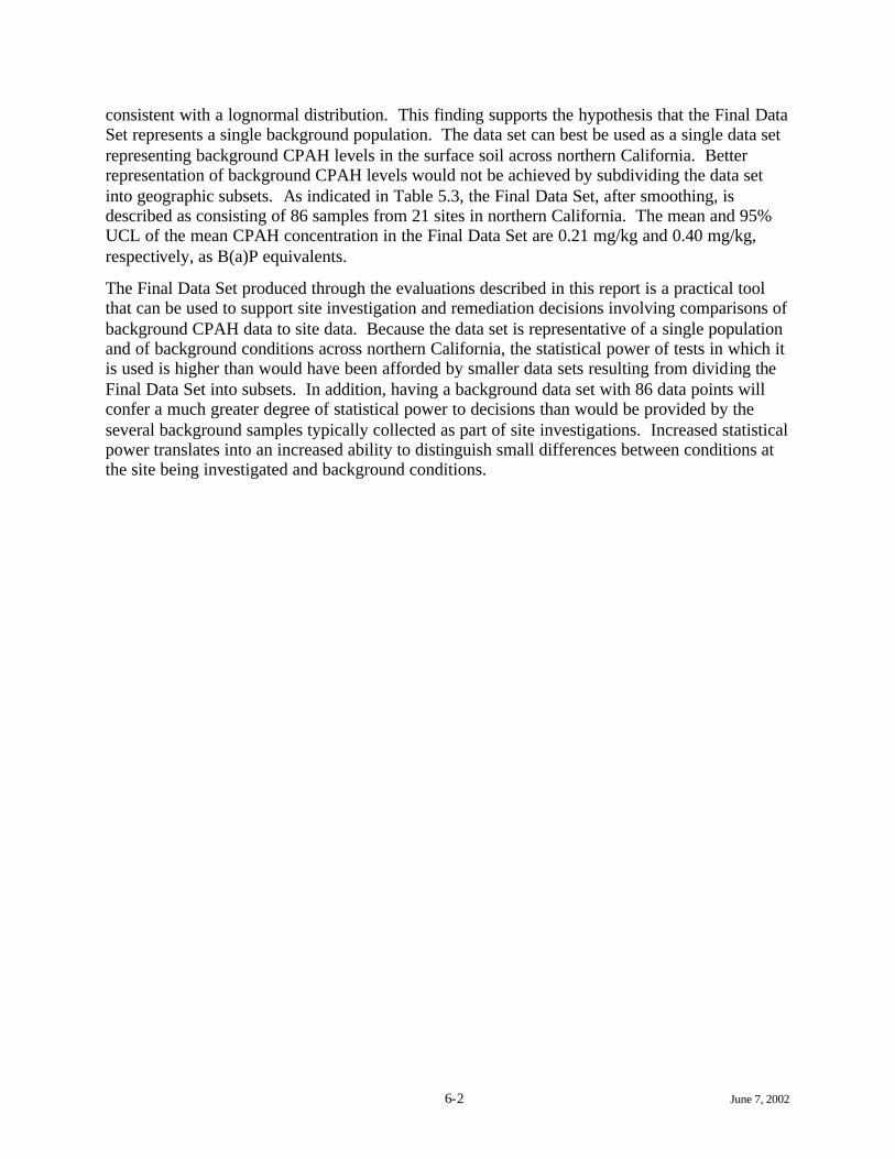
6-2 June 7, 2002

consistent with a lognormal distribution. This finding supports the hypothesis that the Final Data Set represents a single background population. The data set can best be used as a single data set representing background CPAH levels in the surface soil across northern California. Better representation of background CPAH levels would not be achieved by subdividing the data set into geographic subsets. As indicated in Table 5.3, the Final Data Set, after smoothing, is described as consisting of 86 samples from 21 sites in northern California. The mean and 95% UCL of the mean CPAH concentration in the Final Data Set are 0.21 mg/kg and 0.40 mg/kg, respectively, as B(a)P equivalents.

The Final Data Set produced through the evaluations described in this report is a practical tool that can be used to support site investigation and remediation decisions involving comparisons of background CPAH data to site data. Because the data set is representative of a single population and of background conditions across northern California, the statistical power of tests in which it is used is higher than would have been afforded by smaller data sets resulting from dividing the Final Data Set into subsets. In addition, having a background data set with 86 data points will confer a much greater degree of statistical power to decisions than would be provided by the several background samples typically collected as part of site investigations. Increased statistical power translates into an increased ability to distinguish small differences between conditions at the site being investigated and background conditions.

R-1 June 7, 2002

REFERENCES

Agency for Toxic Substances and Disease Regis try (ATSDR). 1999. ATSDR’s Toxicological Profiles on CD-ROM. CRC Press, LLC.

Gilbert, R.O. 1987. Statistical Methods for Environmental Pollution Monitoring. Van Nostrand Reinhold Company.

Helsel, D. R. and R. M. Hirsch. 1992b. Statistical Methods in Water Resources. Elsevier Science Publishers.

Cal/EPA 1994. Benzo(a)pyrene as a Toxic Air Contaminant. California Air Resources Board (CARB). July.

Jones, K.C., Stratford, J.A., Waterhouse, K.S., Furlong, E.T., Giger, W., Hites, R.A., Schaffner, C., and Johnson, A.E. 1989. Increases in the Polynuclear Aromatic Hydrocarbon Content of an Agricultural Soil over the Last Century: Environmental Science and Technology, Vol. 23, No. 1, pgs. 95 - 101.

Mazzera, D., Hayes, T., Lowenthal, D., and Zielinska, B. 1999. Quantification of polycyclic aromatics hydrocarbons in soil at McMurdo Station, Antarctica: The Science of the Total Environment, No. 229, pgs. 65 - 71.

USEPA 1992a. Statistical Analysis of Ground-Water Monitoring Data at RCRA Facilities – Addendum to Interim Final Guidance. Office of Solid Waste Management. February.

USEPA 1992b. Supplemental Guidance to RAGS: Calculating the Concentration Term. Office of Solid Waste and Emergency Response. May.

USEPA 2000. Guidance for Data Quality Assessment: Practical Methods for Data Analysis, EPA QA/G-9, EPA/600/R-96/084, July. 34, No. 19, pgs.4064 - 4070 - PG&E PAH.

USEPA 2002. Region IX Preliminary Remediation Goals (PRGs). Online Background Information Document.

Van Metre, P.C., Mahler, B.J., and Furlong, E.T. 2000. Urban sprawl leaves its PAH signature: Environmental Science and Technology, Vol. 34, No. 19, pgs. 4064 – 4070.

T-1 June 7, 2002

TABLES

SiteSample Identification Rationale

Exclusion Code

Pointe Molate All 16 samples All samples were collected from a depth of greater than 6 inches, thus not representing surface soil conditions

1

Santa Cruz LB-1 (2 cm and 1 foot composite)

Sample composite includes soil collected 1 foot below ground surface. Not representative of surface soils

1

Santa Cruz LB-1 (1 foot) Sample collected from a depth greater than 6 inches below ground surface (bgs). Not representative of surface soils

1

Santa Cruz LB-10 (2 cm and 1 foot composite)

Sample composite includes soil collected 1 foot below ground surface. Not representative of surface soils

1

Santa Cruz LB-10 (1 foot) Sample collected in a location under a former building 1

Santa Cruz LB-2 (2 cm and 1 foot composite)

Sample composite includes soil collected 1 foot below ground surface. Not representative of surface soils

1

Santa Cruz LB-2 (1 foot) Sample collected from a depth greater than 6 inches below ground surface (bgs). Not representative of surface soils

1

Santa Cruz LB-3 (2 cm and 1 foot composite)

Sample composite includes soil collected 1 foot below ground surface. Not representative of surface soils

1

Santa Cruz LB-3 (1 foot) Sample collected from a depth greater than 6 inches below ground surface (bgs). Not representative of surface soils

1

Santa Cruz LB-4 (2 cm and 1 foot composite)

Sample composite includes soil collected 1 foot below ground surface. Not representative of surface soils

1

Santa Cruz LB-4 (1 foot) Sample collected from a depth greater than 6 inches below ground surface (bgs). Not representative of surface soils

1

Santa Cruz LB-6 (2 cm and 1 foot composite)

Sample composite includes soil collected 1 foot below ground surface. Not representative of surface soils

1

Santa Cruz LB-6 (1 foot) Sample collected from a depth greater than 6 inches below ground surface (bgs). Not representative of surface soils

1

Santa Cruz LB-9 (2 cm and 1 foot composite)

Sample composite includes soil collected 1 foot below ground surface. Not representative of surface soils

1

Santa Cruz LB-9 (1foot) Sample collected from a depth greater than 6 inches below ground surface (bgs). Not representative of surface soils

1

Santa Cruz P-26-1 Sample composite includes soil collected 1 foot below ground surface. Not representative of surface soils

1

Santa Cruz P-26-10 Sample collected in a location under a former building and adjacent to a potential contaminant source

1

Santa Cruz P-26-2 Sample collected in a location under a former building 1

Santa Cruz P-26-3 Sample composite includes soil collected 1 foot below ground surface. Not representative of surface soils.

1

Santa Cruz P-26-4 Sample composite includes soil collected 1 foot below ground surface. Not representative of surface soils.

1

Eureka SS-EKA-15 All concentrations were non-detect, with elevated detection limits (i.e., greater than 0.02mg.kg) for one or more of the CPAHs.

2

Eureka SS-EKA-18 All concentrations were non-detect, with elevated detection limits (i.e., greater than 0.02mg.kg) for one or more of the CPAHs.

2

Eureka SS-EKA-19 All concentrations were non-detect, with elevated detection limits (i.e., greater than 0.02mg.kg) for one or more of the CPAHs.

2

Fresno-1 DSS-10 All concentrations were non-detect, with elevated detection limits (i.e., greater than 0.02mg.kg) for one or more of the CPAHs.

2

Fresno-1 DSS-9 All concentrations were non-detect, with elevated detection limits (i.e., greater than 0.02mg.kg) for one or more of the CPAHs.

2

Fresno-2 DSS-FRS2-11 All concentrations were non-detect, with elevated detection limits (i.e., greater than 0.02mg.kg) for one or more of the CPAHs.

2

Fresno-2 DSS-FRS2-7 All concentrations were non-detect, with elevated detection limits (i.e., greater than 0.02mg.kg) for one or more of the CPAHs.

2

Midway-Bayshore

BS-1 All concentrations were non-detect, with elevated detection limits (i.e., greater than 0.02mg.kg) for one or more of the CPAHs.

2

Table 3.1: Samples Proposed for Exclusion from Initial Data Set

1 of 3 June 7, 2002

SiteSample Identification Rationale

Exclusion Code

Table 3.1: Samples Proposed for Exclusion from Initial Data Set

Midway-Bayshore

BS-10 All concentrations were non-detect, with elevated detection limits (i.e., greater than 0.02mg.kg) for one or more of the CPAHs.

2

Midway-Bayshore

BS-12 All concentrations were non-detect, with elevated detection limits (i.e., greater than 0.02mg.kg) for one or more of the CPAHs.

2

Midway Village

32 various samples (see database)

All concentrations were non-detect, with elevated detection limits (i.e., greater than 0.02mg.kg) for one or more of the CPAHs.

2

Oakdale DSS-OKD-10 All concentrations were non-detect, with elevated detection limits (i.e., greater than 0.02mg.kg) for one or more of the CPAHs.

2

Petaluma SS-PET-12 All concentrations were non-detect, with elevated detection limits (i.e., greater than 0.02mg.kg) for one or more of the CPAHs.

2

Petaluma SS-PET-13 All concentrations were non-detect, with elevated detection limits (i.e., greater than 0.02mg.kg) for one or more of the CPAHs.

2

Petaluma SS-PET-14 All concentrations were non-detect, with elevated detection limits (i.e., greater than 0.02mg.kg) for one or more of the CPAHs.

2

Petaluma SS-PET-16 All concentrations were non-detect, with elevated detection limits (i.e., greater than 0.02mg.kg) for one or more of the CPAHs.

2

Petaluma SS-PET-17 All concentrations were non-detect, with elevated detection limits (i.e., greater than 0.02mg.kg) for one or more of the CPAHs.

2

Potrero BSS-POT-5 All concentrations were non-detect, with elevated detection limits (i.e., greater than 0.02mg.kg) for one or more of the CPAHs.

2

Redding SS-RED-3 All concentrations were non-detect, with elevated detection limits (i.e., greater than 0.02mg.kg) for one or more of the CPAHs.

2

Redding BG-1 All concentrations were non-detect, with elevated detection limits (i.e., greater than 0.02mg.kg) for one or more of the CPAHs.

2

Salinas DSS-SAL-10 All concentrations were non-detect, with elevated detection limits (i.e., greater than 0.02mg.kg) for one or more of the CPAHs.

2

Salinas DSS-SAL-6 All concentrations were non-detect, with elevated detection limits (i.e., greater than 0.02mg.kg) for one or more of the CPAHs.

2

Salinas DSS-SAL-8 All concentrations were non-detect, with elevated detection limits (i.e., greater than 0.02mg.kg) for one or more of the CPAHs.

2

San Luis Obispo

DSS-SLO1-12 All concentrations were non-detect, with elevated detection limits (i.e., greater than 0.02mg.kg) for one or more of the CPAHs.

2

San Luis Obispo

DSS-SLO1-8 All concentrations were non-detect, with elevated detection limits (i.e., greater than 0.02mg.kg) for one or more of the CPAHs.

2

Santa Cruz RS-4 All concentrations were non-detect, with elevated detection limits (i.e., greater than 0.02mg.kg) for one or more of the CPAHs.

2

Santa Cruz RS-5 All concentrations were non-detect, with elevated detection limits (i.e., greater than 0.02mg.kg) for one or more of the CPAHs.

2

Stockton SS-08 All concentrations were non-detect, with elevated detection limits (i.e., greater than 0.02mg.kg) for one or more of the CPAHs.

2

Treasure Island

All 6 samples All concentrations were non-detect, with elevated detection limits (i.e., greater than 0.02mg.kg) for one or more of the CPAHs.

2

Watsonville DSS-WAT1-10 All concentrations were non-detect, with elevated detection limits (i.e., greater than 0.02mg.kg) for one or more of the CPAHs.

2

Hollister DSS-HOL-10 (method 8270)

Duplicate of DSS-HOL-10 (method 8310). Use the 8310 method because detection limits are better.

3

Hollister DSS-HOL-12 (method 8270)

Duplicate of DSS-HOL-12 (method 8310). Use the 8310 method because detection limits are better.

3

Hollister DSS-HOL-13 Duplicate of DSS-HOL-9 3

2 of 3 June 7, 2002

SiteSample Identification Rationale

Exclusion Code

Table 3.1: Samples Proposed for Exclusion from Initial Data Set

Hollister DSS-HOL-9 (method 8270)

Duplicate of DSS-HOL-9 (method 8310). Use the 8310 method because detection limits are better.

3

Midway Village

BS-17 Duplicate of BS-15 3

Midway Village

BS-19 Duplicate of BS-18 3

Redding BG-6 Resampled due to high detection limits. Replaced with sample BG-6D

3

Redding BG-7 Resampled due to high detection limits. Replaced with sample BG-7D

3

Redding SS-RED-6 Duplicate of sample SS-RED-3 3

San Luis Obispo

DSS-SLO1-11 Duplicate Sample 3

San Luis Obispo

DSS-SLO1-13 Duplicate of DSS-SLO-1-11 3

Colusa DSS-COL-6 Subsequent investigation in the location of this sample indicated the possible presence of lampblack-containing materials

4

Fresno-2 DSS-FRS2-10 TPH detected at concentrations > 2000 mg/kg; Highest concentration of CPAH in database (appears like an outlier)

4

Marysville DSS-MRY1-5 PEA states that this sample had “elevated” metals levels that render the sample non-representative of background metals conditions.

4

Marysville DSS-MRY1-7 PEA states that this sample had “elevated” metals levels that render the sample non-representative of background metals conditions.

4

Oakland DSS-OAK-9 PEA states that this sample is an “outlier” (based on CPAH concentrations)

4

Redding BG-10 Determined to be an outlier in original site investigation. 4

Redding BG-8 Determined to be an outlier in original site investigation. 4

Redding SS-RED-4 PEA states that this sample was collected from an area of the former MGP property.

4

3 of 3 June 7, 2002

Table 4.1Statistical Summary - Descriptive StatisticsB(a)P Equivalents Calculated Using 1/2 the Reported Detection LimitInterim Data Set

Raw (non-transformed) Data Log Transformed Data

Site N

N of Censored Samples Minimum Maximum Median Average

Standard Deviation

95% LCL

95% UCL Minimum Maximum Median Average

Standard Deviation

95% LCL

95% UCL

Chico 5 0 0.0309035 0.997 0.449 0.418 0.390 -0.065 0.902 -3.4768858 -0.003 -0.800 -1.471 1.437 -3.255 0.313Colusa 9 4 0.005475 0.452 0.012 0.125 0.175 -0.009 0.260 -5.207563 -0.795 -4.443 -3.412 1.880 -4.857 -1.967Eureka 2 0 0.13532 0.274 0.205 0.205 0.098 -0.675 1.084 -2.0001126 -1.296 -1.648 -1.648 0.498 -6.123 2.827Fresno (combined) 3 0 0.1414 0.274 0.231 0.216 0.068 0.048 0.384 -1.9561625 -1.295 -1.463 -1.572 0.343 -2.425 -0.718Hollister 5 0 0.04149 0.671 0.134 0.309 0.288 -0.048 0.666 -3.1823028 -0.399 -2.008 -1.635 1.156 -3.071 -0.200Marysville 3 0 0.04235 1.612 0.048 0.567 0.904 -1.680 2.814 -3.1617869 0.477 -3.042 -1.909 2.067 -7.044 3.226Midway Village 52 30 0.005475 0.122 0.005 0.016 0.022 0.010 0.023 -5.207563 -2.106 -5.208 -4.571 0.871 -4.813 -4.329Monterey 5 0 0.0925909 1.609 0.209 0.452 0.649 -0.354 1.258 -2.3795642 0.475 -1.566 -1.408 1.113 -2.790 -0.026Oakdale 4 0 0.012102 0.084 0.032 0.040 0.032 -0.010 0.090 -4.4143846 -2.476 -3.490 -3.468 0.820 -4.772 -2.163Oakland 4 0 0.23122 1.340 0.532 0.659 0.496 -0.131 1.448 -1.4643856 0.292 -0.687 -0.636 0.771 -1.863 0.590Petaluma 1 0 0.0640146 0.064 0.064 0.064 0.064 0.064 -2.7486441 -2.749 -2.749 -2.749 -2.749 -2.749Potrero 4 0 0.172284 6.287 0.252 1.741 3.031 -3.082 6.563 -1.758611 1.838 -1.381 -0.670 1.683 -3.348 2.007Redding 28 4 0.004375 1.088 0.094 0.189 0.258 0.088 0.289 -5.4318488 0.084 -2.366 -2.644 1.603 -3.266 -2.022Salinas 2 1 0.007 0.280 0.144 0.144 0.193 -1.591 1.878 -4.9618451 -1.273 -3.117 -3.117 2.608 -26.553 20.318San Luis Obispo 3 0 0.0999627 0.204 0.173 0.159 0.054 0.026 0.292 -2.3029579 -1.587 -1.756 -1.882 0.374 -2.811 -0.953Santa Cruz 7 4 0.005475 0.082 0.005 0.017 0.029 -0.010 0.044 -5.207563 -2.497 -5.208 -4.735 1.011 -5.670 -3.800St. Helena 5 0 0.0028205 0.103 0.019 0.043 0.048 -0.016 0.103 -5.8708411 -2.277 -3.943 -4.006 1.673 -6.083 -1.929Stockton 4 0 0.3771763 11.848 1.716 3.915 5.401 -4.680 12.509 -0.9750425 2.472 0.278 0.513 1.561 -1.971 2.997Watsonville 4 0 0.0628485 0.344 0.073 0.138 0.137 -0.080 0.357 -2.7670282 -1.068 -2.618 -2.268 0.807 -3.552 -0.984Willows 5 0 0.018483 0.477 0.087 0.145 0.188 -0.089 0.378 -3.9909039 -0.740 -2.443 -2.520 1.188 -3.995 -1.044Oak Knoll Me 1 0 0.0185 0.019 0.019 0.019 0.019 0.019 -3.9899845 -3.990 -3.990 -3.990 -3.990 -3.990Total 156 43 0.003 11.848 0.032 0.281 1.108 0.105 0.456 -5.871 2.472 -3.452 -3.136 1.834 -3.426 -2.846

tests of normality: tests of lognormality:Shapiro-Wilk p-value (all samples) = 0.0000 Shapiro-Wilk p-value (all samples) = 0.0000Shapiro-Wilk p-value (uncensored samples only) = 0.0000 Shapiro-Wilk p-value (uncensored samples only) = 0.5125

June 7, 2002

Table 4.2Nonparametric One-Way Analysis of VarianceB(a)P Equivalents Calculated Using 1/2 the Reported Detection LimitInterim Data Set

Site Count Rank Sum Region Count Rank SumChico 5 607 Central 75 4569Colusa 9 673 North 52 4934Eureka 2 239 South 29 2743Fresno (combined) 3 364Hollister 5 590 Kruskal-Wallis Test Statistic = 22.102Marysville 3 321 Probability is 0.000 assumingMidway Village 52 2191 Chi-square distribution with 2 dfMonterey 5 600Oak Knoll 1 59Oakdale 4 295Oakland 4 556 Coastal Count Rank SumPetaluma 1 90 No 74 7069Potrero 4 518 Yes 82 5177Redding 28 2612Salinas 2 175 Mann-Whitney U test statistic = 4249San Luis Obispo 3 335 Probability is 0.000Santa Cruz 7 270 Chi-square approximation = 20.207 with 1 dfSt. Helena 5 266Stockton 4 594Watsonville 4 409 Number ofWillows 5 482 Detects Count Rank Sum

0 43 1086

Kruskal-Wallis Test Statistic = 88.549 1 14 1102

Probability is 0.000 assuming 2 22 1835

Chi-square distribution with 20 df 3 10 819

4 11 1100

5 14 1476

6 27 2989

7 15 1839

Kruskal-Wallis Test Statistic = 96.520

Probability is 0.000 assuming

Chi-square distribution with 7 df

June 7, 2002

Table 4.3List of Sites Categorized by Region

North Central SouthChico Midway Village Fresno (combined)Colusa Oak Knoll Medical Center HollisterEureka Oakdale Monterey

Marysville Oakland SalinasRedding Petaluma San Luis ObispoWillows Potrero Santa Cruz

St. Helena WatsonvilleStockton

June 7, 2002

Table 4.4List of Sites Categorized by Proximity to Coast

Yes (Coastal) No (Inland)

Eureka ChicoMidway Village Colusa

Monterey Fresno (combined)Oak Knoll Medical Center Hollister

Oakland MarysvillePotrero Oakdale

San Luis Obispo PetalumaSanta Cruz ReddingWatsonville Salinas

St. HelenaStocktonWillows

June 7, 2002

SiteSample Identification Rationale

Exclusion Code

Midway-Bayshore

BS-15 Samples from Redding and Midway Village that were not randomly selected for inclusion in the data set

5

Midway-Bayshore

BS-16 Samples from Redding and Midway Village that were not randomly selected for inclusion in the data set

5

Midway-Bayshore

BS-2 Samples from Redding and Midway Village that were not randomly selected for inclusion in the data set

5

Midway-Bayshore

BS-7 Samples from Redding and Midway Village that were not randomly selected for inclusion in the data set

5

Midway-Bayshore

BS-9 Samples from Redding and Midway Village that were not randomly selected for inclusion in the data set

5

Midway-Bayshore

BS-11 Samples from Redding and Midway Village that were not randomly selected for inclusion in the data set

5

Midway-Bayshore

BS-13 Samples from Redding and Midway Village that were not randomly selected for inclusion in the data set

5

Midway-Bayshore

BS-14 Samples from Redding and Midway Village that were not randomly selected for inclusion in the data set

5

Midway-Bayshore

BS-18 Samples from Redding and Midway Village that were not randomly selected for inclusion in the data set

5

Midway-Bayshore

BS-3 Samples from Redding and Midway Village that were not randomly selected for inclusion in the data set

5

Midway-Bayshore

BS-4 Samples from Redding and Midway Village that were not randomly selected for inclusion in the data set

5

Midway-Bayshore

BS-6 Samples from Redding and Midway Village that were not randomly selected for inclusion in the data set

5

Midway Village

BRAN24S Samples from Redding and Midway Village that were not randomly selected for inclusion in the data set

5

Midway Village

BRAN26S Samples from Redding and Midway Village that were not randomly selected for inclusion in the data set

5

Midway Village

M102S Samples from Redding and Midway Village that were not randomly selected for inclusion in the data set

5

Midway Village

M103S Samples from Redding and Midway Village that were not randomly selected for inclusion in the data set

5

Midway Village

M104S Samples from Redding and Midway Village that were not randomly selected for inclusion in the data set

5

Midway Village

M107S Samples from Redding and Midway Village that were not randomly selected for inclusion in the data set

5

Midway Village

M111S Samples from Redding and Midway Village that were not randomly selected for inclusion in the data set

5

Midway Village

M135S Samples from Redding and Midway Village that were not randomly selected for inclusion in the data set

5

Midway Village

M136S Samples from Redding and Midway Village that were not randomly selected for inclusion in the data set

5

Midway Village

M138S Samples from Redding and Midway Village that were not randomly selected for inclusion in the data set

5

Table 4.5: Samples Proposed for Exclusion from Interim Data Set

1 of 4 June 7, 2002

SiteSample Identification Rationale

Exclusion Code

Table 4.5: Samples Proposed for Exclusion from Interim Data Set

Midway Village

M141S Samples from Redding and Midway Village that were not randomly selected for inclusion in the data set

5

Midway Village

M142S Samples from Redding and Midway Village that were not randomly selected for inclusion in the data set

5

Midway Village

M55S Samples from Redding and Midway Village that were not randomly selected for inclusion in the data set

5

Midway Village

M56S Samples from Redding and Midway Village that were not randomly selected for inclusion in the data set

5

Midway Village

M59S Samples from Redding and Midway Village that were not randomly selected for inclusion in the data set

5

Midway Village

M60S Samples from Redding and Midway Village that were not randomly selected for inclusion in the data set

5

Midway Village

M62S Samples from Redding and Midway Village that were not randomly selected for inclusion in the data set

5

Midway Village

M63S Samples from Redding and Midway Village that were not randomly selected for inclusion in the data set

5

Midway Village

M65S Samples from Redding and Midway Village that were not randomly selected for inclusion in the data set

5

Midway Village

M67S Samples from Redding and Midway Village that were not randomly selected for inclusion in the data set

5

Midway Village

M71S Samples from Redding and Midway Village that were not randomly selected for inclusion in the data set

5

Midway Village

M72S Samples from Redding and Midway Village that were not randomly selected for inclusion in the data set

5

Midway Village

M74S Samples from Redding and Midway Village that were not randomly selected for inclusion in the data set

5

Midway Village

M75S Samples from Redding and Midway Village that were not randomly selected for inclusion in the data set

5

Midway Village

M83S Samples from Redding and Midway Village that were not randomly selected for inclusion in the data set

5

Midway Village

M89S Samples from Redding and Midway Village that were not randomly selected for inclusion in the data set

5

Midway Village

M90S Samples from Redding and Midway Village that were not randomly selected for inclusion in the data set

5

Midway Village

M91S Samples from Redding and Midway Village that were not randomly selected for inclusion in the data set

5

Midway Village

M92S Samples from Redding and Midway Village that were not randomly selected for inclusion in the data set

5

Midway Village

M93S Samples from Redding and Midway Village that were not randomly selected for inclusion in the data set

5

Midway Village

M94S Samples from Redding and Midway Village that were not randomly selected for inclusion in the data set

5

Midway Village

M96S Samples from Redding and Midway Village that were not randomly selected for inclusion in the data set

5

2 of 4 June 7, 2002

SiteSample Identification Rationale

Exclusion Code

Table 4.5: Samples Proposed for Exclusion from Interim Data Set

Midway Village

M97S Samples from Redding and Midway Village that were not randomly selected for inclusion in the data set

5

Midway Village

M98S Samples from Redding and Midway Village that were not randomly selected for inclusion in the data set

5

Redding SS-RED1 Samples from Redding and Midway Village that were not randomly selected for inclusion in the data set

5

Redding SS-RED2 Samples from Redding and Midway Village that were not randomly selected for inclusion in the data set

5

Redding REDSS3000 Samples from Redding and Midway Village that were not randomly selected for inclusion in the data set

5

Redding REDSS3100 Samples from Redding and Midway Village that were not randomly selected for inclusion in the data set

5

Redding REDSS3400 Samples from Redding and Midway Village that were not randomly selected for inclusion in the data set

5

Redding REDSS3500 Samples from Redding and Midway Village that were not randomly selected for inclusion in the data set

5

Redding REDSS3600 Samples from Redding and Midway Village that were not randomly selected for inclusion in the data set

5

Redding BG-11 Samples from Redding and Midway Village that were not randomly selected for inclusion in the data set

5

Redding BG-12 Samples from Redding and Midway Village that were not randomly selected for inclusion in the data set

5

Redding BG-13 Samples from Redding and Midway Village that were not randomly selected for inclusion in the data set

5

Redding BG-15 Samples from Redding and Midway Village that were not randomly selected for inclusion in the data set

5

Redding BG-16 Samples from Redding and Midway Village that were not randomly selected for inclusion in the data set

5

Redding BG-2 Samples from Redding and Midway Village that were not randomly selected for inclusion in the data set

5

Redding BG-3 Samples from Redding and Midway Village that were not randomly selected for inclusion in the data set

5

Redding BG-4 Samples from Redding and Midway Village that were not randomly selected for inclusion in the data set

5

Redding BG-5 Samples from Redding and Midway Village that were not randomly selected for inclusion in the data set

5

Redding BG-6D Samples from Redding and Midway Village that were not randomly selected for inclusion in the data set

5

Redding BG-7D Samples from Redding and Midway Village that were not randomly selected for inclusion in the data set

5

Redding BG-18 Samples from Redding and Midway Village that were not randomly selected for inclusion in the data set

5

Redding BG-19 Samples from Redding and Midway Village that were not randomly selected for inclusion in the data set

5

3 of 4 June 7, 2002

SiteSample Identification Rationale

Exclusion Code

Table 4.5: Samples Proposed for Exclusion from Interim Data Set

Redding BG-20 Samples from Redding and Midway Village that were not randomly selected for inclusion in the data set

5

Redding BG-21 Samples from Redding and Midway Village that were not randomly selected for inclusion in the data set

5

Potrero BSS-POT-4 Investigation suggested that sample was impacted by specific industrial sources

6

Stockton SS-10 Investigation suggested that sample was impacted by specific industrial sources

6

4 of 4 June 7, 2002

Table 5.1Statistical Summary - Descriptive StatisticsB(a)P EquivalentsFinal Data Set (Unsmoothed)

Raw (non-transformed) Data Log Transformed Data

Site N

N of Censored Samples Minimum Maximum Median Average

Standard Deviation 95% LCL 95% UCL Minimum Maximum Median Average

Standard Deviation 95% LCL 95% UCL

Chico 5 0 0.030 0.921 0.448 0.401 0.365 -0.052 0.854 -3.510 -0.082 -0.802 -1.523 1.453 -3.328 0.281Colusa 9 4 0.005 0.335 0.012 0.100 0.133 -0.002 0.202 -5.208 -1.094 -4.443 -3.506 1.769 -4.866 -2.146Eureka 2 0 0.075 0.093 0.084 0.084 0.013 -0.032 0.200 -2.593 -2.374 -2.484 -2.484 0.155 -3.873 -1.094Fresno (combined) 3 0 0.135 0.261 0.219 0.205 0.064 0.045 0.365 -2.003 -1.342 -1.518 -1.621 0.342 -2.471 -0.771Hollister 5 0 0.037 0.507 0.071 0.164 0.198 -0.082 0.410 -3.303 -0.680 -2.645 -2.320 1.085 -3.667 -0.973Marysville 3 0 0.028 1.612 0.035 0.558 0.912 -1.708 2.825 -3.566 0.477 -3.367 -2.152 2.279 -7.813 3.509Midway Village 6 3 0.005 0.085 0.006 0.020 0.032 -0.013 0.053 -5.208 -2.470 -5.137 -4.569 1.093 -5.716 -3.423Monterey 5 0 0.074 1.549 0.207 0.434 0.626 -0.344 1.212 -2.604 0.438 -1.577 -1.475 1.157 -2.911 -0.038Oakdale 4 0 0.012 0.084 0.031 0.040 0.032 -0.010 0.090 -4.414 -2.476 -3.492 -3.469 0.820 -4.774 -2.164Oakland 4 0 0.231 1.339 0.470 0.627 0.496 -0.162 1.416 -1.464 0.292 -0.784 -0.685 0.752 -1.882 0.511Petaluma 1 0 0.035 0.035 0.035 0.035 0.035 0.035 -3.351 -3.351 -3.351 -3.351 -3.351 -3.351Potrero 3 0 0.155 0.235 0.228 0.206 0.045 0.096 0.317 -1.864 -1.446 -1.477 -1.596 0.233 -2.175 -1.017Redding 6 1 0.004 0.328 0.061 0.093 0.120 -0.032 0.219 -5.432 -1.113 -2.813 -3.135 1.507 -4.717 -1.553Salinas 2 1 0.007 0.270 0.139 0.139 0.186 -1.534 1.811 -4.962 -1.308 -3.135 -3.135 2.584 -26.347 20.077San Luis Obispo 3 0 0.079 0.202 0.169 0.150 0.064 -0.009 0.309 -2.545 -1.598 -1.779 -1.974 0.503 -3.222 -0.725Santa Cruz 7 4 0.005 0.053 0.005 0.013 0.018 -0.004 0.029 -5.208 -2.934 -5.208 -4.797 0.850 -5.584 -4.011St. Helena 5 0 0.003 0.103 0.017 0.043 0.048 -0.017 0.103 -5.901 -2.277 -4.050 -4.033 1.681 -6.120 -1.946Stockton 3 0 0.369 2.813 0.611 1.264 1.347 -2.082 4.610 -0.997 1.034 -0.493 -0.152 1.058 -2.780 2.476Watsonville 4 0 0.034 0.344 0.049 0.119 0.150 -0.120 0.358 -3.388 -1.068 -3.042 -2.635 1.074 -4.344 -0.926Willows 5 0 0.018 0.477 0.081 0.142 0.190 -0.093 0.378 -3.995 -0.740 -2.515 -2.562 1.205 -4.058 -1.066Oak Knoll 1 0 0.014 0.014 0.014 0.014 0.014 0.014 -4.285 -4.285 -4.285 -4.285 -4.285 -4.285Total 86 13 0.003 2.813 0.074 0.214 0.416 0.124 0.303 -5.901 1.034 -2.598 -2.784 1.691 -3.147 -2.422

June 7, 2002

Table 5.2Nonparametric One-Way Analysis of VarianceB(a)P EquivalentsFinal Data Set (Unsmoothed)

Site Count Rank Sum Region Count Rank SumChico 5 310 Central 27 1154Colusa 9 309 North 30 1321Eureka 2 96 South 29 1266Fresno (combined) 3 187 Hollister 5 245 Kruskal-Wallis Test Statistic = 0.040Marysville 3 142 Probability is 0.980 assuming Midway Village 6 109 Chi-square distribution with 2 dfMonterey 5 308Oak Knoll 1 21Oakdale 4 128Oakland 4 303 Coastal Count Rank SumPetaluma 1 31 No 51 2273Potrero 3 189 Yes 35 1468Redding 6 227Salinas 2 84 Mann-Whitney U test statistic = 947.000San Luis Obispo 3 165 Probability is 0.632Santa Cruz 7 102 Chi-square approximation = 0.230 with 1 dfSt. Helena 5 131Stockton 3 242Watsonville 4 175Willows 5 237 Kruskal-Wallis Test Statistic = 44.827Probability is 0.001 assuming Chi-square distribution with 20 df

June 7, 2002

TABLE 5.3Summary Statistics for Final Data Set

Summary StatisticFinal Data Set

(Uncensored Only)Final Data Set

Before Smoothing Final Data Set After

Smoothing Number of Samples 73 86 86Minimum 0.0027 0.0027 0.0027Maximum 2.8 2.8 2.8Average 0.2507 0.2137 0.2143Standard Deviation 0.4422 0.4164 0.4161Shapiro-Wilk p-valuea 0.8091 0.0078 0.1575

95% UCLb 0.45 0.45 0.40UTL (95% coverage, 95% confidence)c 1.7 1.7 1.595th percentile 0.92 0.92 0.92

Notes:a Each Shapiro-Wilk p-value was calculated using logtransformed data to evaluate the consistency of the data with a lognormal distribution. As discussed in the text, the values assigned to the 13 censored samples before smoothing were not consistent with a lognormal distribution, which caused the Final Data Set Before Smoothing to not be consistent with a lognormal distribution (i.e., p-value less than 0.05). However, the listed 95% UCL and UTL for the Final Data Set Before Smoothing were calculated assuming a lognormal distribution in order to compare the results to those obtained from the Final Data Set (Uncensored Only) and the Final Data Set After Smoothing, which were both consistent with a lognormal distribution.b Calculated by taking the logarithm of individual results and assuming a lognormal distribution as per USEPA 1992b.c Calculated by taking the logarithm of individual results and assuming a lognormal distribution as per USEPA 1992a.

Sources:USEPA 1992a. Statistical Analysis of Ground-Water Monitoring Data at RCRA Facilities – Addendum to Interim Final Guidance. Office of Solid Waste Management. February.USEPA 1992b. Supplemental Guidance to RAGS: Calculating the Concentration Term . Office of Solid Waste and Emergency Response. May.

June 7, 2002

F-1 June 7, 2002

FIGURES

June 7, 2002

Twenty-four candidate site reports from PG&E, the U.S. Navy, and DTSC were identified as likely containing shallow soil data for background PAHs at sites in northern California.

From these reports, CPAH data from 276 samples was extracted and compiled into the Initial Data Set. Benzo(a)pyrene equivalent concentrations were calculated for each sample from the data for each individual CPAH. All concentrations reported as non-detects were assigned a concentration of ½ the detection limit.

Reports and relevant supporting documentation for the 24 sites included in the Initial Data Set were obtained for review by the technical team

Four exclusion criteria were developed to identify individual samples that did not qualify as representing background conditions. Criteria addressed the following issues: samples collected from depths greater than six inches (Code 1), non-detect data with elevated detection limits for individual CPAHs (Code 2), duplicates or reanalysis of other samples (Code 3), and suspect locations due to proximity to specific sources of PAHs (Code 4).

Sample-specific information was reviewed for the 276 samples in the Initial Data Set and the exclusion criteria were applied. As a result, 120 samples were removed from the Initial Data Set, generating the 156-sample Interim Data Set.

The 156 samples in the Interim Data Set were statistically evaluated to assess whether the overall variability in the concentration of CPAHs could be explained by various sub-sets or categories in the data set (e.g., geographic region). The consistency of the data set with normal and lognormal distributions was also evaluated.

A large number of samples associated with two sites (Midway Village and Redding) resulted in an overrepresentation of those sites in the database. A methodology was devised in consultation with DTSC to randomly select a reduced number of samples from each of these sites for inclusion in the data set. Application of this exclusion criterion (Code 5) removed 68 samples from the data set, leaving a total of 88 samples.

Statistical tests identified two samples as possible outliers at the upper end of the range of B(a)P equivalent values. Inspection of the locations of these samples indicated that the high concentrations may be related to contamination, and therefore, not representative of background conditions. Using this exclusion criterion (Code 6), these two samples were removed to arrive at the 86-sample Final Data Set.

Using a ranking an averaging process, a method was devised to assign values to the non-detect CPAHs with elevated detection limits in order to more accurately estimate the actual B(a)P equivalent concentration fro each sample.

A USEPA approved smoothing algorithm for working with censored data was utilized to derive better B(a)P equivalent estimates for the censored samples. The resulting smoothed 86-sample Final Data Set was again reviewed by statistical methods and was found to be lognormally distributed. The database was then in final form.

Statistical tests were conducted to characterize the homogeneity of the 86-sample Final Data Set and its consistency with normal and lognormal distributions.

Figure 2.1: Flowchart of Tasks Performed to Construct the 86 Sample Northern California PAH Background Data Set

June 7, 2002

75th

50th - Median

25th

Figure 2.2: Sample Box and Whisker Plot

- Lower Hinge (LH)

- Upper Hinge (UH)

Interquartile Range

Lower Inner Fence =LH less 1.5 times interquartile range

Lower Outer Fence =LH less 3 times interquartile range

Values between Lower Inner Fence and Lower Outer Fence

Values beyondLower Outer Fence

Lowest values greater than Lower Inner Fence

Upper Outer Fence =UH plus 3 times interquartile range

Upper Inner Fence =UH Plus 1.5 times interquartile range

Values beyondUpper Outer Fence

Values between Upper Inner Fence and Upper Outer Fence

Greatest value less thanUpper Inner Fence

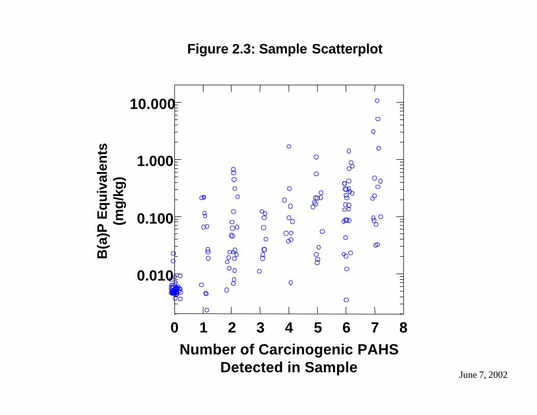
June 7, 2002

0 1 2 3 4 5 6 7 8

0.010

0.100

1.000

10.000

Figure 2.3: Sample Scatterplot

B(a

)P E

qu

ival

ents

(mg

/kg

)

Number of Carcinogenic PAHSDetected in Sample

June 7, 2002

Figure 2.4: Sample Probability Plot of Normal Fit to Data

0 5 10 15-3

-2

-1

0

1

2

3E

xpec

ted

Val

ue

B(a)P Equivalents (mg/kg)

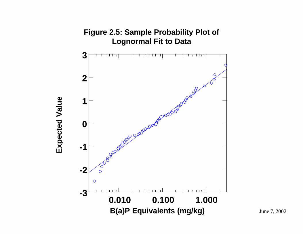
June 7, 2002

Figure 2.5: Sample Probability Plot of Lognormal Fit to Data

0.010 0.100 1.000-3

-2

-1

0

1

2

3E

xpec

ted

Val

ue

B(a)P Equivalents (mg/kg)

June 7, 2002

June 7, 2002

Figure 4.1: Box and Whisker Plot by Site -156 Samples

Chico

Colusa

Eureka

Hollister

Marysville

Monterey

Oak Knoll M

e

Oakdale

Oakland

Petaluma

Potrero

Redding

Salinas

San Luis Obi

Santa Cruz

St. Helena

Stockton

Watsonville

Willows

Site

0.010

0.100

1.000

10.000B

(a)P

Eq

uiv

alen

ts (

mg

/kg

)

Fresno 1 & 2

Midway Village

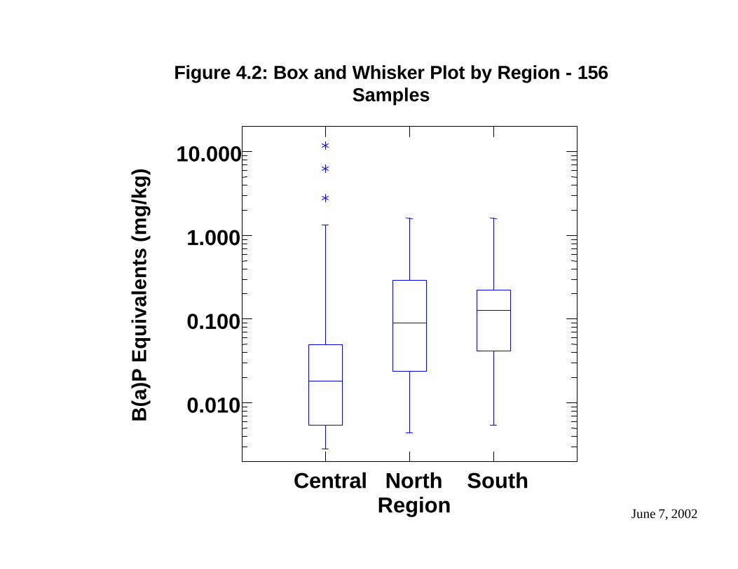
June 7, 2002

Figure 4.2: Box and Whisker Plot by Region - 156 Samples

Central North SouthRegion

0.010

0.100

1.000

10.000B

(a)P

Eq

uiv

alen

ts (

mg

/kg

)

June 7, 2002

Figure 4.3: Box and Whisker Plot by Proximity to Ocean - 156 Samples

No YesCoastal Site?

0.010

0.100

1.000

10.000

B(a

)P E

qu

ival

ents

(m

g/k

g)

June 7, 2002

0 1 2 3 4 5 6 7 8

0.010

0.100

1.000

10.000

Figure 4.4: Scatterplot of B(a)P Equivalent Concentrations versus Number of Detected Constituents - 156 Samples

B(a

)P E

qu

ival

ents

(m

g/k

g)

Number of Carcinogenic PAHsDetected in a Sample

June 7, 2002

Figure 4.5: Probability Plot of Normal Fit to Raw Data - 156 Samples

0 5 10 15-3

-2

-1

0

1

2

3

B(a)P Equivalents (mg/kg)

Exp

ecte

d V

alu

eCensored Samples

Non-Censored Samples

June 7, 2002

Figure 4.6: Probability Plot of Normal Fit to Log Transformed Data - 156 Samples

0.010 0.100 1.000 10.000-3

-2

-1

0

1

2

3E

xpec

ted

Val

ue

B(a)P Equivalents (mg/kg)

Censored Samples

Non-Censored Samples

June 7, 2002

Figure 5.1: Box and Whisker Plot by Site - 86 Samples

Chico

Colusa

Eureka

Hollister

Marysville

Monterey

Oak Knoll M

e

Oakdale

Oakland

Petaluma

Potrero

Redding

Salinas

San Luis Obi

Santa Cruz

St. Helena

Stockton

Watsonville

Willows

Site

0.010

0.100

1.000

B(a

)P E

qu

ival

ents

(m

g/k

g)

Fresno 1 & 2

Midway Village

June 7, 2002

Central North SouthRegion

0.010

0.100

1.000B

(a)P

Eq

uiv

alen

ts (

mg

/kg

)

Figure 5.2: Box and Whisker Plot by Region - 86 Samples

June 7, 2002

No Yes

0.010

0.100

1.000B

(a)P

Eq

uiv

alen

ts (

mg

/kg

)

Figure 5.3: Box and Whisker Plot by Proximity to Ocean - 86 Samples

Coastal Site ?

June 7, 2002

Figure 5.4: Probability Plot of Normal Fit to Data - 86 Samples

0 1 2 3-3

-2

-1

0

1

2

3E

xpec

ted

Val

ue

B(a)P Equivalents (mg/kg)

Censored Samples

Non-Censored Samples

June 7, 2002

Figure 5.5: Probability Plot of Lognormal Fit to Data - 86 Samples

0.010 0.100 1.000-3

-2

-1

0

1

2

3E

xpec

ted

Val

ue

B(a)P Equivalents (mg/kg)

Censored Samples

Non-Censored Samples

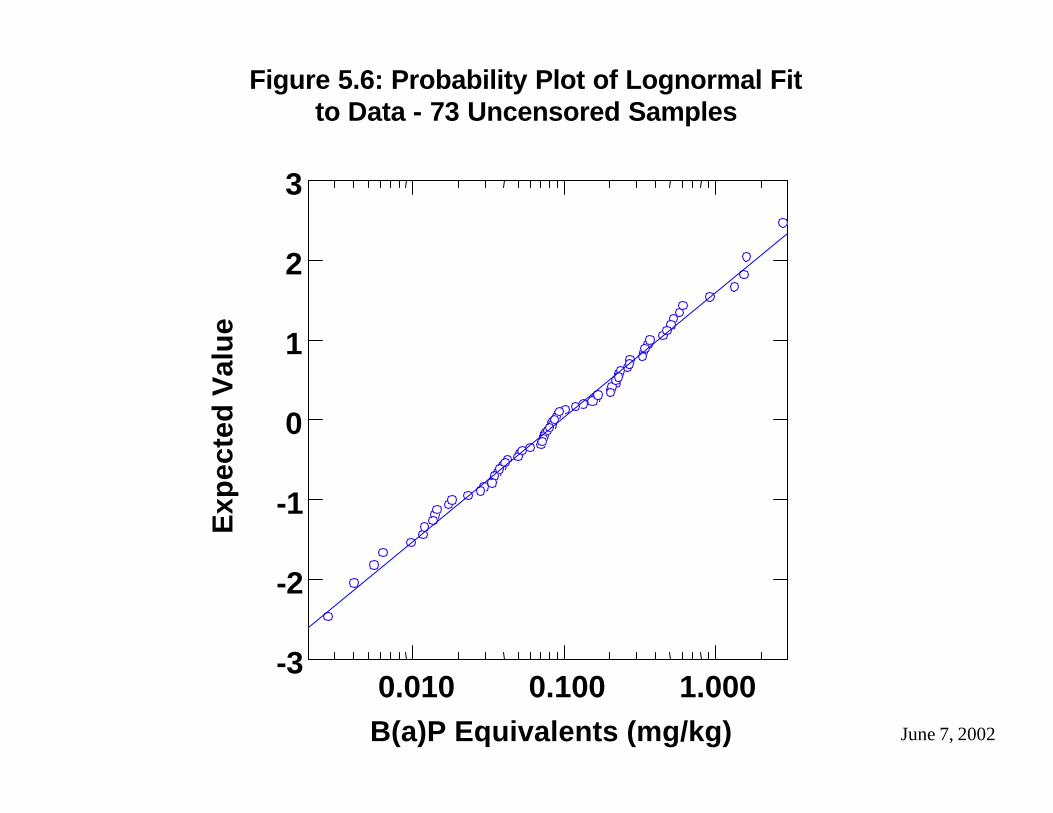
June 7, 2002

Figure 5.6: Probability Plot of Lognormal Fit to Data - 73 Uncensored Samples

0.010 0.100 1.000-3

-2

-1

0

1

2

3E

xpec

ted

Val

ue

B(a)P Equivalents (mg/kg)

June 7, 2002

Figure 5.7: Probability Plot of Lognormal Fit to Data - 86 Samples After Smoothing

0.010 0.100 1.000-3

-2

-1

0

1

2

3E

xpec

ted

Val

ue

B(a)P Equivalents (mg/kg)

Censored Samples

Non-Censored Samples

A-1 June 7, 2002

APPENDICES

Appendix A Printed Copy of Final Data Set

Appendix B Disk with Electronic Copies of Initial, Interim, and Final Data Sets

Appendix C Lab Sheets for Data Considered For or Included in Data Set

A-1 June 7, 2002

APPENDIX A

Final Data Set

Site Owner Site Name Sample ID

Total PAHs(mg/kg wet

weight)

Final 86 Sample Data Set Prior to Smoothing

B(a)P Equivalent(mg/kg wet weight)

Final 86 Sample** Smoothed Data Set B(a)P Equivalent

(mg/kg wet weight)PG&E Chico DSS-CHI1-10 8.1693 0.5281 0.5281PG&E Chico DSS-CHI1-6 46.5645 0.9209 0.9209PG&E Chico DSS-CHI1-7 1.4790 0.0299 0.0299PG&E Chico DSS-CHI1-8 5.5918 0.0755 0.0755PG&E Chico DSS-CHI1-9 7.4574 0.4484 0.4484PG&E Colusa DSS-COL-10 3.8003 0.3349 0.3349PG&E Colusa DSS-COL-7 2.3472 0.2040 0.2040PG&E Colusa DSS-COL-8 2.7454 0.0513 0.0513PG&E Colusa DSS-COL-9 11.2570 0.2724 0.2724PG&E Colusa2000 CS-1 0.0805 0.0077 0.0176PG&E Colusa2000 CS-2 0.0575 0.0055 0.0121PG&E Colusa2000 CS-3 0.0880 0.0055 0.0111PG&E Colusa2000 CS-4 0.1075 0.0077 0.0164PG&E Colusa2000 CS-5 0.4970 0.0118 0.0118PG&E Eureka SS-EKA-16 1.5087 0.0748 0.0748PG&E Eureka SS-EKA-17 1.7804 0.0931 0.0931PG&E Fresno-1 DSS-8 1.3511 0.1350 0.1350PG&E Fresno-2 DSS-FRS2-8 1.9809 0.2613 0.2613PG&E Fresno-2 DSS-FRS2-9 1.4255 0.2192 0.2192PG&E Hollister DSS-HOL-10 6.1829 0.5069 0.5069PG&E Hollister DSS-HOL-11 0.8319 0.0710 0.0710PG&E Hollister DSS-HOL-12 0.6104 0.0427 0.0427PG&E Hollister DSS-HOL-8 0.6421 0.0368 0.0368PG&E Hollister DSS-HOL-9 4.3980 0.1623 0.1623PG&E Marysville DSS-MRY1-4 14.5480 1.6116 1.6116PG&E Marysville DSS-MRY1-6 1.2488 0.0345 0.0345PG&E Marysville DSS-MRY1-8 1.2315 0.0283 0.0283

Midway Village Public Housing Midway-Bayshore BS-5 0.4618 0.0142 0.0142Midway Village Public Housing Midway-Bayshore BS-8 1.0171 0.0846 0.0846San Mateo County Housing Authority Midway Village2000 M101S 0.0403 0.0063 0.0063San Mateo County Housing Authority Midway Village2000 M140S 0.0225 0.0055 0.0101San Mateo County Housing Authority Midway Village2000 M70S 0.0225 0.0055 0.0092San Mateo County Housing Authority Midway Village2000 M95S 0.0225 0.0055 0.0082

PG&E Monterey DSS-MNT1-10 11.7284 1.5494 1.5494PG&E Monterey DSS-MNT1-11 1.5183 0.2067 0.2067PG&E Monterey DSS-MNT1-7 0.7374 0.1206 0.1206PG&E Monterey DSS-MNT1-8 0.9022 0.0740 0.0740PG&E Monterey DSS-MNT1-9 1.6533 0.2198 0.2198

U.S. Navy Oak Knoll Medical 029-SEW-1 0.3761 0.0138 0.0138PG&E Oakdale DSS-OKD-6 0.7318 0.0234 0.0234PG&E Oakdale DSS-OKD-7 1.7476 0.0840 0.0840PG&E Oakdale DSS-OKD-8 0.5567 0.0396 0.0396PG&E Oakdale DSS-OKD-9 0.2458 0.0121 0.0121PG&E Oakland DSS-OAK-10 1.3315 0.2312 0.2312PG&E Oakland DSS-OAK-11 6.5249 1.3387 1.3387PG&E Oakland DSS-OAK-7 3.3970 0.3588 0.3588PG&E Oakland DSS-OAK-8 16.1145 0.5804 0.5804PG&E Petaluma SS-PET-15 0.6434 0.0350 0.0350PG&E Potrero BSS-POT-1 2.2723 0.2354 0.2354PG&E Potrero BSS-POT-2 4.7292 0.2284 0.2284PG&E Potrero BSS-POT-3 2.4169 0.1550 0.1550PG&E Redding BG-14 2.9441 0.3285 0.3285

Final Data Set

Site Owner Site Name Sample ID

Total PAHs(mg/kg wet

weight)

Final 86 Sample Data Set Prior to Smoothing

B(a)P Equivalent(mg/kg wet weight)

Final 86 Sample** Smoothed Data Set B(a)P Equivalent

(mg/kg wet weight)

PG&E Redding BG-17 0.0400 0.0044 0.0037PG&E Redding BG-9 0.2809 0.0146 0.0146PG&E Redding REDSS3200 1.1087 0.0720 0.0720PG&E Redding REDSS3300 0.8167 0.0500 0.0500PG&E Redding SS-RED-5 1.5692 0.0900 0.0900PG&E Salinas DSS-SAL-7 0.0760 0.0070 0.0153PG&E Salinas DSS-SAL-9 2.3385 0.2703 0.2703PG&E San Luis Obispo DSS-SLO1-10 0.6774 0.0785 0.0785PG&E San Luis Obispo DSS-SLO1-11 2.0163 0.2024 0.2024PG&E San Luis Obispo DSS-SLO1-9 1.2218 0.1688 0.1688PG&E Santa Cruz LB-5 1.8627 0.0532 0.0532PG&E Santa Cruz RS-6A 0.3971 0.0099 0.0099PG&E Santa Cruz RS-6B 0.3505 0.0055 0.0073PG&E Santa Cruz RS-6C 0.1173 0.0055 0.0055PG&E Santa Cruz RS-8 0.1750 0.0055 0.0064PG&E Santa Cruz RS-9A 0.0575 0.0055 0.0055PG&E Santa Cruz RS-9B 0.0575 0.0055 0.0046PG&E St. Helena DBS-STH-1 1.5159 0.0027 0.0027PG&E St. Helena DBS-STH-2 1.2886 0.0878 0.0878PG&E St. Helena DBS-STH-3 6.0314 0.0174 0.0174PG&E St. Helena DBS-STH-4 3.7171 0.1026 0.1026PG&E St. Helena DBS-STH-5 0.7691 0.0041 0.0041PG&E Stockton SS-06 21.5224 2.8134 2.8134PG&E Stockton SS-07 3.0248 0.3688 0.3688PG&E Stockton SS-09 5.2757 0.6109 0.6109PG&E Watsonville DSS-WAT1-6 2.3682 0.3437 0.3437PG&E Watsonville DSS-WAT1-7 0.6525 0.0601 0.0601PG&E Watsonville DSS-WAT1-8 0.5406 0.0338 0.0338PG&E Watsonville DSS-WAT1-9 0.7146 0.0379 0.0379PG&E Willows DSS-WIL-10 3.9783 0.0808 0.0808PG&E Willows DSS-WIL-6 4.3379 0.4770 0.4770PG&E Willows DSS-WIL-7 0.5568 0.0184 0.0184PG&E Willows DSS-WIL-8 2.5340 0.0937 0.0937PG&E Willows DSS-WIL-9 3.7446 0.0411 0.0411

Notes/Data Codes:** - The only differences between the final 86 sample data set and the 86 sample data set prior to and after smoothing are the 13 smoothed results (highlighted data). As discussed in the text, these 13 samples were classified as censored samples.

= a smoothed result used to represent a censored data point.Bold Italics = Indicates values obtained by smoothing and associated with censored samples for which the original values were tied. As discussed in the text, individual values obtained by smoothing, cannot be assigned to specific censored samples. It should be noted that it is appropriate to use these values to calculate summary statistics, but these values should not be used when evaluating the differences among subsets of background data (e.g., subsets defined by site or region). These values have been listed with specific samples for the sole purpose of keeping the table format consistent.Bold Results = Indicates values obtained by smoothing and associated with censored samples for which the original values were not tied. Unlike the smoothed values associated with censored results which were tied, these results are not arbitrary and can be assigned to specific samples. For this reason, these values can be used when evaluating the differences among subsets of background data (e.g., subsets defined by site or region).

A-2 June 7, 2002

APPENDIX B

A-3 June 7, 2002

APPENDIX C