Embed Size (px)
Citation preview

Darboux Transformations, Discrete
Integrable Systems
and Related Yang-Baxter Maps
Sotiris Konstantinou-Rizos
Department of Applied Mathematics
University of Leeds
Submitted in accordance with the requirements for the degree of Doctor
of Philosophy
April 2014


The candidate confirms that the work submitted is his own, except where
work which has formed part of jointly-authored publications has been
included. The contribution of the candidate and the other authors to this
work has been explicitly indicated below. The candidate confirms that
appropriate credit has been given within the thesis where reference has
been made to the work of others.
• Chapter 5 is based on S. Konstantinou-Rizos and A.V. Mikhailov, “Darboux trans-
formations, finite reduction groups and related Yang-Baxtermaps”, Journal of
Physics A46 (2013), 425201.
The construction of Yang-Baxter maps by matrix refactorisation problems of Darboux
matrices was my original idea which we accomplished with theco-author, A.V. Mikha-
ilov, for all the cases of finite reduction groups with two-dimensional representation. The
contribution was equal. Moreover, I wrote the first draft of the paper which, after the
co-author’s amendments, was brought to a publishable form.
This copy has been supplied on the understanding that it is copyright
material and that no quotation from the thesis may be published without
proper acknowledgement.
c© 2014 The University of Leeds and Sotiris Konstantinou-Rizos

To my parents, Anastasia and Giorgos


AcknowledgementsDoing a PhD is a hard job, but at the same time it can become a pleasant experience if
you have the right people around you. Therefore, from this position, I would like to thank
all the people who contributed –one way or another– to makingit happen.
Above all, I would like to thank my supervisor, Alexander Mikhailov, for his guidance
and for being patient throughout my PhD studies. He has the experience and ability to
tell you straightaway if your ideas can work, which is very useful for a research student.
Moreover, he encouraged me to participate in many conferences from which I benefited
a lot. His constructive criticism on my research made me mature as a mathematician and
for that I am most grateful. At this point, I would also like tothank my adviser, Frank
Nijhoff, for his interest and for setting the guidelines in our yearly meetings.
I am greatly indebted to the University of Leeds for grantingme the William Wright Smith
scholarship and to J.E. Crowther for the scholarship-contribution to fees. Moreover, I
extend grateful thanks to the school of Mathematics for the financial support during my
writing-up period and for financing all the conferences in which I participated; I feel that
it was the ideal enviroment for postgraduate studies, in a very well-organised University
which I would highly recommend to any graduate student. It was also very beneficial to
be part of the integrable systems group, with weekly seminars and many other research
activities. Many thanks are also due to Alastair Rucklidge and Jeanne Shuttleworth for
welcoming me here in the school and for being very helpful over these years.
However, my postgraduate studies started in Greece, at the Univeristy of Patras, and
therefore there are several people who contributed to building my maths background.
First of all, I was very lucky to do my Master’s thesis under the supervision of Dimitris
Tsoubelis. He is the person who introduced me to the theory ofPDEs and, in general, to
Mathematical Physics, and he has been an enormous source of knowledge and experience
for me ever since. But more importantly, he taught me how to study mathematics myself,
how to write mathematical texts and research proposals and several other things which I
use daily in my research. Working with him is a pleasure, and he is a person who I always
seek advice from at any stage of my career. Therefore, I wouldlike to thank him for

supporting my studies in several ways. He and his wife, Eudokia Papafotopoulou, have
been very kind to me and for that I am most grateful.
I would also like to thank Vassilis Papageorgiou for his interest throughout these years and
for contributing into building my theoretical background during both my undergraduate
and postgraduate studies. He is always happy to discuss mathematics with me and he is
always willing to help me. Moreover, he and his wife, Eugenie Foustoucos, had helped
me to come here in Leeds in the beginning of my studies for which I am very grateful as
well as for their continuous interest in my progress.
Moreover, I would not be able to start my PhD studies without the help of Tolis Fasois
who prepared me for the IELTS exam. His job was difficult, as there were only a few days
before the exams; yet, he managed to improve my English in no time and I would like to
thank him from this position.
The person who introduced me into the theory of Yang-Baxter maps –which covers
a big part of this thesis– is Thodoris Kouloukas. We have had endless mathematical
conversations and I would like to thank him for that, as well as for being a very good
friend over these years. Many thanks are also due to my ex-neighbour and friend Georgi
Grahovski for explaining to me what a Grassmann algebra is and for being very helpful
during his postdoctoral stay in the University of Leeds. Moreover, I would like to thank
my academic brother and friend, George Berkeley, for readingmy thesis and making
comments on it. It has been very nice working with both of them. It was also very
beneficial to have several maths discussions with Pavlos Kassotakis, thus I would like to
thank him for that.
Pavlos Xenitidis and Anastasia Kazaltzi have been my familyhere in Leeds. I met them
in Patras when Pavlos was my academic tutor and they have beenmore than great friends
ever since. I came to Leeds one year after they moved here whenI decided to “follow”
them. Living in Leeds without them would be completely different, as they made me feel
as if I were home when I was away from it. I would like to thank them for everything
from this position.
I was also very lucky, since Ilia Roustemoglou decided to joinus one year after, and also
Giorgos Papamikos a bit after her. They are both long-time friends of mine and it was a

pleasure to have them around. Therefore, I would like to thank them for the nice time we
had in the UK. Additionally, I would like to thank Giorgos forproof-reading my thesis.
My postgraduate studies would never be the same without the support of my friends
Eleni Christodoulidi, Spiros Dafnis, Stelios “Spawn” Dimas, Nikos Kallinikos, Chrysavgi
Kostopoulou, Akis Matzaris, Mitsos Nomikos, Nikitas Nikandros, Grigoris Protsonis,
Panagiotis Protsonis and Stavros Anastasiou. At this point, I should extend many thanks
to Panagis Karazeris for being patient and friendly to all ofus. Additionally, I would also
like to thank Giota Adamopoulou and Maura Capuzzo who are the “new entries” in our
friends list. I would like to thank all the former for having an amazing time throughout
these years (and they are quite a few!) and for making the daily routine a pleasant journey.
Moreover, I had a really nice time with my PhD-fellows and friends Laurence Hawke,
Vijay Teeluck, Julia Sauter, Lamia Alqahtani, Neslihan Delice, Abeer Al-Nahdi, Huda
Alshanabari, Bartosz Szczesny, Gareth Hurst and all the restof the people in the satellite
postgraduate office. And, of course, special thanks to Ms Charikleia for cooking for
all of us. Finally, living in a shared flat would never be the same without the pleasant
company of my flatmates and very good friends Sophia-Marie Honny, Priya Sinha and
Moa Nasstrom.
Special thanks are due to my long-time friends Christos Fokas, Giorgos Panagiotidis in
Athens and Costantinos Balamoshev and Ewa Golic in Warsaw, whoI always think of no
matter how far away they are.
Finally, I am more than grateful to my parents Anastasia and Giorgos for supporting
everything I choose to do in my life. Moreover, special thanks to my uncle and aunt,
Charilaos and Aleka, for their interest and support and to allthe rest of the family but
especially my twin brother Michael and my cousins and friends Costas, Stelios, Zoe and
Marianna who I grew up with.

i
AbstractDarboux transformations constitute a very important tool in the theory of integrable
systems. They map trivial solutions of integrable partial differential equations to non-
trivial ones and they link the former to discrete integrablesystems. On the other hand,
they can be used to construct Yang-Baxter maps which can be restricted to completely
integrable maps (in the Liouville sense) on invariant leaves.
In this thesis we study the Darboux transformations relatedto particular Lax operators
of NLS type which are invariant under the action of the so-called reduction group.
Specifically, we study the cases of: 1) the nonlinear Schrodinger equation (with no
reduction), 2) the derivative nonlinear Schrodinger equation, where the corresponding
Lax operator is invariant under the action of theZ2-reduction group and 3) a deformation
of the derivative nonlinear Schrodinger equation, associated to a Lax operator invariant
under the action of the dihedral reduction group. These reduction groups correspond to
recent classification results of automorphic Lie algebras.
We derive Darboux matrices for all the above cases and we use them to construct
novel discrete integrable systems together with their Lax representations. For these
systems of difference equations, we discuss the initial value problem and, moreover,
we consider their integrable reductions. Furthermore, thederivation of the Darboux
matrices gives rise to many interesting objects, such as Backlund transformations for the
corresponding partial differential equations as well as symmetries and conservation laws
of their associated systems of difference equations.
Moreover, we employ these Darboux matrices to construct six-dimensional Yang-Baxter
maps for all the afore-mentioned cases. These maps can be restricted to four-dimensional
Yang-Baxter maps on invariant leaves, which are completely integrable; we also consider
their vector generalisations.
Finally, we consider the Grassmann extensions of the Yang-Baxter maps corresponding
to the nonlinear Schrodinger equation and the derivative nonlinear Schrodinger equation.
These constitute the first examples of Yang-Baxter maps with noncommutative variables
in the literature.

ii

iii
Contents
Abstract . . . . . . . . . . . . . . . . . . . . . . . . . . . . . . . . . . . . . . i
Contents . . . . . . . . . . . . . . . . . . . . . . . . . . . . . . . . . . . . . . iii
List of abbreviations . . . . . . . . . . . . . . . . . . . . . . . . . . . . . . . viii
List of figures . . . . . . . . . . . . . . . . . . . . . . . . . . . . . . . . . . . xi
1 Introduction 1
1.1 Lax representations and the IST . . . . . . . . . . . . . . . . . . . . .. 2
1.1.1 Lax representations . . . . . . . . . . . . . . . . . . . . . . . . . 3
1.1.2 The inverse scattering transform . . . . . . . . . . . . . . . . .. 5
1.1.3 The AKNS scheme . . . . . . . . . . . . . . . . . . . . . . . . . 6
1.2 Discrete integrable systems . . . . . . . . . . . . . . . . . . . . . . .. . 7
1.2.1 Equations on Quad-Graphs: 3D-consistency . . . . . . . . .. . . 8
1.2.2 ABS classification of maps on quad-graphs . . . . . . . . . . . .10
1.2.3 Classification of quadrirational maps: TheF -list . . . . . . . . . 11
1.3 Organisation of the thesis . . . . . . . . . . . . . . . . . . . . . . . . .. 12
2 Backlund and Darboux transformations 15
2.1 Overview . . . . . . . . . . . . . . . . . . . . . . . . . . . . . . . . . . 15
2.2 Darboux transformations . . . . . . . . . . . . . . . . . . . . . . . . . .16

CONTENTS iv
2.2.1 Darboux’s theorem . . . . . . . . . . . . . . . . . . . . . . . . . 16
2.2.2 Darboux transformation for the KdV equation and Crum’stheorem 17
2.3 Backlund transformations . . . . . . . . . . . . . . . . . . . . . . . . . . 19
2.3.1 BT for sine-Gordon equation and Bianchi’s permutability . . . . . 21
2.3.2 Backlund transformation for the PKdV equation . . . . . . . . . 24
3 Darboux tranformations for NLS type equations and discrete integrable
systems 27
3.1 Overview . . . . . . . . . . . . . . . . . . . . . . . . . . . . . . . . . . 27
3.2 The reduction group and automorphic Lie algebras . . . . . .. . . . . . 29
3.3 General framework . . . . . . . . . . . . . . . . . . . . . . . . . . . . . 30
3.3.1 Derivation of Darboux matrices . . . . . . . . . . . . . . . . . . 30
3.3.2 Discrete Lax pairs and discrete systems . . . . . . . . . . . .. . 34
3.4 NLS type equations . . . . . . . . . . . . . . . . . . . . . . . . . . . . . 38
3.4.1 The nonlinear Schrodinger equation . . . . . . . . . . . . . . . . 38
3.4.2 The derivative nonlinear Schrodinger equation:Z2-reduction group 41
3.4.3 A deformation of the derivative nonlinear Schrodinger equa-
tion: Dihedral reduction group . . . . . . . . . . . . . . . . . . . 45
3.5 Derivation of discrete systems and initial value prob-
lems . . . . . . . . . . . . . . . . . . . . . . . . . . . . . . . . . . . . . 49
3.5.1 Nonlinear Schrodinger equation and related discrete systems . . . 49
3.5.2 Derivative nonlinear Schrodinger equation and related discrete
systems . . . . . . . . . . . . . . . . . . . . . . . . . . . . . . . 54
3.5.3 A deformation of the derivative nonlinear Schrodinger equa-
tion and related discrete systems . . . . . . . . . . . . . . . . . . 57

CONTENTS v
4 Introduction to Yang-Baxter maps 63
4.1 Overview . . . . . . . . . . . . . . . . . . . . . . . . . . . . . . . . . . 63
4.2 The quantum Yang-Baxter equation . . . . . . . . . . . . . . . . . . . .64
4.2.1 Parametric Yang-Baxter maps . . . . . . . . . . . . . . . . . . . 64
4.2.2 Matrix refactorisation problems and the Lax equation. . . . . . . 66
4.3 Yang-Baxter maps and 3D consistent equations . . . . . . . . . .. . . . 69
4.4 Classification of quadrirational YB maps: TheH-list . . . . . . . . . . . 70
4.5 Transfer dynamics of YB maps and initial value pro-
blems . . . . . . . . . . . . . . . . . . . . . . . . . . . . . . . . . . . . 72
5 Yang-Baxter maps related to NLS type equations 75
5.1 Overview . . . . . . . . . . . . . . . . . . . . . . . . . . . . . . . . . . 75
5.2 Preliminaries . . . . . . . . . . . . . . . . . . . . . . . . . . . . . . . . 76
5.2.1 Poisson manifolds and Casimir functions . . . . . . . . . . . .. 76
5.2.2 Properties of the YB maps which admit Lax representation . . . . 77
5.2.3 Liouville integrability of Yang-Baxter maps . . . . . . . .. . . . 79
5.3 Derivation of Yang-Baxter maps . . . . . . . . . . . . . . . . . . . . . .80
5.3.1 The Nonlinear Schrodinger equation . . . . . . . . . . . . . . . . 81
5.3.2 Derivative NLS equation:Z2 reduction . . . . . . . . . . . . . . 84
5.3.3 A deformation of the DNLS equation: Dihedral Group . . .. . . 89
5.3.4 Dihedral group: A linearised YB map . . . . . . . . . . . . . . . 92
5.4 2N × 2N -dimensional YB maps . . . . . . . . . . . . . . . . . . . . . . 92
5.4.1 NLS equation . . . . . . . . . . . . . . . . . . . . . . . . . . . . 93
5.4.2 Z2 reduction . . . . . . . . . . . . . . . . . . . . . . . . . . . . 94

CONTENTS vi
6 Extensions on Grassmann algebras 95
6.1 Overview . . . . . . . . . . . . . . . . . . . . . . . . . . . . . . . . . . 95
6.2 Elements of Grassmann algebras . . . . . . . . . . . . . . . . . . . . .. 96
6.2.1 Supertrace and superdeterminant . . . . . . . . . . . . . . . . .. 97
6.2.2 Differentiation rule for odd variables . . . . . . . . . . . .. . . . 97
6.2.3 Properties of the Lax equation . . . . . . . . . . . . . . . . . . . 98
6.3 Extensions of Darboux transformations on Grass-
mann algebras . . . . . . . . . . . . . . . . . . . . . . . . . . . . . . . . 99
6.3.1 Nonlinear Schrodinger equation . . . . . . . . . . . . . . . . . . 100
6.3.2 Derivative nonlinear Schrodinger equation . . . . . . . . . . . . . 102
6.4 Grassmann extensions of Yang-Baxter maps . . . . . . . . . . . . .. . . 105
6.4.1 Nonlinear Schrodinger equation . . . . . . . . . . . . . . . . . . 105
6.4.2 Derivative nonlinear Schrodinger equation . . . . . . . . . . . . . 108
6.4.3 Restriction on invariant leaves . . . . . . . . . . . . . . . . . . .109
6.5 Vector generalisations:4N × 4N Yang-Baxter maps . . . . . . . . . . . 112
6.5.1 Nonlinear Schrodinger equation . . . . . . . . . . . . . . . . . . 112
6.5.2 Derivative nonlinear Schrodinger equation . . . . . . . . . . . . . 113
7 Conclusions 115
7.1 Summary of results . . . . . . . . . . . . . . . . . . . . . . . . . . . . . 115
7.2 Future work . . . . . . . . . . . . . . . . . . . . . . . . . . . . . . . . . 116
Appendix 119
A Solution of the system of discrete equations associated tothe deformation
of the DNLS equation . . . . . . . . . . . . . . . . . . . . . . . . . . . . 119

CONTENTS vii
Bibliography 121
Index 129

CONTENTS viii

ix
List of abbreviations
ABS Adler, Bobenko and Suris
AKNS Ablowitz, Kaup, Newell and Segur
BT Backlund transformation
DNLS Derivative nonlinear Schrodinger
dpKdV discrete potential Korteweg-de Vries
DT Darboux transformation
GGKM Gardner, Greene, Kruskal and Miura
IST Inverse scattering transform
KdV Korteweg de Vries
NLS Nonlinear Schrodinger
ODE Ordinary differential equation
PDE Partial differential equation
PKDV Potential Korteweg de Vries
SG sine-Gordon
YB Yang-Baxter

List of abbreviations x

xi
List of figures
1.1 IST scheme . . . . . . . . . . . . . . . . . . . . . . . . . . . . . . . . . 6
1.2 3D-consistency. . . . . . . . . . . . . . . . . . . . . . . . . . . . . . . . 9
2.1 Bianchi’s permutability . . . . . . . . . . . . . . . . . . . . . . . . . . .23
3.1 Bianchi commuting diagram . . . . . . . . . . . . . . . . . . . . . . . . 34
3.2 Initial value problem and direction of evolution . . . . . .. . . . . . . . 51
3.3 The stencil of six points and the initial value problem for equation (3.109). . . 56
3.4 The stencil of seven points and the initial value problem on the black and white
lattice . . . . . . . . . . . . . . . . . . . . . . . . . . . . . . . . . . . . 61
4.1 Cubic representation of (a) the parametric YB map and (b) the
corresponding YB equation. . . . . . . . . . . . . . . . . . . . . . . . . 66
4.2 (a) dpKdV equation: fields placed on vertices (b) Adler’smap: fields
placed on the edges. . . . . . . . . . . . . . . . . . . . . . . . . . . . . . 70
4.3 Transfer maps corresponding to then-periodic initial value problem . . . 73

LIST OF FIGURES xii

1
Chapter 1
Introduction
The aim of this chapter is to give an introduction to the subject of integrable systems,
which forms the context of this thesis. Integrable systems arise in nonlinear processes
and, both in their classical and quantum version, have many applications in various fields
of mathematics and physics.
However, the definition of integrable systems is itself highly nontrivial; many scientists
have different opinions on what “integrable” should mean, which makes the definition
of integrability elusive, rather than tangible. In fact, a comprehensive definition of
integrability is not yet available. As working definitions we often use the existence of
a Lax pair, the solvability of the system by the IST, the existence of infinitely many
symmetries or conservation laws, or the existence of a sufficient number of first integrals
which are in involution (Liouville integrability); there is even a book entirely devoted to
what is integrability[94].
In this thesis we are interested in the derivation of discrete integrable systems and Yang-
Baxter maps, from (integrable) PDEs which admit Lax representation, via Darboux
transformations. Specifically, we shall be focusing on particular PDEs of NLS type whose
corresponding Lax operators possess certain symmetries, due to the action of the so-called
reduction group.
Since these AKNS-type Lax operators we are dealing with constitute a key role in the
integrability of their associated equations under the IST,the inverse scattering method and
Chapter 1. Introduction 2
the AKNS scheme deserve a few pages in the first part of this introduction. However, we
will skip the technical parts of their methods, as it is not the aim of this thesis. For detailed
information on the methods and the historical review of the results, we indicatively refer
to [4, 1, 31] (and the references therein).
The second part of this chapter is devoted to a brief introduction to the integrability
of discrete systems; in the main, their multidimensional consistency and some recent
classification results.
1.1 Lax representations and the IST
The inverse scattering transformation (or just transform)is a method for solving nonlinear
PDEs. Its name is due to the main idea of the method, namely therecovery of the time
evolution of the potential solution of the nonlinear equation, from the time evolution of
its scattering data. As a matter of fact, the method of the inverse scattering transform is of
the same philosophy as the Fourier transform technique for solving linear PDEs; actually,
the IST is also found in the literature as the nonlinear Fourier transform. However, it does
not apply to all nonlinear equations in a systematic way.
The first example of nonlinear PDE solvable by the IST method,is the KdV equation,
namely
ut = 6uux − uxxx, u = u(x, t), (1.1)
which is undoubtedly the most celebrated nonlinear PDE overthe last few decades. It
mostly owes its popularity to Gardner, Greene, Kruskal and Miura, who were the first
to derive the exact solution of the Cauchy problem for the KdV equation, for rapidly
decaying initial values, in late sixties [36]. However, equation (1.1) was derived by
Diederik Korteweg and Gustav de Vries in 1895, as a mathematical model of water-waves
in shallow channels. In fact, they showed that the KdV equation represents Scott Russel’s
solitary wave, known assoliton (see [31] for details). The name “soliton” was given
by Zabusky and Kruskal1 in 1965, when they discovered numerically that these wave
1They initially called it “solitron”, but at the same time a company was trading with the same name and
therefore had to remove the “r”.

Chapter 1. Introduction 3
solutions behave like particles; they retain their amplitude and speed after collision.
The work of GGKM in 1967, namely the IST method, is probably one of the most
significant results of the last century in the theory of nonlinear PDEs. It is not only a
technique for solving the initial value problem for KdV, butit also initiated a more general
scheme applicable to other nonlinear PDEs. In fact, P. Lax was the one who contributed
in this direction, formulating a more general framework a year later in [55].
1.1.1 Lax representations
Lax’s generalisation concerns nonlinearevolution equations, namely equations of the
form
ut = N(u), u = u(x, t), (1.2)
whereN is a nonlinear differential operator, which does not dependon∂t.
In particular, Lax considered a pair of linear differentialoperators,L andA. OperatorL
is associated to the following spectral problem of finding eigenvalues and eigenfunctions
Lψ = λψ, ψ = ψ(x, t) (1.3a)
whileA is the operator related to the time evolution of the eigenfunctions
ψt = Aψ. (1.3b)
Proposition 1.1.1 (Lax’s equation) If the spectral parameter does not evolve in time,
namelyλt = 0, then relations (1.3) imply
Lt + [L,A] = 0, (1.4)
where[L,A] := LA−AL.
Proof
Differentiation of (1.3a) with respect tot implies
Ltψ + Lψt = λψt. (1.5)

Chapter 1. Introduction 4
Using both relations (1.3), the above equation can be rewritten as
(Lt + LA−AL)ψ = 0. (1.6)
Now, since the above holds for the arbitrary eigenfunctionψ(x, t), it implies equation
(1.4).✷
If a nonlinear evolution equation (or a system of equations)of the form (1.2) is equivalent
to (1.4), then we can associate to it a pair of linear operators as (1.3). In this case, equation
(1.4) is called theLax equation, while equations (1.3) constitute aLax representationor,
simply, aLax pair for (1.2). In particular, equation (1.3a) is called thespatial partof the
Lax pair (orx-part), while equation (1.3b) is called itstemporal part(or t-part).
The property of a nonlinear evolution equation to be writtenas a compatibility condition
of a pair of linear equations (1.4) plays a key role towards the solvability of the equation
under the IST, and it is usually used as an integrability criterion.
Remark 1.1.2 For a given nonlinear evolution equation (1.2) there is no systematic
method of writing it as a compatibility condition of a pair oflinear equations, namely to
determine operatorsL andA. In fact, the usual procedure is to first study differential
operators of certain form, and then to examine what kind of PDEs result from their
compatibility condition.
Example 1.1.3 The KdV equation (1.1) can be written as a compatibility condition of the
form (1.4), of a system of linear equations (1.3), whereL andA are given by
L = −∂2x + u, u = u(x, t), (1.7a)
A = −4∂3x + 3u∂x + 3ux. (1.7b)
OperatorsL andA constitute a Lax pair for the KdV equation.
Operator (1.7a) is the so-called Schrodinger operator and the corresponding equation
Lψ = λψ is the time-independent Schrodinger equation, which constitutes a fundamental
equation in mathematical physics since the first quarter of the 20th century. However,

Chapter 1. Introduction 5
the Lax pair (1.7) for the KdV equation was not derived from the equation itself. As a
matter of fact, the “guess” of the operator (1.7a) was inspired by the desire to link the
KdV equation with Schrodinger’s equation.
We will come back to this Schrodinger equation in the next chapter, where we shall study
its covariance under the so-called Darboux transformation.
1.1.2 The inverse scattering transform
Although so far the method of the inverse scattering transform is not yet formulated to be
uniformly applicable to all nonlinear evolution equations, it always consists of three basic
steps. We briefly explain these steps, and we also present them schematically in Figure
1.1.
Consider the following Cauchy problem
ut = N(u), u(x, 0) = f(x), u := u(x, t), (1.8)
for a nonlinear evolution equation. Let us also assume that the above PDE admits Lax
representation (1.3).
StepI: The direct problem
The direct problem consists of finding the scattering transformation at a fixed value of the
temporal parameter, sayt = 0, by using the initial conditionu(x, 0) = f(x). That is to
find the spectral data of operatorL, which are called thescattering data. The scattering
transform att = 0 is nothing but a set of scattering data, which we denoteS(u)|t=0.
StepII: Time evolution of the scattering data
This is the part where one needs to determine the scattering data at an arbitrary time
t ∈ R, i.e. givenS(u)|t=0, use the second equation of (1.3) to determineS(u)|t∈R. The
significance of this part lies in the fact that we are now dealing with a linear problem,
(1.3b), rather than a nonlinear one as the original.

Chapter 1. Introduction 6
StepIII: The inverse problem
Analogously to the Fourier transform method, the final step is to recoveru = u(x, t) from
S(u)|t∈R.
u(x, 0) u(x, t)
S(u)|t=0 S(u)|t∈R
I III
II
Nonlinear evolution
Scattering data evolution
Dire
ctpr
oble
m
Inve
rse
prob
lem
Figure 1.1: IST scheme
1.1.3 The AKNS scheme
In 1971 Zakharov and Shabat [93] applied the inverse scattering transform method to
solve the NLS equation, introducing a more general formulation than Lax’s. Specifically,
they introduced a pair of linear equations, namely
∂xψ = Lψ, ψ := ψ(x, t), (1.9a)
∂tψ = T ψ, (1.9b)
whereL = L(x, t;λ) andT = T (x, t;λ) are2× 2 matrices. They showed that the NLS
equation,
pt = pxx + 4p2q, qt = −qxx − 4pq2, (1.10)
can be written as a compatibility condition,ψxt = ψtx, of the system of linear equations
(1.9), whereL andT are given by
L = Dx + U, T = Dt + V, (1.11)

Chapter 1. Introduction 7
andU andV by
U = λσ3 +
0 2p
2q 0
, σ3 := diag(1,−1), (1.12a)
V = λ2σ3 + λ
0 2p
2q 0
+
−2pq px
−qx 2pq
. (1.12b)
A year later, Ablowitz, Kaup, Newell and Segur in [2], motivated by Zakharov and
Shabat’s result, solved the sine-Gordon equation and they generalised this method to
cover a wider number of nonlinear PDEs (see [3]). In the rest of this thesis, we shall
refer to operators of the form (1.11) asLax operators of AKNS-type.
1.2 Discrete integrable systems
Discrete systems, namely systems with their independent variables taking discrete values,
are of particular interest and have many applications in several sciences as physics,
biology, financial mathematics, as well as several other branches of mathematics, since
they are essential in numerical analysis. Initially, they were appearing as discretisations
of continuous equations, but now discrete integrable systems, and in particular those
defined on a two-dimensional lattice, are appreciated in their own right from a theoretical
perspective.
The study of discrete systems and their integrability earned its interest in late seventies;
Hirota studied particular discrete systems in 1977, in a series of papers [43, 44, 45, 46]
where he derived discrete analogues of many already famous PDEs. In the early eighties,
semi-discrete and discrete systems started appearing in field-theoretical models in the
work of Jimbo and Miwa; they also provided a method of generating discrete soliton
equations [24, 25, 26, 27, 28]. Shortly after, Ablowitz and Taha in a series of papers [84,
85, 86] are using numerical methods in order to find solutionsfor known integrable PDEs,
using as basis of their method some partial difference equations, which are integrable in
their own right. Moreover, Capel, Nijhoff, Quispel and collaborators provided some of
the first systematic tools for studying discrete integrablesystems and, in particular, for the
Chapter 1. Introduction 8
direct construction of integrable lattice equations (we indicatively refer to [70, 79]); that
was a starting point for new systems of discrete equations toappear in the literature.
In 1991 Grammaticos, Papageorgiou and Ramani proposed the first discrete integrability
test, known assingularity confinement[39], which is similar to that of the Painleve
property for continuous integrability. However, as mentioned in [40], it is not sufficient
criterion for predicting integrability, as it does not furnish any information about the rate
of growth of the solutions of the discrete integrable system.
As in the continuous case, the usual integrability criterion being used for discrete systems
is the existence of a Lax pair. Nevertheless, a very important integrability criterion is
that of the 3D-consistencyand, by extension, themultidimensional consistency. This was
proposed independently by Nijhoff in 2001 [72] and Bobenko and Suris in 2002 [15].
In what follows, we briefly explain what is the 3D-consistency property and we review
some recent classification results. For more information onthe integrability of discrete
systems we refer to [69] which is one of the few self-contained monographs, as well as
[40] for a collection of results.
1.2.1 Equations on Quad-Graphs: 3D-consistency
Let us consider a discrete equation of the form
Q(u, u10, u01, u11; a, b) = 0, (1.13)
whereuij, i, j = 0, 1, u ≡ u00, belong in a setA and the parametersa, b ∈ C. Moreover,
we assume that (1.13) is uniquely solvable for anyui in terms of the rest. We can interpret
the fieldsui to be attached to the vertices of a square as in Figure 1.2-(a).
If equation (1.13) can be generalised in a consistent way on the faces of a cube, then it
is said to be3D-consistent. In particular, suppose we have the initial valuesu, u100, u010
andu001 attached to the vertices of the cube as in Figure 1.2-(b). Now, since equation
(1.13) is uniquely solvable, we can uniquely determine valuesu110, u101 andu011, using
the bottom, front and left face of the cube. Then, there are three ways to determine value
u111, and we have the following.

Chapter 1. Introduction 9
Definition 1.2.1 If for any choice of initial valuesu, u100, u010 andu001, equationQ = 0
produces the same valueu111 when solved using the left, back or top face of the cube, then
it is called 3D-consistent.
u u10
u01 u11
a
a
b b
u u100
u110u010
u001 u101
u111u011
a
a
a
c
b b
c
(b) Cube(a) Quad-Graph
Figure 1.2: 3D-consistency.
Note 1.2.2 In the above interpretation, we have adopted the following notation: We
consider the square in Figure 1.2-(a) to be an elementary square in a two dimensional
lattice. Then, we assume that fieldu depends on two discrete variablesn andm, i.e.
u = u(n,m). Therefore,uijs on the vertices of 1.2-(a) are
u00 = u(n,m), u10 = u(n+ 1,m), u01 = u(n,m+ 1), u11 = u(n+ 1,m+ 1).
(1.14)
Moreover, for the interpretation on the cube we assume thatu depends on a third variable
k, such that
u000 = u(n,m, k), u100 = u(n+1,m, k), . . . u111 = u(n+1,m+1, k+1). (1.15)
Now, as an illustrative example we use the discrete potential KdV equation which first
appeared in [43].
Example 1.2.3 (Discrete potential KdV equation) Consider equation (1.13), whereQ is
given by
Q(u, u10, u01, u11; a, b) = (u− u11)(u10 − u01) + b− a. (1.16)

Chapter 1. Introduction 10
Now, using the bottom, front and left faces of the cube 1.2-(b), we can solve equations
Q(u, u100, u010, u110; a, b) = 0, (1.17a)
Q(u, u100, u001, u101; a, c) = 0, (1.17b)
Q(u, u010, u001, u011; b, c) = 0, (1.17c)
to obtain solutions foru110, u101 andu011, namely
u110 = u+a− b
u010 − u100, (1.18a)
u101 = u+a− c
u001 − u100, (1.18b)
u011 = u+b− c
u001 − u010, (1.18c)
respectively.
Now, if we shift (1.18a) in thek-direction, and then substituteu101 andu011 (which appear
in the resulting expression foru11) by (1.18), we deduce
u111 = −(a− b)u100u010 + (b− c)u010u001 + (c− a)u100u001
(a− b)u001 + (b− c)u100 + (c− a)u010. (1.19)
It is obvious that, because of the symmetry in the above expression, we would obtain
exactly the same expression foru111 if we had alternatively shiftedu101 in them-direction
and substitutedu110 andu011 by (1.18), or if we had shiftedu011 in then-direction and
substitutedu110 andu101. Thus, the dpKdV equation is 3D-consistent.
1.2.2 ABS classification of maps on quad-graphs
In 2003 [8] Adler, Bobenko and Suris classified all the 3D-consistent equations in the case
whereA = C. In particular, they considered all the equations of the form (1.13), where
u, u10, u01, u11, a, b∈ C, that satisfy the following properties:
(I) Multilinearity. FunctionQ = Q(u, u10, u01, u11; a, b) is a first order polynomial in
each of its arguments, namely linear in each of the fieldsu, u10, u01, u11. That is,
Q(u, u10, u01, u11; a, b) = a1uu10u01u11 + a2uu10u01 + a3uu10u11 + . . .+ a16, (1.20)
whereai = ai(a, b), i = 1, . . . , 16.

Chapter 1. Introduction 11
(II) Symmetry. FunctionQ satisfies the following symmetry property
Q(u, u10, u01, u11; a, b) = ǫQ(u, u01, u10, u11; b, a) = σQ(u10, u, u11, u01; a, b), (1.21)
with ǫ, σ = ±1.
(III) Tetrahedron property. That is, the final valueu111 is independent ofu.
ABS proved that all the equations of the form (1.13) which satisfy the above conditions,
can be reduced to seven basic equations, using Mobius (fraction linear) transformations
of the independent variables and point transformations of the parameters. These seven
equations are distributed into two lists known as theQ-list (list of 4 equations) and the
H-list (list of 3 equations).
Remark 1.2.4 The dpKdV equation in Example 4.24 is the fisrt member of theH-list
(H1 equation).
Lax representations
Those equations of the form (1.13) which satisfy the multilinearity condition (I), admit
Lax representation. In fact, in this case, introducing an auxiliary spectral parameter,λ,
there is an algorithmic way to find a matrixL such that equation (1.13) can be written as
the followingzero-curvatureequation
L(u11, u01; a, λ)L(u01, u; b, λ) = L(u11, u10; b, λ)L(u10, u; a, λ). (1.22)
We shall see later on that 1) equations of the form (1.13) withthe fields on the edges of
the square 1.2-(a) are related to Yang-Baxter maps and 2) Yang-Baxter maps may have
Lax representation as (1.22).
1.2.3 Classification of quadrirational maps: TheF -list
A year after the classification of the 3D-consistent equations, ABS in [9] classified all the
quadrirational maps in the case whereA = CP1; the associated list of maps is known as

Chapter 1. Introduction 12
theF -list. Recall that, a mapY : (x, y) 7→ (u(x, y), v(x, y)) is calledquadrirational, if
the maps
u(., y) : A → A, v(x, .) : A → A, (1.23)
are birational. In particular, we have the following.
Theorem 1.2.5 (ABS,F -list) Up to Mobius transformations, any quadrirational map on
CP1 × CP1 is equivalent to one of the following maps
u = ayP, v = bxP, P =(1− b)x+ b− a+ (a− 1)y
b(1− a)x+ (a− b)xy + a(b− 1)y; (FI)
u =y
aP, v =
x
bP, P =
ax− by + b− a
x− y; (FII)
u =y
aP, v =
x
bP, P =
ax− by
x− y; (FIII)
u = yP v = xP, P = 1 +b− a
x− y; (FIV )
u = y + P, v = x+ P, P =a− b
x− y, (FV )
up to suitable choice of the parametersa andb.
We shall come back to theF -list in chapter 4, where we shall see that all the equations
of theF -list have the Yang-Baxter property; yet, the other members of their equivalence
classes may not satisfy the Yang-Baxter equation. However, we shall present a more
precise list given in [75].
Finally, we devote the last part of this introduction to present the plan of this thesis.
1.3 Organisation of the thesis
The results of the thesis are distributed to chapters 3, 5 and6 and appear in the articles
[50], [49] and [37], respectively. The character of chapter2 is introductory, while chapter
4 is a review to recent developments in the area of Yang-Baxtermaps. Specifically, this
thesis is organised as follows.
Chapter 2 deals with Backlund and Darboux transformations. In particular, starting with
the original theorem of Darboux, that was presented in 1882 ([23]), we explain that a

Chapter 1. Introduction 13
Darboux transformation is nothing else but a transformation which leaves covariant a
Sturm-Liouville problem. We show that this fact can be used to construct hierarchies
of solutions of particular nonlinear equations and we present the very well-known
Darboux transformation for the KdV equation. Moreover, we explain what are Backlund
transformations, namely transformations which relate either solutions of a particular PDE
(auto-BT), or solutions of different PDEs (hetero-BT). We show how, using BTs, one
can construct solutions of a nonlinear PDE in an algebraic manner, and we present the
well-known examples of the BTs for the sine-Gordon equation and the KdV equation.
In chapter 3 we derive Darboux transformations for particular NLS type equations,
namely the NLS equation, the DNLS equation and a deformationof the DNLS equation.
The spatial parts of the Lax pair of these equations are represented by (Lax) operators
which possess certain symmetries; in particular, these symmetries are due to the action
of the reduction group. In all the afore-mentioned cases, wederive DTs which are
understood as gauge-like transformations which depend rationally on a spectral parameter
and inherit the symmetries of their corresponding Lax operator. These DTs are employed
in the construction of novel discrete integrable systems which have first integrals and, in
some cases, can be reduced to Toda type equations. Moreover,the derivation of the DT
implies other significant objects, such as Backlund transformations for the corresponding
PDEs, as well as symmetries and conservation laws for the associated discrete systems.
All these cases of NLS type equations studied in this chaptercorrespond to recent
classification results.
Chapter 4 has introductory character and it is devoted to Yang-Baxter maps. In particular,
we explain what Yang-Baxter maps are and what is their connection with matrix
refactorisation problems. Moreover, we show the relation between the YB equation and
3D consistency equations, plus we review some of the recent developments, such as the
associated transfer dynamics and some recent classification results.
In chapter 5 we employ the Darboux transformations –derived inchapter 3– in the
construction of Yang-Baxter maps, and we study their integrability as finite discrete
maps. Particularly, we construct six-dimensional YB maps which can be restricted to
four-dimensional YB maps which are completely integrable in the Liouville sense. These

Chapter 1. Introduction 14
integrable restrictions are motivated by the existence of certain first integrals. In the case
of NLS equation, the four-dimensional restriction is the Adler-Yamilov map.
Chapter 6 is devoted to the noncommutative extensions of both Darbouxtransformations
and Yang-Baxter maps in the cases of NLS and DNLS equations. Specifically, we
show that there are explicit Yang-Baxter maps with Darboux-Lax representation between
Grassman algebraic varieties. We deduce novel endomorphisms of Grassmann varieties
and, in particular, we present ten-dimensional maps which can be restricted to eight-
dimensional Yang-Baxter maps on invariant leaves, related to the Grassmann-extended
NLS and DNLS equations. We discuss their Liouville integrability and we consider their
vector generalisations.
Finally, in chapter 7we provide the reader with a summary of the results of the thesis, as
well as with some ideas for future work.

15
Chapter 2
Backlund and Darboux transformations
2.1 Overview
Backlund and Darboux (or Darboux type) transformations originate from differential
geometry of surfaces in the nineteenth century, and they constitute an important and
very well studied connection with the modern soliton theoryand the theory of integrable
systems.
In the modern theory of integrable systems, these transformations are used to generate
solutions of partial differential equations, starting from known solutions, even trivial ones.
In fact, Darboux transformations apply to systems of linearequations, while Backlund
transformations are generally related to systems of nonlinear equations.
This chapter is organised as follows: The next section dealswith Darboux transformations
and, in particular, the original theorem of Darboux and its application to the KdV
equation, as well as its generalisation, namely Crum’s theorem. Then, section 3 is devoted
to Backlund transformations and how they can be used to construct solutions in a algebraic
way starting with known ones, using Bianchi’s permutability; in particular, we present
the examples of the Backlund transformation for the sine-Gordon equation and the KdV
equation.
For further information on Backlund and Darboux transformations we indicatively refer
to [41, 62, 80] (and the references therein).

Chapter 2. Backlund and Darboux transformations 16
2.2 Darboux transformations
In 1882 Jean Gaston Darboux [23] presented the so-called “Darboux theorem” which
states that a Sturm-Liouville problem is covariant with respect to a linear transformation.
In the recent literature, this is called theDarboux transformation[62, 80]. The first book
devoted to the relation between Darboux transformations and the soliton theory is that of
Matveev and Salle [62].
2.2.1 Darboux’s theorem
Darboux’s original result is related to the so-calledone-dimensional, time-independent
Schrodingerequation, namely
y′′ + (λ− u)y = 0, u = u(x), (2.1)
which can be found in the literature as aSturm-Liouville problemof finding eigenvalues
and eigenfunctions. Moreover, we refer tou as apotential function, or justpotential.
In particular we have the following.
Theorem 2.2.1 (Darboux) Lety1 = y1(x) be a particular integral of the Sturm-Liouville
problem (2.1), for the value of the spectral parameterλ = λ1. Consider also the following
(Darboux) transformation
y 7→ y[1] :=
(
d
dx− l1
)
y, (2.2)
of an arbitrary solution,y, of (2.1), wherel1 = l1(y1) = y1,xy−11 is the logarithmic
derivative ofy1. Then,y[1] obeys the following equation
y′′[1]+(λ− u[1])y[1] = 0, (2.3a)
whereu[1] is given by
u[1] = u− 2l′1. (2.3b)

Chapter 2. Backlund and Darboux transformations 17
Proof
Substitution ofy[1] in (2.2) into (2.3) implies
(u− 2l′1 − u[1])y′ + (u′ − l1u− l
′′1 + l1u[1])y = 0, (2.4)
where we have used (2.1) to expressy′′[1] andy′′′[1] in terms ofy andy′. Now, sincey in
(2.4) is arbitrary, it follows that
u[1] = u− 2l′1, u′ − l1u− l′′1 + l1u[1] = 0. (2.5)
Now, substitution of the first equation of (2.5) to the secondimplies
u− l21 − l′1 = λ1 = const., (2.6)
after one integration with respect tox. Equation (2.6) is identically satisfied due to the
definition of the logarithmic function,l1, and the fact thaty1 obeys (2.1).✷
Darboux’s theorem states that functiony[1] given in (2.2) obeys a Sturm-Liouville
problem of the same structure with (2.1), namely the same equation (2.1) but with an
updated potentialu[1]. In other words, equation (2.1) is covariant with respect tothe
Darboux transformation,y 7→ y[1], u 7→ u[1].
2.2.2 Darboux transformation for the KdV equation and Crum’s
theorem
The significance of the Darboux theorem lies in the fact that transformation (2.2) maps
solutions of a Sturm-Liouville equation (2.1) to other solutions of the same equation,
which allows us to construct hierarchies of such solutions.At the same time, the theorem
provides us with a relation between the “old” and the “new” potential. In fact, if the
potentialu obeys a nonlinear ODE (or more importantly a nonlinear PDE1), then relation
(2.3) may allow us to construct new non-trivial solutions starting from trivial ones, such
as the zero solution.
1Potentialu may depend on a temporal parametert, namelyu = u(x, t).

Chapter 2. Backlund and Darboux transformations 18
Example 2.2.2 Consider the Sturm-Liouville equation (2.1) in the case where the
potential,u, satisfies the KdV equation. Therefore, both the eigenfunction y and the
potentialu depend ont, which slips into their expressions as a parameter.
In this case, equation (2.1) is nothing else but the spatial part of the Lax pair for the KdV
equation that we have seen in the previous chapter; recall:
Ly = λy or yxx + (λ− u(x, t))y = 0. (2.7)
Now, according to theorem 2.2.1, for a known solution of the KdV equation, sayu, we can
solve (2.1) to obtainy = y(x, t;λ). Evaluating atλ = λ1, we gety1(x, t) = y(x, t; λ1)
and thus, using equation (2.3b), a new potentialu[1]. Therefore, we simultaneously obtain
new solutions,(y[1], u[1]), for both the linear equation (2.7) and the KdV equation2, which
are given by
y[1] = (∂x − l1)y, (2.8a)
u[1] = u− 2l1,x, (2.8b)
respectively.
Now, applying the Darboux transformation once more, we can construct a second solution
of the KdV equation in a fully algebraic manner. Specifically, first we consider the
solutiony2[1], which isy[1] evaluated atλ = λ2, namely
y2[1] = (∂x − l1)y2. (2.9)
wherey2 = y(x, t;λ2) Then, we obtain a second pair of solutions,(y[2], u[2]), for (2.7)
and the KdV equation, given by
y[2] = (∂x − l2)y[1](2.8a)= (∂x − l2)(∂x − l1)y, (2.10a)
u[2] = u[1]− 2l2,x(2.8b)= u− 2(l1,x + l2,x). (2.10b)
This procedure can be repeated successively, in order to construct hierarchies of solutions
for the KdV equation, namely
(y[1], u[1])→ (y[2], u[2])→ · · · → (y[n], u[n])→ · · · , (2.11)
2Potentialu[1] is a solution of the KdV equation, since it can be readily shown that the pair(y[1], u[1])
also satisfies the temporal part of the Lax pair for KdV.

Chapter 2. Backlund and Darboux transformations 19
where(y[n], u[n]) are given by
y[n] =
xn∏
k=1
(∂x − lk)
y, u[n] = u− 2n
∑
k=1
(lk,x), (2.12)
where “x” indicates that the terms of the above “product” are arranged from the right to
the left.
We must note that Crum in 1955 [22] derived more practical and elegant expressions
for y[n] andu[n], in (2.12), which are formulated in the following generalisation of the
Darboux theorem 2.2.1.
Theorem 2.2.3 (Crum) Lety1, y1, . . . , yn be particular integrals of the Sturm-Liouville
equation (2.1), corresponding to the eigenvaluesλ1, λ2, . . . , λn. Then, the following
function
y[n] =W [y1, y2, . . . , yn, y]
W [y1, y2, . . . , yn], (2.13)
whereW [y1, y2, . . . , yn] denotes the Wronskian determinant of functionsy1, y1, . . . , yn,
obeys the following equation
yx,x[n] + (λ− u[n])y[n] = 0, (2.14)
where the potentialu[n] is given by
u[n] = u− 2d2
dx2ln(W [y1, y2, . . . , yn]). (2.15)
Remark 2.2.4 Forn = 1, Crum’s theorem 2.2.3 coincides with Darboux’s theorem 2.2.1.
In this thesis, we understand Darboux transformations as gauge-like transformations
which depend on a spectral parameter. In fact, as we shall seein the next chapter, their
dependence on the spectral parameter is essential to construct discrete integrable systems.
2.3 Backlund transformations
As mentioned earlier, Backlund transformations originate in differential geometry in the
1880s and, in particular, they arose as certain transformations between surfaces.
Chapter 2. Backlund and Darboux transformations 20
In the theory of integrable systems, they are seen as relations between solutions of
the same PDE (auto-BT) or as relations between solutions of two different PDEs
(hetero-BT). Regarding the nonlinear equations which have Lax representation, Darboux
transformations apply to the associated linear problem (Lax pair), while Backlund
transformations are related to the nonlinear equation itself. Therefore, unlike DTs, BTs
do not depend on the spectral parameter which appears in the definition of the Lax pair.
Yet, both DTs and BTs serve the same purpose; they are used to construct non-trivial
solutions starting from trivial ones.
Definition 2.3.1 (BT-loose Def.) Consider the following partial differentialequations for
u andv:
F (u, ux, ut, uxx, uxt, . . .) = 0, (2.16a)
G(v, vx, vt, vxx, vxt, . . .) = 0. (2.16b)
Consider also the following pair of relations
Bi(u, ux, ut, . . . , v, vx, vt, . . .) = 0, (2.17)
betweenu, v and their derivatives. IfBi = 0 is integrable forv, mod 〈F = 0〉, and
the resultingv is a solution ofG = 0, and vice versa, then it is an hetero-Backlund
transformation. Moreover, ifF ≡ G, the relationsBi = 0 is an auto-Backlund
transformation.
The simplest example of BT are the well-known Cauchy-Riemann relations in complex
analysis, for the analyticity of a complex function,f = u(x, t) + v(x, t)i.
Example 2.3.2 (Laplace equation) Functionsu = u(x, t) andv = v(x, t) are harmonic,
namely
∇2u = 0, ∇2v = 0, (2.18)
if the following Cauchy-Riemann relations hold
ux = vt, ut = −vx. (2.19)

Chapter 2. Backlund and Darboux transformations 21
The latter equations constitute an auto-BT for the Laplace equation (2.18) and can be
used to construct solutions of the same equations, startingwith known ones. For instance,
consider the simple solutionv(x, t) = xt. Then, according to (2.19), a second solution of
(2.18),u, has to satisfyux = x andut = −t. Therefore,u is given by
u =1
2(x2 − t2). (2.20)
However, even though Laplace’s equation is linear, the sameidea works for nonlinear
equations.
2.3.1 BT for sine-Gordon equation and Bianchi’s permutability
One of the first examples of BT was for the nonlinear sine-Gordon equation,
uxt = sin u, u = u(x, t). (2.21)
Let us now consider the following well-known relations
Bα :
(
u+v2
)
x= α sin
(
u−v2
)
,
(
u−v2
)
t= 1
αsin
(
u+v2
)
,
(2.22)
between functionsu = u(x, t) andv = v(x, t).
We have the following.
Proposition 2.3.3 Relations (2.22) constitute an auto-BT between the solutions u =
u(x, t) andv = v(x, t) of the SG equation (2.21).
Proof
Differentiating the first equation of (2.22) with respect tot and the second with respect to
x, we obtain(
u+ v
2
)
xt
= cos
(
u− v
2
)
sin
(
u+ v
2
)
, (2.23a)(
u− v
2
)
tx
= cos
(
u+ v
2
)
sin
(
u− v
2
)
, (2.23b)

Chapter 2. Backlund and Darboux transformations 22
where he have made use of (2.22). Now, we demand that the aboveequations are
compatible, namelyuxt = utx and vxt = vtx. Adding equations (2.23) by parts, we
deduce thatu obeys the SG equation. Moreover, the same is true forv after subtraction of
(2.23) by parts. Hence, (2.22) is an auto-Backlund transformation for the SG equation.✷
Remark 2.3.4 We shall refer to the first equation of (2.22) as thespatial part(or x-part)
of the BT, while we refer to the second one as thetemporal part(or t-part) of the BT.
Bianchi’s permutability: Nonlinear superposition princip le of solutions of the SG
equation
Starting with a functionu = u(x, t), such thatuxt = sin u, one can construct a second
solution of the SG equation,u1 = Bα1(u), using the spatial part of the BT (2.22), namely
(
u1 + u
2
)
x
= α1 sin
(
u1 − u
2
)
. (2.24)
Moreover, using another parameter,α2, we can construct a second solutionu2 = Bα2(u),
given by(
u2 + u
2
)
x
= α2 sin
(
u2 − u
2
)
. (2.25)
Now, starting with the solutionsu1 andu2, we can construct two new solutionsu12 and
u21 from relationsu12 = Bα2(u1) andu21 = Bα1
(u2), namely
(
u12 + u12
)
x
= α2 sin(
u12−u1
2
)
, (2.26)(
u21 + u22
)
x
= α1 sin(
u21−u2
2
)
, (2.27)
as represented schematically in Figure 2.1-(a).
Nevertheless, the above relations need integration in order to derive the actual solutions
u1, u2 and, in retrospect, solutionsu12 andu21. Yet, having at our disposal solutions
u1 andu2, a new solution can be constructed using Bianchi’s permutativity (see Figure
2.1-(b)) in a purely algebraic way. Specifically, we have thefollowing.
Chapter 2. Backlund and Darboux transformations 23
u
u1 u2
u12 u21
u
u1 u2
U
(a)Construction of solutions using BT (b) Bianchi’s diagram
α1 α2
α2 α1
α1 α2
α2 α1
Figure 2.1: Bianchi’s permutability
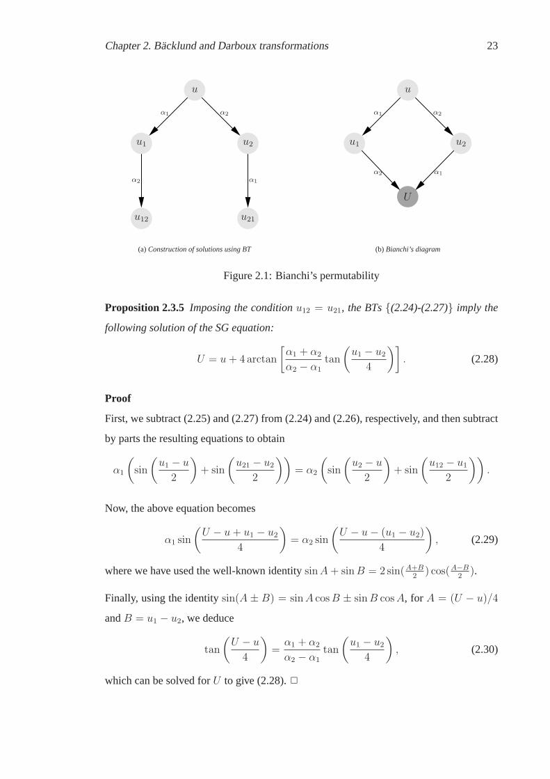
Proposition 2.3.5 Imposing the conditionu12 = u21, the BTs{(2.24)-(2.27)} imply the
following solution of the SG equation:
U = u+ 4arctan
[
α1 + α2
α2 − α1
tan
(
u1 − u24
)]
. (2.28)
Proof
First, we subtract (2.25) and (2.27) from (2.24) and (2.26),respectively, and then subtract
by parts the resulting equations to obtain
α1
(
sin
(
u1 − u
2
)
+ sin
(
u21 − u22
))
= α2
(
sin
(
u2 − u
2
)
+ sin
(
u12 − u12
))
.
Now, the above equation becomes
α1 sin
(
U − u+ u1 − u24
)
= α2 sin
(
U − u− (u1 − u2)
4
)
, (2.29)
where we have used the well-known identitysinA+ sinB = 2 sin(A+B2
) cos(A−B2
).
Finally, using the identitysin(A ± B) = sinA cosB ± sinB cosA, for A = (U − u)/4
andB = u1 − u2, we deduce
tan
(
U − u
4
)
=α1 + α2
α2 − α1
tan
(
u1 − u24
)
, (2.30)
which can be solved forU to give (2.28).✷

Chapter 2. Backlund and Darboux transformations 24
Remark 2.3.6 One can verify thatU given in (2.28) satisfies both equations (2.26) (where
U = u12) and (2.27) (whereU = u21) modulo equations (2.24) and (2.25). Moreover, it
satisfies the corresponding temporal part of equations (2.26) and (2.27).
Remark 2.3.7 Relation (2.28) is nothing else but a nonlinear superposition principle for
the production of solutions of the SG equation.
2.3.2 Backlund transformation for the PKdV equation
An auto-Backlund transformation associated to the PKdV equation is given by the
following relations
Bα :
(u+ v)x = 2α + 12(u− v)2,
(u− v)t = 3(u2x − v2x)− (u− v)xxx,
(2.31)
which was first presented in 1973 in a paper of Wahlquist and Estabrook [90]. In this
section we show how we can construct algebraically a solution of the PKdV equation,
using Bianchi’s permutability.
Bianchi’s permutability: Nonlinear superposition princip le of solutions of the PKdV
equation
Let u = u(x, t) be a function satisfying the PKdV equation. Focusing on the spatial part
of the BT (2.31), we can construct two new solutions, fromu1 = Bα1(u) andu2 = Bα2
(u),
i.e.
(u1 + u)x = 2α1 +1
2(u1 − u)
2, (2.32)
(u2 + u)x = 2α2 +1
2(u2 − u)
2. (2.33)
Moreover, following 2.1-(b), we can construct two more fromrelationsu12 = Bα2(u1)
andu21 = Bα1(u2), i.e.
(u12 + u1)x = 2α2 +1
2(u12 − u1)
2, (2.34)
(u21 + u2)x = 2α1 +1
2(u21 − u2)
2. (2.35)

Chapter 2. Backlund and Darboux transformations 25
Proposition 2.3.8 Imposing the conditionu12 = u21, the BTs{(2.32)-(2.35)} imply the
following solution of the PKdV equation:
U = u− 4α1 − α2
u1 − u2. (2.36)
Proof
It is straightforward calculation; one needs to subtract (2.33) and (2.35) by (2.32) and
(2.34), respectively, and subtract the resulting equations.✷
In the next chapter –where we study Darboux transformationsfor particular NLS type
equations– we shall see that BT arise naturally in the derivation of DT.
Chapter 2. Backlund and Darboux transformations 26

27
Chapter 3
Darboux tranformations for NLS type
equations and discrete integrable
systems
3.1 Overview
As we have seen in the previous chapter, Darboux and Backlund transformations are
closely related to the notion of integrability [80]. They can be derived from Lax pairs in a
systematic way, e.g. [20, 21], and provide the means to construct classes of solutions for
the integrable equations to which they are related. Moreover, they can be interpreted as
differential-difference equations [10, 56, 57, 67] and their commutativity, also referred to
as Bianchi’s permutability theorem, leads to systems of difference equations [7, 71, 78].
In this chapter we use Lax operators which are invariant under the action of the reduction
group to derive Darboux transformations. We interpret the associated Darboux matrices
as Lax matrices of a discrete Lax pair and construct systems of difference equations.
More precisely, our starting point is the general Lax operator
L = Dx + U(p, q;λ). (3.1)
Here, the2 × 2 matrix U belongs to the Lie algebrasl(2,C), depends implicitly onx

Chapter 3. Darboux tranformations for NLS type equations anddiscrete integrablesystems 28
through potentialsp, q, and depends rationally on the spectral parameterλ. Imposing
the invariance of operatorL under the action of the automorphisms ofsl(2,C), i.e. the
reduction group, inequivalent classes of Lax operators canbe constructed systematically.
This classification of the corresponding automorphic Lie algebras was presented in [60],
which were also derived in [16] in a different way.
Because of this construction, the resulting Lax operators have specificλ-dependence
and possess certain symmetries. We shall be assuming that the corresponding Darboux
transformations inherit the sameλ-dependence and symmetries, hence the derivation
of these transformations is considerably simplified in thiscontext. Once a Darboux
transformation has been derived, one may construct algorithmically new fundamental
solutions, i.e. solutions of the equationLΨ = 0, from a given initial one using
this transformation. Moreover, combining two different Darboux transformations and
imposing their commutativity, a set of algebraic relationsamong the potentials involved
in L results as a necessary condition.
One may interpret these potentials as functions defined on a two dimensional lattice
and, consequently, the corresponding algebraic relationsamong them as a system of
difference equations. One interesting characteristic of the resulting discrete systems is
their multidimensional consistency [8, 9, 15, 68, 69, 72]. This means that these systems
can be extended into a three dimensional lattice in a consistent way and, consequently, in
an infinite dimensional lattice.
Another property of these systems, following from their derivation, is that they admit
symmetries. The latter are nothing else but the Backlund transformation of the
corresponding continuous system to which the Lax operatorL is related.
The chapter is organised as follows: In the next section we briefly explain what is a
reduction group, what automorphic Lie algebras are and we list the cases of the PDEs we
study; the nonlinear Schrodinger equation, the derivative nonlinear Schrodinger equation
and a deformation of the derivative nonlinear Schrodinger equation. In section 3 we
present the general scheme we follow to derive Darboux matrices and construct systems
of difference equations. Finally, section 4 is devoted to the derivation of Darboux matrices
for NLS type equations, while section 5 deals with employingthese Darboux matrices to

Chapter 3. Darboux tranformations for NLS type equations anddiscrete integrablesystems 29
construct discrete integrable systems and their integrable reductions.
The results of this chapter appear in [50].
3.2 The reduction group and automorphic Lie algebras
The reduction group was first introduced in [63, 64]. It is a discrete group of
automorphisms of a Lax operator, and its elements are simultaneous automorphisms of the
corresponding Lie algebra and fractional-linear transformations of the spectral parameter.
Automorphic Lie algebras were introduced in [58, 59] and studied in [16, 17, 58, 59, 60].
These algebras constitute a subclass of infinite dimensional Lie algebras and their name
is due to their construction which is very similar to the one for automorphic functions.
Following Klein’s classification [48] of finite groups of fractional-linear transformations
of a complex variable, in [16, 17] it has been shown that in thecase of2 × 2 matrices,
which we study in this chapter, the essentially different reduction groups are
• the trivial group (with no reduction);
• the cyclic reduction groupZ2 (leading to the Kac-Moody algebraA11);
• the Klein reduction groupZ2 × Z2∼= D2.
Reduction groupsZ2 andD2 have bothdegenerateandgenericorbits. Degenerate are
those orbits that correspond to the fixed points of the fractional-linear transformations of
the spectral paramater, while the others are called generic.
Now, the following Lax operators
L = Dx + λ
1 0
0 −1
+
0 2p
2q 0
, (3.2a)
L = Dx + λ2
1 0
0 −1
+ λ
0 2p
2q 0
, (3.2b)
L = Dx + (λ2 − λ−2)
1 0
0 −1
+ λ
0 2 p
2 q 0
+ λ−1
0 2 q
2 p 0
, (3.2c)

Chapter 3. Darboux tranformations for NLS type equations anddiscrete integrablesystems 30
constitute all the essential different Lax operators, withpoles of minimal order, invariant
with respect to the generators ofZ2 andD2 groups with degenerate orbits. In what follows,
we study the Darboux transformations for all the above cases.
Operator (3.2a) is associated with the NLS equation [93],
pt = pxx + 4p2q, qt = −qxx − 4pq2, (3.3)
while (3.2b) and (3.2c) are associated with the DNLS equation [47],
pt = pxx + 4(p2q)x, qt = −qxx + 4(pq2)x. (3.4)
and a deformation of the DNLS equation [65]
pt = pxx + 8(p2q)x − 4qx, qt = −qxx + 8(pq2)x − 4px, (3.5)
respectively.
3.3 General framework
In this section we present the general framework for the derivation of Darboux matrices
related to Lax operators of AKNS type. Moreover, we explain how we can employ these
Darboux matrices to construct discrete integrable systems.
3.3.1 Derivation of Darboux matrices
The Lax operators which we consider in the rest of this thesisare of the following AKNS
form
L(p, q;λ) = Dx + U(p, q;λ), (3.6)
whereU is a2 × 2 traceless matrix which belongs in the Lie algebrasl(2,C), depends
implicitly on x through the potential functionsp andq and is a rational function in the
Chapter 3. Darboux tranformations for NLS type equations anddiscrete integrablesystems 31
spectral parameterλ ∈ C. We also require that the dependence on the spectral parameter
is nontrivial1.
Remark 3.3.1 In the forthcoming analysis we shall only be needing the spatial part of
the Lax pair of the associated PDEs.
In what follows, by Darboux transformation we understand a map
L → L =MLM−1, (3.7)
whereL has exactly the same form asL but updated with new potentialsp10 andq10,
namely
L = Dx + U(p10, q10;λ). (3.8)
Matrix M in (3.7) is an invertible matrix called theDarboux matrix.
According to definition (3.7), a Darboux matrix may depend onany of the potential
functionsp, q, p10 andq10, and the spectral parameterλ. Moreover, given a Lax operator
L, we can calculate the Darboux matrix using the following.
Proposition 3.3.2 Given a Lax operator of the form (3.6), the Darboux matrix,M ,
satisfies the following equation
DxM + U10M −MU = 0, (3.9)
whereU10 = U(p10, q10;λ).
Proof
By definition of the Darboux transformation we have thatLM =ML, namely
(Dx + U(p10, q10;λ))M =M(Dx + U(p, q;λ)). (3.10)
1By nontrivial we mean thatλ cannot be eliminated by a gauge transformation. For instance, matrix
∗ λ−1
∗
has trivial dependence onλ since
λ1/2
λ−1/2
∗ λ−1
∗
λ1/2
λ−1/2
−1
=
∗ 1
∗
Chapter 3. Darboux tranformations for NLS type equations anddiscrete integrablesystems 32
Therefore, sinceDx ·M = Mx +MDx, the above equation implies thatM must obey
equation (3.9).✷
Although the above proposition can be used to determineM , this cannot be done in full
generality without making choices forM and analysing its dependence on the spectral
parameterλ.
Our first choice will be based on the following.
Proposition 3.3.3 A composition of two Darboux matrices for an operator of the form
(3.6) is a Darboux matrix for the same operator.
Proof
LetM andK be Darboux matrices for an operatorL of the form (3.6). Then,
LM =ML, LK = KL. (3.11)
by definition of the Darboux matrix. Now,
KML(3.11)= KLM
(3.11)= ˆLKM. (3.12)
Therefore,ˆL = KML(KM)−1 which proves the statement.✷
We define therank of a Darboux transformation to be the rank of the matrix which
appears as coefficient of the higher power of the spectral parameter. In the next sections,
we shall be assuming that the Darboux tranformations are of rank 1; in fact, in some
examples, Darboux transformations of full rank can be written as composition of Darboux
transformations of rank 1.
The second choice is related to the form of the correspondingLax operators. Since the Lax
operators we deal with have rational dependence on the spectral parameter, we impose
without loss of generality, that the same holds for matrixM as well. Moreover, we employ
any symmetries of the Lax operator,L, as symmetries inherited toM . Specifically, if the
Chapter 3. Darboux tranformations for NLS type equations anddiscrete integrablesystems 33
the Lax operator2 L(λ) satisfies a relation of the form
L(λ) = Σ(λ)L(σ(λ))Σ(λ)−1, (3.13)
for some invertible functionσ(λ) and some invertible matrixΣ(λ), then we shall be
assuming thatM must obey the same relation, namely
M(λ) = Σ(λ)M(σ(λ))Σ(λ)−1. (3.14)
Relation (3.14) imposes some restrictions on the form of matrix M and reduces the
number of functions involved in it.
Now, letM be a Darboux matrix for the operatorL, andΨ = Ψ(x, λ) a fundamental
solution of the linear equation
LΨ(x, λ) = 0. (3.15)
Then, we have the following.
Proposition 3.3.4 Matrix M maps fundamental solutions of (3.15) to fundamental
solutions ofLΨ = 0. Moreover, the determinant ofM is independent ofx.
Proof
LetM mapΨ toΨ10, namelyΨ10 =MΨ. Then, according to (3.7)
LΨ10 =MLM−1Ψ10 =MLM−1(MΨ) =MLΨ = 0, (3.16)
i.e. Ψ10 is a solution ofLΨ = 0. Moreover,Ψ10 is fundamental, sinceΨ is fundamental,
detM 6= 0 andΨ10 =MΨ.
Now, recall Liouville’s formula3 for solutions of the linear equationLΨ = 0, given by
detΨ(x, t;λ) = detΨ(x0, t;λ) exp
(
−
∫ x
x0
trU(p(ξ), q(ξ);λ)dξ
)
. (3.17)
SinceU is traceless, from the above formula we deduce that the determinants ofΨ and
Ψ10 are non-zero and independent ofx. Hence, the relationΨ10 = MΨ implies that
∂x(det(M)) = 0. ✷
2For simplicity of the notation, we sometimes omit the dependence on the potentialsp and q, i.e.
L(p, q;λ) ≡ L(λ).3It is also known as Abel-Jacobi-Liouville identity.

Chapter 3. Darboux tranformations for NLS type equations anddiscrete integrablesystems 34
3.3.2 Discrete Lax pairs and discrete systems
Starting with a fundamental solution of equation (3.15), say Ψ, we can employ two
Darboux matrices to derive two new fundamental solutionsΨ10 andΨ01 as follows
Ψ10 =M(p, q, p10, q10;λ)Ψ ≡MΨ, Ψ01 =M(p, q, p01, q01;λ)Ψ ≡ KΨ. (3.18)
Then, a third solution can be derived in a purely algebraic way as shown in Figure 3.1.
Ψ Ψ10M
Ψ01 Ψ11M01
K K10
Figure 3.1: Bianchi commuting diagram
Specifically, starting with two fundamental solutions of equation (3.15),Ψ10 andΨ01, one
can construct two new fundamental solutions using Darboux matrices
M(p10, q10, p11, q11;λ) ≡ K10 M(p01, q01, p11, q11;λ) ≡M01,
namely the following
X :=M01Ψ01 =M01KΨ ≡M(p01, q01, p11, q11;λ)M(p, q, p01, q01;λ)Ψ,
Y := K10Ψ10 = K10MΨ ≡M(p10, q10, p11, q11;λ)M(p, q, p10, q10;λ)Ψ.
Imposing that these two different solutions coincide, i.e.X = Y = Ψ11 (see Figure 3.1),
the following condition must hold
M01K −K10M = 0. (3.19)
If the latter condition is written out explicitly, it results in algebraic relations among the
various potentials involved.
We can interpret the above construction in a discrete way. Particularly, let us assume that
p andq are functions depending not only onx but also on two discrete variablesn andm,

Chapter 3. Darboux tranformations for NLS type equations anddiscrete integrablesystems 35
i.e. p = p(x;n,m) andq = q(x;n,m). Furthermore, we define theshift operatorsS and
T acting on a functionf = f(n,m) as
Sf(n,m) = f(n+ 1,m), T f(n,m) = f(n,m+ 1). (3.20)
We shall refer toS andT as theshift operators in then and them-direction, respectively.
Now, we expect that the shift operatorsS andT commute with each other and with the
differential operator∂x. In particular, we have the following.
Proposition 3.3.5 The shift operatorsS andT commute with each other and also with
the partial differential operator on solutions ofLΨ = 0.
Proof
LetΨ be a solution ofLΨ = 0. For the commutativity ofS andT we have that
T SΨ = T (MΨ) =M01Ψ01 =M01KΨ, (3.21)
and on the other hand
ST Ψ = S(KΨ) = K10Ψ10 = K10MΨ, (3.22)
which proves that[S, T ] Ψ = 0, due to (3.19).
Now, we prove the commutativity between the shift operatorS and the partial differential
operator, and the proof is exactly the same forT . We basically need to show thatSΨx =
(SΨ)x. Indeed,
(SΨ)x = ∂xΨ10(3.18)= (MΨ)x =MxΨ+MΨx
(3.6)= MxΨ−MUΨ. (3.23)
On the other hand, we have that
SΨx
(3.6)= −S(UΨ) = −U10Ψ10
(3.18)= −U10MΨ. (3.24)
Due to proposition 3.3.2, the right hand sides of (3.24) and (3.23) are equal which
completes the proof.✷
Chapter 3. Darboux tranformations for NLS type equations anddiscrete integrablesystems 36
In addition, we interpret the shifts ofp andq with
pij = p(x;n+ i,m+ j), qij = q(x;n+ i,m+ j), p00 ≡ p, q00 ≡ q, (3.25)
respectively.
In this notation, system (3.18) can be considered as a discrete Lax pair, and equation
(3.19) is nothing but its compatibility condition. Furthermore, the resulting polynomials
from condition (3.19) define a system of partial difference equations forp andq.
Note 3.3.6 For the sake of simplicity, in the rest of the thesis, we adoptthe following
notation: the derivative with respect tox of a scalar object with lower indices, say∂xpij,
will be denoted bypij,x. Moreover, for a matrix with lower index, sayM0, with M0,ij we
shall denote its(i, j)-element.
Now let u be a solution of a system of difference equations,∆(u) = 0. Moreover, letu
be given by
u := Rǫ(u) = u + ǫ r(u), (3.26)
wereǫ is an infinitesimal parameter. We have the following ([66]).
Definition 3.3.7 We shall say thatRǫ(u) constitutes an infinitensimal symmetry –or just
a symmetry– of∆(u) = 0, if u := Rǫ(u) is also a solution up to orderǫ2, namely
∆(u) = O(ǫ2). (3.27)
Corollary 3.3.8 Map Rǫ(u) defined in (3.26) is a symmetry of a system of difference
equations,∆(u), if the following condition4
∑
i,j∈Z
∂∆
∂uij
S iT jr(u) = 0, (3.28)
is satisfied mod 〈∆(u) = 0〉.
4OperatorD∆ :=∑
i,j∈Z
∂∆∂uijSiT j is called theFrechet derivative.

Chapter 3. Darboux tranformations for NLS type equations anddiscrete integrablesystems 37
Proof
If we expand∆(u + ǫr(u)) in series, then equating theǫ-terms, (3.27) implies (3.28).✷
In the next section we shall see for particular examples that, the derivation of Darboux
matrices gives rise to particular differential-difference equations which possess first
integrals. In some cases, the latter may be used to reduce thenumber of the dependent
variables and derive scalar equations; some of them are of Toda type and some others are
defined on a stencil of six or seven points. Additionally, theform of these systems allows
us to pose an initial value problem on the staircase.
The derived system of differential-difference equations is, in general, of the form
P(p, q, ∂xp, ∂xq, ∂xp10, ∂xq10) = 0. (3.29)
However, in all the examples of this thesis, system (3.29) boils down to an evolutionary
differential-difference system of equations of the form
px = Z(p, p10), p = (p, q), (3.30)
and its shifted consequences.
For the above system of equations we have the following.
Proposition 3.3.9 The differential-difference equations (3.30) constitutegenerators of
generalised symmetries of the associated system of difference equations.
Proof
Indeed,
d
dx(M01K −K10M) =M01,xK +M01Kx −K10,xM −K10Mx. (3.31)
Now, according to Proposition 3.3.2 we have
Mx =MU − U10M, M01,x =M01U01 − U11M01
Kx = KU − U01K, K10,x = K10U10 − U11K10.
Chapter 3. Darboux tranformations for NLS type equations anddiscrete integrablesystems 38
Therefore,
d
dx(M01K −K10M) = U11(K10M −M01K) + (M01K −K10M)U. (3.32)
The right-hand-side of the above is zeromod 〈K10M −M01K = 0〉 which proves the
statement.✷
Note 3.3.10System (3.30) is nothing but thex-part (spatial-part) of a Backlund transfo-
rmation between solutions of the PDE associated to the Lax operator.
In the next section we derive Darboux matrices for particular PDEs of NLS type; the NLS
equation, the DNLS equation and a deformation of the DNLS equation.
In all the above cases, we find more than one Darboux matrix. Atthis point it is worth
mentioning that, the interpretation of any pair of Darboux matrices as a discrete Lax pair
does not always lead to a discrete integrable system. On the contrary, in several cases, the
compatibility condition (3.19) yields a trivial system.
3.4 NLS type equations
In this section we study the Darboux transformations related to the NLS type equations
discussed earlier.
As an illustrative example, we start with the NLS equation.
3.4.1 The nonlinear Schrodinger equation
The Lax operator in this case is given by
L := Dx + U(p, q;λ) = Dx + λU1 + U0, (3.33a)
whereU1 andU0 are given by
U1 ≡ σ3 = diag(1,−1), U0 =
0 2p
2q 0
. (3.33b)

Chapter 3. Darboux tranformations for NLS type equations anddiscrete integrablesystems 39
OperatorL is the spatial part of the Lax pair for the nonlinear Schrodinger equation.
The NLS equation has the following scaling symmetry
p10 = αβ−1p, q10 = βα−1q. (3.34)
A spectral parameter independent Darboux matrix corresponding to the above symmetry
is given by the following constant matrix
M =
α 0
0 β
, αβ 6= 0. (3.35)
Now, we seek Darboux matrices which depend on the spectral parameter,λ. The simplest
λ-dependence is a linear dependence. In particular, we have the following.
Proposition 3.4.1 LetM be a Darboux matrix for the Lax operator (3.33) and suppose
it is linear in λ. Let alsoM define a Darboux transformation of rank 1. Then, up to a
gauge transformation,M is given by
M(p, q10, f) := λ
1 0
0 0
+
f p
q10 1
, (3.36)
where the potentialsp andq satisfy the following differential-difference equations
∂xf = 2(pq − p10q10), (3.37a)
∂xp = 2(pf − p10), (3.37b)
∂xq10 = 2(q − q10f). (3.37c)
Moreover, matrix (3.36) degenerates to
Mc(p, f) = λ
1 0
0 0
+
f p
cp
0
, f =px2p. (3.38)
Proof
Let us suppose thatM is of the formM = λM1+M0. Substitution ofM to equation (3.9)
implies a second order algebraic equation inλ. Equating the coefficients of the several

Chapter 3. Darboux tranformations for NLS type equations anddiscrete integrablesystems 40
powers ofλ equal to zero, we obtain the following system of equations
λ2 : [σ3,M1] = 0, (3.39a)
λ1 : M1,x + [σ3,M0] + U010M1 −M1U
0 = 0, (3.39b)
λ0 : M0,x + U010M0 −M0U
0 = 0, (3.39c)
where with[σ3,M1] we denote the commutator ofσ3 andM1.
Equation (3.39a) implies thatM1 must be diagonal, i.e.M1 = diag(c1, c2). Then, we
substituteM1 to (3.39b).
Now, for simplicity of the notation, we denote the(1, 1) and(2, 2) entries ofM0 by f and
g respectively. Then, it follows from equation (3.39c) that the entries of matrixM0 must
satisfy the following equations
∂xf = 2(M0,12q − p10M0,21), (3.40a)
∂xg = 2(M0,21p− q10M0,12), (3.40b)
∂xM0,12 = 2(pf − gp10), (3.40c)
∂xM0,21 = 2(qg − q10f). (3.40d)
The off-diagonal part of (3.39b) implies that the(1, 2) and(2, 1) entries of matrixM0 are
given by
M0,12 = c1p− c2p10, M0,21 = c1q10 − c2q. (3.41)
Additionally, from the diagonal part of (3.39b) we deduce that c1,x = c2,x = 0. Since
the Darboux transformation is of rank one, namelyrankM1 = 1, one of the constantsci,
i = 1, 2 must be zero. Thus, after rescaling we can choose eitherc1 = 1, c2 = 0 or c1 = 0,
c2 = −1. These two choices correspond to gauge equivalent Darboux matrices.
Indeed, the choicec1 = 1, c2 = 0 impliesM0,12 = p andM0,21 = q10. Moreover, (3.40b)
implies thatg = const.= α, i.e.
M0 =
f p
q10 α
. (3.42)
In this case the Darboux matrix is given by
λ
1 0
0 0
+
f p
q10 α
, (3.43)

Chapter 3. Darboux tranformations for NLS type equations anddiscrete integrablesystems 41
where, according to (3.40), its entries satisfy
∂xf = 2(pq − p10q10), ∂xp = 2(pf − αp10), ∂xq10 = 2(cq − q10f). (3.44)
Now, if α 6= 0, it can be rescaled toα = 1 and thus the Darboux matrix in this case is
given by (3.36) where its entries obey (3.37).
Similarly, the second choice,c1 = 0, c2 = −1, leads to the following Darboux matrix
N(p10, q, g) = λ
0 0
0 −1
+
1 p10
q g
. (3.45)
The above is gauge equivalent to (3.36), sinceσ1N(p10, q, g)σ−11 is of the form (3.36).
Therefore, a linear inλ Darboux matrix is given by (3.36) where its entries obey the
differential-difference equations (3.37).
In the case whereα = 0, from (3.44) we deduce
px = 2fp, q10,x = −2fq10. (3.46)
Thus, the Darboux matrix in this case is given by
M(p, q10, f) := λ
1 0
0 0
+
f p
q10 0
. (3.47)
In addition, after an integration with respect tox, equations (3.46) imply thatq10 = c/p.
Hence, the Darboux matrix in this case is given by (3.38).✷
It is straightforward to show that system (3.37) admits the following first integral
∂x (f − p q10) = 0 . (3.48)
which implies that∂x detM = 0.
3.4.2 The derivative nonlinear Schrodinger equation: Z2-reduction
group
The Lax operator in this case is given by
L = Dx + λ2U2 + λU1, (3.49a)

Chapter 3. Darboux tranformations for NLS type equations anddiscrete integrablesystems 42
where
U2 = σ3 =diag(1,−1) and U1 =
0 2p
2q 0
. (3.49b)
This is the spatial part of the Lax pair for the DNLS equation (3.4) , and it is invariant
under the transformation
s1(λ) : L(λ)→ σ3L(−λ)σ3. (3.50)
As a matter of fact, the above involution generates the reduction group which is
isomorphic to theZ2 group.
As in the case of the NLS equation, the DNLS equation has the following scaling
symmetry
p10 = αβ−1p, q10 = βα−1q. (3.51)
A spectral parameter independent Darboux matrix corresponding to the above symmetry
is given by the following constant matrix
M =
α 0
0 β
, αβ 6= 0. (3.52)
Now, we seek Darboux matrices with the sameλ-dependence as the non-differential part
of (3.49), namely of the form
M = λ2M2 + λM1 +M0. (3.53)
Lemma 3.4.2 A second order matrix polynomial inλ, of the form (3.53), is invariant
under the involution (3.50), iffM2 andM0 are diagonal matrices andM1 is off-diagonal.
Proof
It is straightforward if we demand thatM satisfies the condition:M(λ) = σ3M(−λ)σ3.
✷
As mentioned earlier, we shall restrict ourselves to Darboux transformations of rank 1,
and we have the following.

Chapter 3. Darboux tranformations for NLS type equations anddiscrete integrablesystems 43
Proposition 3.4.3 Let M in (3.53) be a Darboux matrix for the Lax operator (3.49)
that is invariant under the involution (3.50) andrankM2 = 1. Then, up to a gauge
transformation,M is given by
M(p, q10, f ; c1, c2) := λ2
f 0
0 0
+ λ
0 fp
fq10 0
+
c1 0
0 c2
, (3.54)
wherep andq satisfy the following differential-difference equations
∂xf = 2f (pq − p10q10) , (3.55a)
∂xp = 2p (p10q10 − pq)− 2c2p10 − c1p
f, (3.55b)
∂xq10 = 2q10 (p10q10 − pq)− 2c1q10 − c2q
f. (3.55c)
Proof
According to Lemma (3.4.2), matrixM2 should be diagonal. Additionally, since
rankM2 = 1, we considerM2 to be of the formM2 = diag(f, 0). The choise
M2 = diag(0, g) leads to a gauge equivalent Darboux transformation.
Now, 3.9 implies thatM satisfies the following system of equations
λ4 : [σ3,M2] = 0, (3.56a)
λ3 : [σ3,M1] + U110M2 −M2U
1 = 0, (3.56b)
λ2 : M2,x + [σ3,M0] + U110M1 −M1U
1 = 0, (3.56c)
λ1 : M1,x + U110M0 −M0U
1 = 0, (3.56d)
λ0 : M0,x = 0. (3.56e)
The first one, (3.56a), is satisfied automatically sinceM2 is diagonal. Moreover, the last
one, (3.56e), implies thatM0 is constant, i.e.M0 = diag(c1, c2), wherec1, c2 ∈ C.
From equation (3.56b) we determine the entries of the off-diagonal matrixM1, namely
M1,12 = fp and M1,21 = fq10. (3.57)
That is,M is given by (3.54).
Equation (3.56c) implies the first differential-difference equation (3.55a), while equation
(3.56d) implies the following
(fp)x = 2c1p− 2c2p10 and (fq10)x = 2c2q − 2c1q10. (3.58)

Chapter 3. Darboux tranformations for NLS type equations anddiscrete integrablesystems 44
With use of (3.55a), the above equations can be rewritten in the form (3.55b) and (3.55c),
respectively.✷
A first integral of the differential-difference equations (3.55) is given by
∂x(
f 2pq10 − c2f)
= 0. (3.59)
The above integral guarantees that the determinant of the Darboux matrix (3.54) is
independent ofx.
Remark 3.4.4 If the constantsc1 andc2 in (3.54) are non-zero, then we can rescale them
to 1, by composing with a Darboux matrix (3.52) and changingf → fα−1 andq10 →
q10αβ−1.
However, if either ofc1 or c2 is zero, we can bring the differential-difference equations
(3.55) into polynomial form.
Case I: c1 = c2 = 0. Modified Volterra chain
In this case, from equations (3.58), we obtain(fp)x = (fq10)x = 0. An integration of the
latter implies thatf = 1/p andq10 = p, where we have set the constants of integration
equal to 1. Hence, the Darboux matrix (3.54) degenerates to
Mdeg(p) := λ2
1/p 0
0 0
+ λ
0 1
1 0
. (3.60)
Moreover, the corresponding differential-difference equations become
q10 = p ∂xp = 2p2 (p10 − p−10) , (3.61)
and the first integral (3.59) holds identically. The resulting differential-difference
equations (3.61) constitute the modified Volterra chain [91].

Chapter 3. Darboux tranformations for NLS type equations anddiscrete integrablesystems 45
Case II: c1 = 1 and c2 = 0
In this case the Darboux matrix simplifies to
M(p, q10, f) := λ2
f 0
0 0
+ λ
0 fp
fq10 0
+
1 0
0 0
. (3.62)
The differential-difference equations (3.55) become
∂xf = 2f(pq − p10q10), (3.63a)
∂xp = 2p (p10q10 − pq) +2p
f, (3.63b)
∂xq10 = 2q10 (p10q10 − pq)−2q10f, (3.63c)
and the first integral (3.59) can be rewritten as
∂x(
f 2pq10)
= 0. (3.64)
Now, in order to expressf in terms ofp andq, avoiding any square roots, we make the
following point transformation
p = u2, q = v2−10. (3.65)
Thus, the first integral (3.64) impliesf 2u2v2 = 1 and, subsequently,f is given byf =
±1/uv. Moreover, for thisf , system (3.63) can be rewritten in a polynomial form as
∂xu = u(u210v2 − u2v2−10)± u
2v, ∂xv = v(u210v2 − u2v2−10)∓ uv
2. (3.66)
3.4.3 A deformation of the derivative nonlinear Schrodinger equa-
tion: Dihedral reduction group
In this case, the Lax operator5 is given by
L = Dx + λ2U2 + λU1 + λ−1U−1 + λ−2U−2, (3.67a)
5The full Lax pair of the associated PDE can be found in [16, 17].

Chapter 3. Darboux tranformations for NLS type equations anddiscrete integrablesystems 46
where
U2 ≡ −U−2 = σ3, U1 ≡ (U−1)T =
0 2 p
2 q 0
. (3.67b)
Operator (3.67) is the spatial part of the Lax pair of the deformation of the DNLS equation
(3.5) , and it is invariant under the following transformations
s1(λ) : L(λ)→ σ3L(−λ)σ3, (3.68a)
s2(λ) : L(λ)→ σ1L(1
λ)σ1, σ1 =
0 1
1 0
. (3.68b)
The above involutions generate the reduction group which isisomorphic toZ2×Z2∼= D2
(dihedral group).
Equation (3.5) has the obvious symmetry(p, q) → (−p,−q). A spectral parameter
independent Darboux matrix for (3.67), which corresponds to the latter symmetry, is given
by σ3. For aλ-dependent Darboux matrix, we seek a matrix with the same dependence
on the spectral parameter as the non-differential part ofL in (3.67). Specifically, we are
seeking forM of the form
M = λ2M2 + λM +M0 + λ−1M−1 + λ−2M−2. (3.69)
Lemma 3.4.5 A matrix of the form (3.69), which is invariant under the involutionss1 and
s2 in (3.68), is given by
M = λ2
α 0
0 β
+ λ
0 γ
δ 0
+
µ 0
0 ν
+ λ−1
0 δ
γ 0
+ λ−2
β 0
0 α
.
Proof
RelationM(λ) = σ3M(−λ)σ3 implies thatM0, M2 andM−2 must be diagonal, whereas
M1 andM−1 must be off-diagonal. Moreover, from relationM(λ) = σ1M(1/λ)σ1, we
obtain:M2,11 =M−2,22,M2,22 =M−2,11,M1,12 =M1,21 andM1,21 =M1,12. ✷

Chapter 3. Darboux tranformations for NLS type equations anddiscrete integrablesystems 47
Proposition 3.4.6 LetM be a Darboux matrix of the form (3.69) for the Lax operator
(3.67) andrankM2 = 1. Moreover, suppose that it is invariant under the involutionss1
ands2. Then, up to a gauge transformation and an additive constant,M is given by
M(p, q10, f, g) := f
λ2 0
0 λ−2
+ λ
0 p
q10 0
+ gI + λ−1
0 q10
p 0
(3.70)
whereI is the identity matrix andp, q, f andg satisfy the following system of differential-
difference equations
∂xp = 2(
(p10q10 − pq)p+ (p− p10)g + q − q10
)
, (3.71a)
∂xq10 = 2(
(p10q10 − pq)q10 + (q − q10)g + p− p10
)
, (3.71b)
∂xg = 2(
(p10q10 − pq)g + (p− p10)p+ (q − q10)q10
)
, (3.71c)
∂xf = 2(pq − p10q10)f. (3.71d)
Proof
From equation (3.9) we deduce the system of equations
λ4 : [σ3,M2] = 0, (3.72a)
λ3 : [σ3,M1] + U110M2 −M2U
1 = 0, (3.72b)
λ2 : M2,x + U110M1 −M1U
1 = 0, (3.72c)
λ1 : M1,x + [σ3,M−1] + U110M0 −M0U
1 + U−110 M2 −M2U
−1 = 0, (3.72d)
λ0 : M0,x + U110M1 −M−1U
1 + U−110 M1 −M1U
−1 = 0, (3.72e)
for the entries ofM . Because of the symmetry, the negative powers ofλ correspond to
the same equations as the above.
Equation (3.72a) is automatically satisfied asM2 is diagonal. From equation (3.72b) we
identify the entriesγ andδ of matrixM1 in terms of the potentials, namely
γ = αp− βp10 and δ = αq10 − βq, (3.73)
whereas from (3.72d) we can express their derivatives in terms of the potentials and the
entries of matricesM2 andM0 as
γx = 2 (αq − βq10 + µp− νp10 − δ) , (3.74a)
δx = 2 (βp− αp10 + νq − µq10 + γ) . (3.74b)

Chapter 3. Darboux tranformations for NLS type equations anddiscrete integrablesystems 48
Now, from equation (3.72c) we obtain the derivatives ofα andβ in terms of the potentials,
γ andδ, namely
αx = 2(γq − δp10) and βx = 2(δp− γq10). (3.75)
Substituting (3.73) into the above equations, we deduce that αβ =const. Moreover, since
rankM2 = 1, eitherα or β has to be zero. Thus, we can chooseβ = 0 and, then,α can
be any arbitrary function ofx, sayα = f(x). The caseα = 0 andβ = f(x) leads to a
Darboux matrix which is gauge equivalent to the former.
Now,α = f(x) andβ = 0 imply thatγ = fp andδ = fq10 from (3.73).
The last equation of (3.72) implies
µx = νx = 2f (p(p− p10) + q(q − q10)) . (3.76)
Therefore, after a simple integration, we deduce thatµ = ν (where we have assumed that
the integration constant is zero).
Now, the first equation of (3.75) can be rewritten as
fx = 2f(pq − p10q10). (3.77)
Using the above, and since we have expressedγ andδ in terms off , p andq10, equations
(3.74) can be rewritten as
px = 2(
(p10q10 − pq)p+ q − q10 +µ
f(p− p10)
)
, (3.78a)
q10,x = 2(
(p10q10 − pq)q10 + p− p10 +µ
f(q − q10)
)
. (3.78b)
Now, without any loss of generality, we can set6 µ = fg, which proves the statement.✷
It is straightforward to show that the quantities
Φ1 := f 2 (g − pq10) , Φ2 := f 2(
g2 + 1− p2 − q210)
, (3.79)
are first integrals for the system of equations (3.71), namely ∂xΦi = 0, i = 1, 2. In fact,
these first integrals imply that matrixM has constant determinant, since
detM =(
λ2 + λ−2)
Φ1 + Φ2. (3.80)
6This choice was made in order to retrieve polynomial expressions in (3.78).
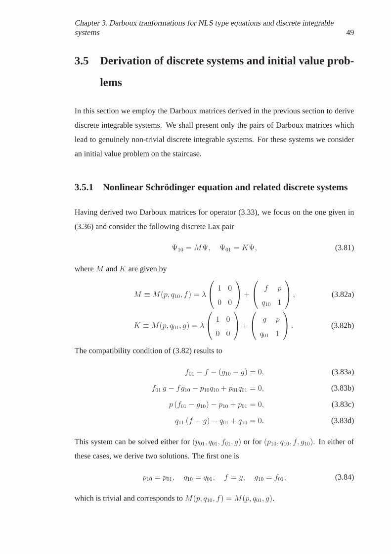
Chapter 3. Darboux tranformations for NLS type equations anddiscrete integrablesystems 49
3.5 Derivation of discrete systems and initial value prob-
lems
In this section we employ the Darboux matrices derived in theprevious section to derive
discrete integrable systems. We shall present only the pairs of Darboux matrices which
lead to genuinely non-trivial discrete integrable systems. For these systems we consider
an initial value problem on the staircase.
3.5.1 Nonlinear Schrodinger equation and related discrete systems
Having derived two Darboux matrices for operator (3.33), wefocus on the one given in
(3.36) and consider the following discrete Lax pair
Ψ10 =MΨ, Ψ01 = KΨ, (3.81)
whereM andK are given by
M ≡M(p, q10, f) = λ
1 0
0 0
+
f p
q10 1
, (3.82a)
K ≡M(p, q01, g) = λ
1 0
0 0
+
g p
q01 1
. (3.82b)
The compatibility condition of (3.82) results to
f01 − f − (g10 − g) = 0, (3.83a)
f01 g − fg10 − p10q10 + p01q01 = 0, (3.83b)
p (f01 − g10)− p10 + p01 = 0, (3.83c)
q11 (f − g)− q01 + q10 = 0. (3.83d)
This system can be solved either for(p01, q01, f01, g) or for (p10, q10, f, g10). In either of
these cases, we derive two solutions. The first one is
p10 = p01, q10 = q01, f = g, g10 = f01, (3.84)
which is trivial and corresponds toM(p, q10, f) =M(p, q01, g).

Chapter 3. Darboux tranformations for NLS type equations anddiscrete integrablesystems 50
The second solution is given by
p01 =q10p
2 + (g10 − f)p+ p101 + pq11
, q01 =p10q11
2 + (f − g10)q11 + q101 + pq11
, (3.85a)
f01 =q11(p10 + pg10) + f − pq10
1 + pq11, g =
q11(pf − p10) + g10 + pq101 + pq11
. (3.85b)
The above system has some properties which take their rise inthe derivation of the
Darboux matrix. In particular, we have the following.
Proposition 3.5.1 System (3.85) admits two first integrals,F := f − pq10 and G :=
g − pq01, and the following conservation law
(T − 1)f = (S − 1)g (3.86)
Proof
Relation (3.48) suggests that
(T − 1) (f − pq10) = 0 and (S − 1) (g − pq01) = 0, (3.87)
which can be verified with straightforward calculation, using equations (3.83a). Thus,
F = f − pq10 andG := g − pq01 are first integrals. Moreover, equation (3.83a) can be
written in the form of the conservation law (3.86).✷
Corollary 3.5.2 The following relations hold.
f − pq10 = α(n) and g − pq01 = β(m). (3.88)
Remark 3.5.3 In view of relations (3.88), we can interpret functionsf andg as being
given on the edges of the quadrilateral where system (3.85) is defined, and, consequently,
consider system (3.85) as a vertex-bond system [42].
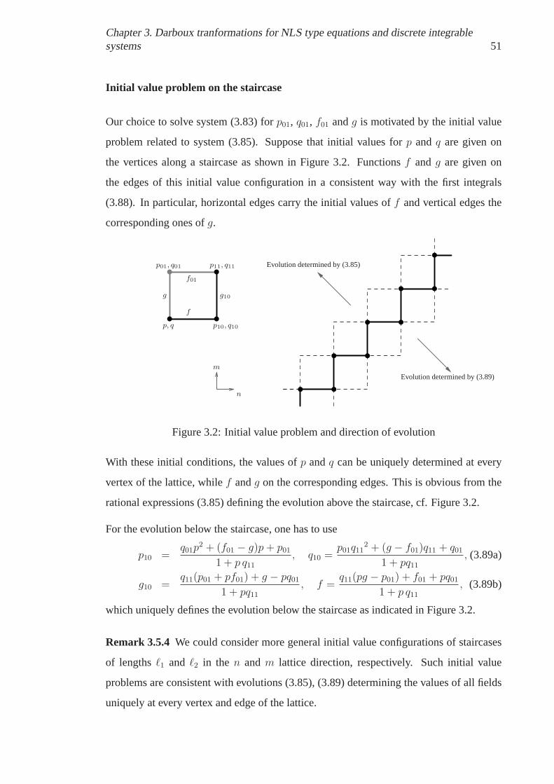
Chapter 3. Darboux tranformations for NLS type equations anddiscrete integrablesystems 51
Initial value problem on the staircase
Our choice to solve system (3.83) forp01, q01, f01 andg is motivated by the initial value
problem related to system (3.85). Suppose that initial values forp andq are given on
the vertices along a staircase as shown in Figure 3.2. Functionsf andg are given on
the edges of this initial value configuration in a consistentway with the first integrals
(3.88). In particular, horizontal edges carry the initial values off and vertical edges the
corresponding ones ofg.
g g10
n
m
p, q p10, q10
f
f01
p01, q01 p11, q11 Evolution determined by (3.85)
Evolution determined by (3.89)
Figure 3.2: Initial value problem and direction of evolution
With these initial conditions, the values ofp andq can be uniquely determined at every
vertex of the lattice, whilef andg on the corresponding edges. This is obvious from the
rational expressions (3.85) defining the evolution above the staircase, cf. Figure 3.2.
For the evolution below the staircase, one has to use
p10 =q01p
2 + (f01 − g)p+ p011 + p q11
, q10 =p01q11
2 + (g − f01)q11 + q011 + pq11
, (3.89a)
g10 =q11(p01 + pf01) + g − pq01
1 + pq11, f =
q11(pg − p01) + f01 + pq011 + p q11
, (3.89b)
which uniquely defines the evolution below the staircase as indicated in Figure 3.2.
Remark 3.5.4 We could consider more general initial value configurationsof staircases
of lengthsℓ1 and ℓ2 in the n andm lattice direction, respectively. Such initial value
problems are consistent with evolutions (3.85), (3.89) determining the values of all fields
uniquely at every vertex and edge of the lattice.

Chapter 3. Darboux tranformations for NLS type equations anddiscrete integrablesystems 52
Derivation of an Adler-Yamilov type of system
Now, using first integrals we can reduce system (3.85) to anAdler-Yamilov typeof system
as those in [10]. Specifically, we have the following.
Proposition 3.5.5 System (3.85) can be reduced to the following non-autonomousAdler-
Yamilov type of system forp andq:
p01 = p10 −α(n)− β(m)
1 + pq11p, q01 = q10 +
α(n)− β(m)
1 + pq11q11. (3.90)
Proof
The proof is straightforward if one uses relations (3.88) toreplacef and g in system
(3.85).✷
Derivation of discrete Toda equation
Now, we will use two different Darboux matrices associated with the NLS equation to
construct the discrete Toda equation [82].
In fact, we introduce a discrete Lax pair as (3.81), withM = M1(p, f) in (3.38) and
K =M(p, q01, g) in (3.36). That is, we consider the following system
Ψ10 =
λ
1 0
0 0
+
f p
1p
0
Ψ, (3.91a)
Ψ01 =
λ
1 0
0 0
+
g p
q01 1
Ψ, (3.91b)
and impose its compatibility condition.
From the coefficient of theλ-term in the latter condition we extract the following
equations
f − f01 = g − g10, (3.92a)
p01 =1
q11. (3.92b)

Chapter 3. Darboux tranformations for NLS type equations anddiscrete integrablesystems 53
Additionally, theλ0-term of the compatibility condition implies
f01g − g10f =p10p− p01q01, (3.93a)
g10 − f01 =p01p, (3.93b)
g − f =p01p. (3.93c)
Now, recall from the previous section that, using (3.88), the quantitiesg andg10 are given
by
g = β(m) + pq01 and g10 = β(m) + p10q11. (3.94)
We substituteg andg10 into (3.93b) and (3.93c), and then replacep and its shifts using
(3.92b). Then, we can expressf andf01 in terms of the potentialq and its shifts:
f =q01q10−q10q11
+ β(m), (3.95a)
f01 =q11q20−q10q11
+ β(m). (3.95b)
Proposition 3.5.6 The compatibility of system (3.95) yields a fully discrete Toda type
equation.
Proof
Applying the shift operatorT on both sides of (3.95a) and demanding that its right-hand
side agrees with that of (3.95b), we obtain
q11q20−q02q11
+q11q12−q10q11
= β(m+ 1)− β(m). (3.96)
Then, we make the transformation
q → exp(−w−1,−1), (3.97)
which implies the following discrete Toda type equation
ew1,−1−w − ew−w−1,1 + ew0,1−w − ew−w0,−1 = β(m+ 1)− β(m), (3.98)
and proves the statement.✷

Chapter 3. Darboux tranformations for NLS type equations anddiscrete integrablesystems 54
Remark 3.5.7 The discrete Toda equation (3.98) can be written in the form of a
conservation law,
(S − 1)ew0,−1−w−10 = (T − 1)(ew0,−1−w
−10 − ew−w0,−1 + β(m)). (3.99)
3.5.2 Derivative nonlinear Schrodinger equation and related discrete
systems
Now we consider the difference Lax pair
Ψ10 = M(p, q10, f ; c1, c2)Ψ , Ψ01 = M(p, q01, g; 1, 1)Ψ , (3.100)
where matrixM is given in (3.54) and at least one of the constantsc1, c2 is different from
zero.
From the consistency condition of this system, we derive thefollowing system of
equations.
fg10 − gf01 = 0, (3.101a)
f01q11 − fq10 − c1g10q11 + c2gq01 = 0, (3.101b)
f01p01 − fp− c2g10p10 + c1gp = 0, (3.101c)
f01 − f − c1(g10 − g)− fg10p10q10 + gf01p01q01 = 0. (3.101d)
As in the case of the nonlinear Schrodinger equation, we can solve equations (3.101)
either forp01, q01, f01 andg or for p10, q10, f andg10, motivated by the evolution of the
intial value problem on the staircase (cf. Figure 3.2).
Specifically, the first branch is the trivial solution given by
p01 =c2c1, q01 =
c1c2q10, f01 = c1g10, g =
1
c1f (3.102)
The second branch involves rational expressions of the remaining variables, and it is given

Chapter 3. Darboux tranformations for NLS type equations anddiscrete integrablesystems 55
by
p01 =A
f B2
(
f 2p2q10 + c2fp(g10p10q10 − 1)− c22g10p10 + c1c2g10p)
, (3.103a)
g = g10A
B, (3.103b)
f01 = fB
A, (3.103c)
q01 =B
g10A2(f(q11 − q10 + g10p10q10q11) + c1g10q11(g10p10q11 − 1)) , (3.103d)
whereA andB are given by the following expressions
A := fpq11 + c2(g10p10q11 − 1), and B := fpq10 + c1g10pq11 − c2. (3.103e)
When eitherc1 or c2 is equal to 0, then system (3.101) admits a unique non-trivial solution
and it is given by the above expressions if we setc1 or c2 equal to 0 accordingly.
Now, as in the case of NLS equation, the derivation of the Darboux matrix gives rise to
some integrability properties for system (3.101). Specifically, we have the following.
Proposition 3.5.8 System (3.101) admits two first integrals,F := f 2pq10 − c2f and
G := g2pq01 − g, and the following conservation law
(T − 1) ln f = (S − 1) ln g. (3.104)
Proof
Indeed, relation (3.59) suggests that
(T − 1)(
f 2pq10 − c2f)
= 0 and (S − 1)(
g2pq01 − g)
= 0. (3.105)
This can be verified with straightforward calculation usingequations (3.101). Thus,F =
f − pq10 andG := g − pq01 are first integrals. Moreover, from equation (3.101a) we get
ln(fg10) = ln(gf01) which implies
ln f01 − ln f = ln g10 − ln g. (3.106)
The latter equation can be written in the form of the conservation law (3.86).✷

Chapter 3. Darboux tranformations for NLS type equations anddiscrete integrablesystems 56
Derivation of a six-point difference equation
We now use Darboux matricesMdeg(p) and M(p, q01, g; 1, 1) in (3.60) and (3.54),
respectively, to define the following discrete Lax pair
Ψ10 =
λ2
1/p 0
0 0
+ λ
0 1
1 0
Ψ, (3.107a)
Ψ01 =
λ2
g 0
0 0
+ λ
0 gp
gq01 0
+
1 0
0 1
Ψ. (3.107b)
The compatibility of the above system implies the followingequations
g10 =p
p01g, g10 =
p
q11g,
1
p01+ gq01 = g10p10 +
1
p. (3.108)
From the first two of the above equations we conclude thatq11 = p01 and, thus,q10 = p
andq01 = p−1,1. Additionally, we use the third equation of (3.108) to express fieldg
in terms ofp and its shifts. Then, the first equation of (3.108) can be rewritten as the
following six-point difference equation
p01 − p
p01(p01p−11 − pp10)=
p11 − p10p10(p11p01 − p10p20)
(3.109)
Equation (3.108) can be solved uniquely for any of thep and its shifts, apart fromp10 and
p01. This allows us to define uniquely the evolution of the initial data placed on a double
staircase, as it is shown in Figure (3.3)
p p10
p01 p11
p20
p−11
The stencil where the equation is defined The initial value problem
Figure 3.3:The stencil of six points and the initial value problem for equation (3.109)
A first integral of equation (3.108) is given by the following.

Chapter 3. Darboux tranformations for NLS type equations anddiscrete integrablesystems 57
Corollary 3.5.9 Equation (3.108) admits a first integralGp given by
Gp =(p01 − p)(p10 − p−11)
(p01p−11 − pp10)2. (3.110)
Proof
We express all the fields inG, which is given in proposition 3.5.8, in terms ofp and its
shifts.✷
3.5.3 A deformation of the derivative nonlinear Schrodinger equa-
tion and related discrete systems
Here we employ Darboux matrix (3.70) to introduce the following discrete Lax pair
Ψ10 =M(p, q10, f, g)Ψ, Ψ01 =M(p, q01, u, v)Ψ. (3.111)
The compatibility condition of this Lax pair leads to an equation solely forf andu, given
by
f01u− u10f = 0, (3.112)
and a system of equations for the remaining fields, given by
p(p01 − p) + (q01 − q10)q11 + g01v − gv10 =0, (3.113a)
g01 − g + v − v10 + p01q01 − p10q10 =0, (3.113b)
p01 − p10 + g01q01 + (v − g)q11 − v10q10 =0, (3.113c)
q01 − q10 + g01p− gp10 + vp01 − v10p =0. (3.113d)
Remark 3.5.10 We shall consider the case where the value ofΦ1 in (3.79) is nonzero. In
the oposite case, we deduce thatg = pq10 and similarlyv = pq01; this is due to the fact
thatf must be nonzero (f = 0 impliesM = 0). Then, system (3.113) has only the trivial
solutionp01 = p10 andq01 = q10.
Proposition 3.5.11 Equation (3.112) can be written in the form of the following
conservation law
(T − 1) ln(g − pq10) = (S − 1) ln(v − pq01). (3.114)

Chapter 3. Darboux tranformations for NLS type equations anddiscrete integrablesystems 58
Proof
The value ofΦ1 can be rescaled to 1 and thus
f 2 =1
g − pq10, u2 =
1
v − pq01. (3.115)
Then, we substitute the above back to equation (3.112), and the latter can be written in
the form (3.114).✷
Motivated by the initial value problem on the staircase, system (3.113) can be solved
either for (p01, q01, g01, v) or (p10, q10, g, v10). However, we present this the solution in
the Appendix because of its length. Some properties of system (3.113) are given in the
following.
Proposition 3.5.12 System (3.113) admits two first integrals
(T − 1)g − pq10
g2 + 1− p2 − q210= 0, (S − 1)
v − pq01v2 + 1− p2 − q201
= 0, (3.116)
and a conservation law given by
(T − 1)(g + pq) = (S − 1)(v + pq). (3.117)
Proof
Eliminatingf fromΦ1 andΦ2 we obtain
∂x
(
g − pq10g2 + 1− p2 − q210
)
= 0. (3.118)
This suggests that relations (3.116) constitute first integrals for system (3.113) and can be
readily shown. Moreover, it is straightforward to show thatthe first equation of (3.113)
can be written in the form (3.117).✷
In what follows, we use the first integrals (3.116) to reduce system (3.113).
Derivation of a discrete Toda type equation
Here we consider the case where the first integrals (3.117) have the values
g − pq10g2 + 1− p2 − q210
= 0, andv − pq01
v2 + 1− p2 − q201=
1
2, (3.119)

Chapter 3. Darboux tranformations for NLS type equations anddiscrete integrablesystems 59
which implies the following algebraic equations
g − pq10 = 0, (v − 1 + p− q01)(v − 1− p+ q01) = 0. (3.120)
For the latter we choose the solution
g = pq10, and v = p− q01 + 1. (3.121)
Substitution of the above expressions into system (3.113) we obtain a system of equations
for p, q and their shifts. Motivated by the initial value problem on the staircase as in (3.2),
we solve this system either forp01, q01 or for p10, q10. In particular, we solve forp01, q01
and, in order to simplify the retrieved exressions, we make the point transformation
(p, q) 7→ (p− 1, q − 1). (3.122)
Then, we come up with
p01 =p10q10q11
, q01 =(p− 2)(q10 − 2)
p10q10 − 2q11q11 + 2. (3.123)
System (3.123) admits the conservation law
(T − 1)(p− 1)(q10 + q − 2) = (S − 1)((p− 1)q − q01), (3.124)
which results from (3.117) after substitution (3.121) followed by the point transformation
(3.122). Moreover, the first equation of (3.123) can be written in the form of a
conservation law, namely
(T − 1) ln(pq10) = (S − 1) ln(p). (3.125)
Proposition 3.5.13 System (3.123) implies the following discrete Toda type equation
ew0,−1−w − ew−w01 + ew0,−1−w1,−1 − ew−w1,−1 =1
2(ew−11−w01 − ew0,−1−w1,−1). (3.126)
Proof
Conservation law (3.125) suggests that we can introduce a newvariable,w, via the
relations
ln(pq10) = w0,−1 − w1,−1, ln(p) = w0,−1 − w, (3.127)

Chapter 3. Darboux tranformations for NLS type equations anddiscrete integrablesystems 60
and therefore
p = exp(w0,−1 − w), q = exp(w−10 − w0,−1). (3.128)
It can be readily shown that, applying the above transformation to equations (3.123), the
first one is identically satisfied, whereas the second is written in the form (3.126).✷
Equation (3.126) can be written in a conserved form as
(T − 1)(ew−10−w − ew−w1,−1 + 2ew0,−1−w + ew−10−w0,−1 + ew0,−1−w1,−1) =
(S − 1)(ew−10−w − ew−11−w + ew−10 − ew0,−1).
Remark 3.5.14 If we choose the solutiong = pq10, v = q01 − p + 1 of (3.120) instead
of (3.121), and make the point transformation(p, q)→ (p+ 1, q + 1), we will derive the
system
p01 =p10q10q11
, q01 =(p+ 2)(q10 + 2)
p10q10 + 2q11q11 − 2, (3.129)
which after a transformationp → exp(w − w0,−1), q → − exp(w0,−1 − w−10) is written
in the form (3.126).
Derivation of a seven point scalar equation
Let us now choose the following values for the first integrals(3.117)
g − pq10g2 + 1− p2 − q210
= −1
2, and
v − pq01v2 + 1− p2 − q201
=1
2, (3.130)
or, equivalently,
(g+1+p+ q01)(g+1−p− q01) = 0, (v−1+p− q01)(v−1−p+ q01) = 0. (3.131)
There are obviously four set of solutions forg andv, and we choose
g = p+ q10 − 1, and v = p− q01 + 1. (3.132)
Substitution of the above expressions into system (3.113),and making the point
transformation(p, q) 7→ (p − 1, q − 1), implies a system of difference equations among
the potentialsp andq and their shifts. Its solution forp01 andq01 is given by
p01 = p10 − q11 + 2 +q10 − 2
pp10, q01 =
p10q10 − 2q11p10(p+ q10 − 2)− pq11
p. (3.133)

Chapter 3. Darboux tranformations for NLS type equations anddiscrete integrablesystems 61
Similarly, using the same substitution and point transformation, conservation laws (3.117)
and (3.114) become
(T − 1)pq = (S − 1)(pq − 2q01), (3.134a)
and
(T − 1) ln(p− 2)(q10 − 2) = (S − 1) ln p(q01 − 2), (3.134b)
respectively, which of course constitute conservation laws for system (3.133).
n
m
w0,−1 w1,−1
w w10
w−10
w−11 w01
The two quadrilaterals with onecommon vertex
The initial value problem
Figure 3.4:The stencil of seven points and the initial value problem on the black and whitelattice
Proposition 3.5.15 System (3.133) implies the following seven-point scalar equation
(w − w10)(w0,−1 − w−10)
(
1 +1
w − w1,−1
)
+(w − w−10)(w10 − w01)
(
1−1
w − w−11
)
= 0. (3.135)
Proof
Conservation law (3.134a) suggests that we can introduce a potential, w, using the
following relations:
pq = 4(w − w−10), pq − 2q01 = 4(w−11 − w−10). (3.136)
Expressingp andq in terms ofw, we obtain
p = 2w − w−10
w0,−1 − w−10
, q = 2(w0,−1 − w−10). (3.137)

Chapter 3. Darboux tranformations for NLS type equations anddiscrete integrablesystems 62
Substitution of the above to the first equation of (3.133), implies equation (3.135).✷
Equation (3.135) involves seven lattice points, and it can be solved uniquely for any of the
shifts ofw, but not forw. These points can be placed on the vertices of two quadrilaterals
with a common vertex; this allows us to consider an initial value problem where the initial
values are placed placed across a double staircase, as in Figure 3.4. Of course, since we
can solve uniquely for bothw−11 andw1,−1, the evolution can be uniquely determined in
both directions.

63
Chapter 4
Introduction to Yang-Baxter maps
4.1 Overview
The original (quantum) Yang-Baxter equation originates in the works of Yang [92] and
Baxter [13], and it has a fundamental role in the theory of quantum and classical integrable
systems.
In this thesis we are interested in the study of the set-theoretical solutions of the Yang-
Baxter equation. The first examples of such solutions appeared in 1988, in a paper of
Sklyanin [81]. However, the study of the set-theoretical solutions was formally proposed
by Drinfiel’d in 1992 [32]. Veselov, in [88], proposed the more elegant term “Yang-
Baxter maps” for this type of solutions and, moreover, he connected them with integrable
mappings [88, 89].
Yang-Baxter maps have been of great interest by many researchers in the area of
Mathematical Physics. They are related to several conceptsof integrability as, for
instance, the multidimensionally consistent equations [8, 9, 15, 68, 69, 72]. Especially,
for those Yang-Baxter maps which admit Lax representation [83], there are corresponding
hierarchies of commuting transfer maps which preserve the spectrum of their monodromy
matrix [88, 89].
In this chapter we give an introduction to the theory of Yang-Baxter maps.

Chapter 4. Introduction to Yang-Baxter maps 64
In particular, this chapter is organised as follows: In the next section we briefly give an
introduction to the Yang-Baxter equation and Yang-Baxter maps. We shall restrict our
attention to the Yang-Baxter maps admittingLax-representationwhich we study in the
next chapters of this thesis. In section 3 we discuss the connection between 3D consistent
equations and Yang-Baxter maps, while section 4 deals with their classification. Finally,
section 5 is devoted to the transfer dynamics of Yang-Baxter maps and initial values
problems on a two-dimensional lattice.
4.2 The quantum Yang-Baxter equation
LetV be a vector space andY ∈ End(V ⊗V ) a linear operator. The Yang-Baxter equation
is given by the following
Y 12 ◦ Y 13 ◦ Y 23 = Y 23 ◦ Y 13 ◦ Y 12, (4.1)
whereY ij, i, j = 1, 2, 3, i 6= j, denotes the action ofY on theij factor of the triple tensor
productV ⊗V ⊗V . In this form, equation (4.1) is known in the literature as thequantum
YB equation.
4.2.1 Parametric Yang-Baxter maps
Let us now replace the vector spaceV by a setA, and the tensor productV ⊗ V by the
Cartesian productA×A. In what follows, we shall considerA to be a finite dimensional
algebraic variety inKN , whereK is any field of zero characteristic, such asC orQ.
Now, letY ∈ End(A× A) be a map defined by
Y : (x, y) 7→ (u(x, y), v(x, y)). (4.2)
Furthermore, we define the mapsY ij ∈ End(A× A× A) for i, j = 1, 2, 3, i 6= j, which
appear in equation (4.1), by the following relations
Y 12(x, y, z) = (u(x, y), v(x, y), z), (4.3a)
Y 13(x, y, z) = (u(x, z), y, v(x, z)), (4.3b)
Y 23(x, y, z) = (x, u(y, z), v(y, z)). (4.3c)

Chapter 4. Introduction to Yang-Baxter maps 65
Let alsoY 21 = πY π, whereπ ∈ End(A× A) is the permutation map:π(x, y) = (y, x).
MapY is a YB map, if it satisfies the YB equation (4.1). Moreover, it is calledreversible
if the composition ofY 21 andY is the identity map, i.e.
Y 21 ◦ Y = Id. (4.4)
Now, let us consider the case where parameters are involved in the definition of the YB
map. In particular we define the following map
Ya,b : (x, y) 7→ (u, v) ≡ (u(x, y; a, b), v(x, y; a, b)). (4.5)
This map is calledparametric YB mapif it satisfies theparametric YB equation
Y 12a,b ◦ Y
13a,c ◦ Y
23b,c = Y 23
b,c ◦ Y13a,c ◦ Y
12a,b . (4.6)
One way to represent the mapYa,b is to consider the valuesx andy taken on the sides of
the quadrilateral as in figure 4.1-(a); the mapYa,b maps the valuesx andy to the values
placed on the opposite sides of the quadrilateral,u andv.
Moreover, for the YB equation, we consider the valuesx, y andz taken on the sides of
the cube as in figure 4.1-(b). Specifically, by the definition 4.3 of the functionsY ij, the
mapY 23b,c maps
(x, y, z)Y 23
b,c
→ (x, y(1), z(1)), (4.7)
using the right face of the cube. Then, mapY 13a,c maps
(x, y(1), z(1))Y 13a,c
→ (x(1), y(1), z(2)) ≡ Y 13a,c ◦ Y
23b,c (x, y, z), (4.8)
using the front face of the cube. Finally, mapY 12a,b maps
(x(1), y(1), z(2))Y 12
a,b
→ (x(2), y(2), z(2)) ≡ Y 12a,b ◦ Y
13a,c ◦ Y
23b,c (x, y, z), (4.9)
using the top face of the cube.
On the other hand, using the bottom, the back and the left faceof the cube, the valuesx,
y andz are mapped to the valuesx(2), y(2) and z(2) via the mapY 23b,c ◦ Y
13a,c ◦ Y
12a,b which
consists with the right hand side of equation, namely (4.2)
Y 23b,c ◦ Y
13a,c ◦ Y
12a,b(x, y, z) = (x(2), y(2), z(2)). (4.10)
Chapter 4. Introduction to Yang-Baxter maps 66
Therefore, the mapYa,b satisfies the YB equation (4.6) if and only ifx(2) = x(2), y(2) =
y(2) andz(2) = z(2).
(x; a)
(u; a)
(y; b)
(v; b)Ya,b
Y 32
c,b
Y 31c,a
Y 21
b,a
x
y
z
Y 23
b,c
Y 13a,c
z(2)
Y 12
b,c
x(2)
y(2)
(b)(a)
Figure 4.1: Cubic representation of (a) the parametric YB mapand (b) the corresponding
YB equation.
Most of the examples of YB maps which appear in this thesis areparametric.
Example 4.2.1 One of the most famous parametric YB maps is Adler’s map [5]
(x, y)Ya,b
→ (u, v) =
(
y −a− b
x+ y, x+
a− b
x+ y
)
, (4.11)
which is related to the 3-D consistent discrete potential KDV equation [67, 74].
4.2.2 Matrix refactorisation problems and the Lax equation
Let us consider the matrixL depending on a variablex, a parameterc and aspectral
parameterλ, namelyL = L(x; c, λ), such that the following matrix refactorisation
problem
L(u; a, λ)L(v; b, λ) = L(y; b, λ)L(x; a, λ), for anyλ ∈ C, (4.12)
is satisfied whenever(u, v) = Ya,b(x, y). Then,L is called Lax matrix forYa,b, and (4.12)
is called theLax-equationor Lax-representationfor Ya,b.
Note 4.2.2 In the rest of this thesis we use the letter “L” when referring to Lax matrices of
the refactorisation problem (4.12) and the calligraphic “L” for Lax operators. Moreover,
for simplicity of the notation, we usually omit the dependence on the spectral parameter,
namelyL(x; a, λ) ≡ L(x; a).

Chapter 4. Introduction to Yang-Baxter maps 67
Since the Lax equation (4.12) does not always have a unique solution for (u, v),
Kouloukas and Papageorgiou in [53] proposed the termstrong Lax matrixfor a YB map.
This is when the Lax equation is equivalent to a map
(u, v) = Ya,b(x, y). (4.13)
The uniqueness of refactorisation (4.12) is a sufficient condition for the solutions of the
Lax equation to define a reversible YB map [89] of the form (4.13). In particular, we have
the following.
Proposition 4.2.3 (Veselov) Letu = u(x, y), v = v(x, y) andL = L(x;α) a matrix such
that the refactorisation (4.12) is unique. Then, the map defined by (4.13) satisfies the
Yang-Baxter equation and it is reversible.
Proof
Due to the associativity of matrix multiplication and equation (4.12), we have
L(z; c)L(y; b)L(x; a) = L(y(1); b)L(z(1); c)L(x; a) =
L(y(1); b)L(x(1); a)L(z(2); c) = L(x(2); a)L(y(2); b)L(z(2); c). (4.14)
On the other hand
L(z; c)L(y; b)L(x; a) = L(z; c)L(x(1); a)L(y(1); b) =
L(x(2); a)L(z(1); c)L(y(1); b) = L(x(2); a)L(y(2); b)L(z(2); c). (4.15)
From the relations (4.14) and (4.15) follows that
L(x(2); a)L(y(2); b)L(z(2); c) = L(x(2); a)L(y(2); b)L(z(2); c). (4.16)
Since the refactorisation (4.12) is unique, the above equation implies
x(2) = x(2), y(2) = y(2), and z(2) = z(2), (4.17)
which is the Yang-Baxter equation.
For the reversibility, we need to show that
πY πY (x, y) = (x, y), (4.18)

Chapter 4. Introduction to Yang-Baxter maps 68
or equivalently that
x = v(v(x, y), u(x, y)),
y = u(v(x, y), u(x, y)).
(4.19)
Now, we have that
L(u(x, y); a)L(v(x, y), b) = L(y; b)L(x; a), for any x, y ∈ A. (4.20)
Forx = v(x, y) andy = u(x, y) we have
L(u(x, y); a)L(v(x, y); b) = L(u(v(x, y), u(x, y)); b)L(v(v(x, y), u(x, y)), a), (4.21)
where we have swappeda with b. Since, the refactorisation is unique, (4.20) and (4.21)
imply (4.19).✷
In the case where the map (4.13) admits Lax representation (4.12), but it is not equivalent
to (4.12), one may need to check the YB property separately. Yet, we can use the
following trifactorisation criterion.
Corollary 4.2.4 (Kouloukas-Papageorgiou) Letu = u(x, y) and v = v(x, y) andL =
L(x;α) a matrix such thatL(u; a)L(v; b) = L(y; b)L(x; a). If equation (4.16) implies the
relation (4.17), then the map defined by (4.13) is a Yang-Baxter map.
In this thesis we are interested in those YB maps whose Lax representation involves
matrices with rational dependence on the spectral parameter, as the following.
Example 4.2.5 In terms of Lax matrices, Adler’s map (4.11) has the following strong
Lax representation [83, 89]
L(u; a, λ)L(v; b, λ) = L(y; b, λ)L(x; a, λ), for anyλ ∈ C, (4.22)
where
L(x; a, λ) =
x 1
x2 − a x
− λ
0 0
1 0
. (4.23)

Chapter 4. Introduction to Yang-Baxter maps 69
4.3 Yang-Baxter maps and 3D consistent equations
From the representation of the YB equation on the cube, as in Fig. 4.1-(b), it is clear that
the YB equation is essentially the same with the 3D consistency condition with the fields
lying on the edges of the cube. Therefore, one would expect that we can derive YB maps
from equations having the 3D consistency property.
The connection between YB maps and the multidimensional consistency condition for
equations on quad graphs originates in the paper of Adler, Bobenko and Suris in 2003
[8]. However, a more systematic approach was presented in the paper of Papageorgiou,
Tongas and Veselov [77] a couple of years later and it is basedon the symmetry analysis
of equations on quad-graphs. In particular, the YB variables constitute invariants of their
symmetry groups.
We present the example of the discrete potential KdV (dpKdV)equation [74, 67] which
was considered in [77].
Example 4.3.1 The dpKdV equation is given by
(f11 − f)(f10 − f01)− a+ b = 0, (4.24)
where the fields are placed on the vertices of the square as in figure (4.2). We consider
the values on the edges to be the difference of the values on the vertices, namely
x = f10 − f, y = f11 − f10, u = f11 − f01 and v = f01 − f, (4.25)
as in figure (4.2). This choice of the variables is motivated by the fact that the dpKdV
equation is invariant under the translationf → f + const. Now, the invariants (4.25)
satisfy the following equation
x+ y = u+ v. (4.26)
Moreover, the equation (4.24) can be rewritten as
(x+ y)(x− v) = a− b. (4.27)
Solving (4.26) and (4.27), we obtain the Adler’s map (4.11).

Chapter 4. Introduction to Yang-Baxter maps 70
f
f01
f10
f11
x
y
u
v
Figure 4.2: (a) dpKdV equation: fields placed on vertices (b)Adler’s map: fields placed
on the edges.
Example 4.3.2 For the dpKdV equation, let us now consider a different combination for
the variables assigned on the edges of the square, namely
x = ff10, y = f10f11, u = f01f11, and v = ff01. (4.28)
This choice is motivated by the fact that equation (4.24) is invariant under the change
f → ǫf , f11 → ǫf11, f10 → ǫ−1f10 andf01 → ǫ−1f01.
Now, the above variables satisfy the following equation
xu = yv. (4.29)
On the other hand, we have that
y − x = f10(f11 − f), u− v = f01(f11 − f), (4.30)
and, therefore, the dpKdV equation can be rewritten as
y − x− (u− v)− a+ b = 0. (4.31)
Solving (4.29) and (4.31) foru andv we obtain the following map
(x, y) −→ (u, v) ≡
(
y
(
1 +a− b
x− y
)
, x
(
1 +a− b
x− y
))
, (4.32)
which is a parametric YB map.
4.4 Classification of quadrirational YB maps: TheH-list
All the quadrirational maps in theF -list presented in the first chapter satisfy the YB
equation. However, in principle, their Mobius-equivalent maps do not necessarily have
the YB property, as in the following.

Chapter 4. Introduction to Yang-Baxter maps 71
Example 4.4.1 Consider the mapFV of theF -list. Under the change of variables
(x, y, u, v)→ (−x,−y, u, v), (4.33)
it becomes
(x, y)→ (−y −a− b
x− y,−x−
a− b
x− y). (4.34)
The above map does not satisfy the YB equation.
In fact, all the maps of theF -list lose the YB property under the transformation (4.33).
The quadrirational maps which satisfy the YB equation were classified in [75].
Particularly, their classification is based on the following.
Definition 4.4.2 Letρλ : X → X be aλ-parametric family of bijections. The parametric
YB mapsYa,b andYa,b are called equivalent, if they are related as follows
Ya,b = ρ−1a × ρ
−1b Ya,b ρa × ρb. (4.35)
Remark 4.4.3 It is straightforward to show that the above equivalence relation is well
defined; ifYa,b has the YB property, so does the mapYa,b.
The representative elements of the equivalence classes, with respect to the equivalence
relation (4.35), are given by the following list.
Theorem 4.4.4 Every quadrirational parametric YB map is equivalent (in the sense
(4.35)) to one of the maps of the F-list or one of the maps of thefollowing list
u = yQ−1, v = xQ, Q =(1− b)xy + (b− a)y + b(a− 1)
(1− a)xy + (a− b)x+ a(b− 1); (HI)
u = yQ−1, v = xQ, Q =a+ (b− a)y − bxy
b+ (a− b)x− axy; (HII)
u =y
aQ, v =
x
bQ, Q =
ax+ by
x+ y; (HIII)
u = yQ−1 v = xQ, Q =axy + 1
bxy + 1; (HIV )
u = y − P, v = x+ P, P =a− b
x+ y. (HV )
We refer to the above list as theH-list. Note that, the mapHV is the Adler’s map (4.11).

Chapter 4. Introduction to Yang-Baxter maps 72
4.5 Transfer dynamics of YB maps and initial value pro-
blems
It is well known that, given a Yang-Baxter map, there is a hierarchy of commutingtransfer
maps, which arise out of the consideration of initial value problems. The connection
between the set-theoretical solutions of the YB equation and integrable mappings was
first introduced by Veselov in [88, 89]. In particular he showed that for those YB maps
which admit Lax representation, there is a hierarchy of commuting transfer maps which
preserve the spectrum of their monodromy matrix.
In this section we present the transfer maps, which arise outof the consideration of the
initial value problem on the staircase, as they were defined in [52]. Specifically, in [52]
they considered YB maps, which admit aLax pair representation,(L,M), namely YB
maps which can be represented as
L(u; a, λ)M(v; b, λ) =M(y; b, λ)L(x; a, λ). (4.36)
These maps are the so-calledentwiningYB maps.
However, in this section we shall restrict ourselves to the case whenL ≡ M . Therefore,
we present the transfer maps defined in [52] in the particularcase when they admit Lax
representation (4.12).
For a given a parametric YB mapYa,b, we can consider a periodic initial value problem
on the staircase as in [74, 52]. Motivated by the fact that theYB map can be represented
as a map mapping two successive edges of the quadrilateral tothe opposite ones (as in
figure 4.1-(a)), we shall place the initial values on the edges of the staircase. In particular,
let x1, x2, . . . , xn andy1, y2, . . . , yn be initial values assigned to the edges of the staircase
with periodic boundary conditions
xn+1 = x1 and yn+1 = y1, (4.37)
as in Figure 4.3. The edges with valuesxi andyi, i = 1, . . . , n, carry the parametersa
andb respectively.

Chapter 4. Introduction to Yang-Baxter maps 73
The YB mapYa,b maps the values(xi, yi) to (x(1)i , y
(1)i ) = Ya,b(xi, yi). Then, the values
on the several levels of the lattice will be given by
(x(k)i , y
(k)j ) = Ya,b(x
(k−1)i , y
(k−1)j ), j = i+ k − 1 mod n. (4.38)
Now, for then-periodic problem in Figure 4.3 we define thetransfer map
Tn : (x1, x2, . . . , xn, y1, y2, . . . , yn) 7→ (x(1)1 , x
(1)2 , . . . , x(1)n , y
(1)2 , . . . , y(1)n , y
(1)1 ), (4.39)
which maps the initial valuesx1, . . . , xn andy1, . . . , yn to the next level of the staircase.
Note thatT 11 ≡ Ya,b. Moreover, we define thek-transfer map
T kn : (x1, . . . , xn, y1, . . . , yn) 7→ (x
(k)1 , . . . , x(k)n , y
(k)r+1, . . . , y
(k)n , y
(k)1 , . . . , y(k)r ), T 1
n ≡ Tn,
(4.40)
wherer = k mod n.
x
y
. ..
. ..
Ya,b
Ya,b
x1
x2
x3
xn
x1
y1
y2
y3
yn
y1
x(1)1
x(1)2
x(1)3
x(1)n
x(1)1
y(1)1
y(1)2
y(1)3
y(1)n
y(1)1
x(2)1
x(2)2
x(2)n
y(2)3
y(2)1
Figure 4.3: Transfer maps corresponding to then-periodic initial value problem

Chapter 4. Introduction to Yang-Baxter maps 74
For the transfer mapTn we define themonodromy matrix
M(x, y;λ) =
xn∏
j=1
L(yj; b)L(xj; a), (4.41)
wherex := (x1, . . . , xn), y := (y1, . . . , yn) and the “x” indicates that the terms of the
above product are placed from the right to the left. Similarly to [88], in [52] was proven
that the transfer mapTn preserves the spectrum of its monodromy matrix. Therefore,the
function tr(M(x, y;λ)) is a generating function of invariants for the mapTn.
As we will see in the next chapter, the invariants of a map are essential for integrability
claims.
Example 4.5.1 For Adler’s map (4.11) we consider the transfer matrix of thetwo-
periodic initial value problem, given by
T2(x1, x2, y1, y2) =
(
y1 −a− b
x1 + y1, y2 −
a− b
x2 + y2, x2 +
a− b
x2 + y2, x1 +
a− b
x1 + y1
)
.
(4.42)
Moreover, the corresponding monodromy matrix is given by
M2(x, y;λ) = L(y2; b)L(x2; a)L(y1; b)L(x1; a), (4.43)
wherex := (x1, x2) andy := (y1, y2).
The trace of the monodromy matrix is given by the following second order polynomial
tr (M2(x, y;λ)) = 2λ2 − (I1(x, y))2 λ− I0(x, y), (4.44)
whereI0 andI1 are invariants of the mapT2, and they are given by
I1(x, y) = af(x, y) + bf(y, x)−2∏
k,l=1
(xk + yl), (4.45a)
I2(x, y) = x1 + x2 + y1 + y2, (4.45b)
where we have omitted the constant terms, andf is given by
f(x, y) = x21 + x22 + 2y1y2 + (x1 + x2)(y1 + y2). (4.45c)

75
Chapter 5
Yang-Baxter maps related to NLS type
equations
5.1 Overview
As explained in the previous chapter, the construction of Yang-Baxter maps which admit
Lax representation and the study of their integrability is important, as they are related to
several concepts of integrability.
The aim of this chapter is to construct Yang-Baxter maps usingthe Darboux matrices we
presented in chapter 3, and study their integrability. Particularly, we are interested in the
Liouville integrability of these maps, as finite dimensional maps. We shall present six
and four-dimensional YB maps corresponding to all the NLS type equations which we
considered in chapter 3.
The chapter is organised as follows: In the following section we give the definitions of
a Poisson manifold, the Poisson bracket and Casimir functions that we use in the later
sections, for the convenience of the reader. However, for more information on Poisson
geometry one could refer to [12, 61]. Moreover, we shall prove some basic consequences
of the matrix refactorisation problems; the birationalityof the deduced YB maps and
the derivation of their invariants. Finally, we will give the definition of the complete
integrability of a YB map.

Chapter 5. Yang-Baxter maps related to NLS type equations 76
In section 3 we construct six-dimensional YB maps for the allthe NLS type equations
which we considered in chapter 3. Furthermore, in the cases of the NLS and the DNLS
equations the six-dimensional maps can be restricted to four-dimensional YB maps on
invariant leaves. These maps deserve our attention, as theyare related to several aspects
of integrability; they are integrable in the Liouville sense as finite dimensional maps, they
can be used to construct integrable lattices and they also have applications to a recent
theory of maps preserving functions with symmetries [35].
Finally, section 4 deals with the vector generalisations ofthe four-dimensional YB maps.
However, the Liouville integrability of these generalisations is an open problem.
The results of this chapter appear in [49].
5.2 Preliminaries
In what follows, we considerM to be a differentiable manifold withdim(M) = n, and
C∞(M) the space of smooth functions defined onM .
5.2.1 Poisson manifolds and Casimir functions
Let us start with the definition of the Poisson bracket.
Definition 5.2.1 A map{, } : C∞(M)× C∞(M)→ C∞(M) is called Poisson bracket, if
it possesses the following properties:
1. {αf + βg, h} = α {f, h}+ β {g, h}; (bilinear)
2. {f, g} = −{g, f}; (antisymmetric)
3. {{f, g} , h}+ {{h, f} , g}+ {{g, h} , f} = 0; (Jacobi identity)
4. {f, gh} = {f, g}h+ {f, h} g; (Leibnitz rule)
for any f, g, h ∈ C∞(M) andα, β ∈ C. Moreover, the manifoldM equipped with the
above Poisson bracket is called Poisson manifold, and it is denoted as(M, {, }).

Chapter 5. Yang-Baxter maps related to NLS type equations 77
Yet, the above definition is abstract and, in practice, the Poisson bracket is usually defined
by the following map
(f, g)J→ {f, g} = ∇f · J · (∇g)t , (5.1)
whereJ is an antisymmetric matrix which satisfies the Jacobi identity and it is called the
Poisson matrix. It can be readily verified that the above relation defines a Poisson bracket.
Specifically, we have the following.
Proposition 5.2.2 Let J = J(x), x ∈ M , an n × n matrix. Then,J defines a Poisson
bracket via the relation (5.1) iff it is antisymmetric and itsatisfies the following
n∑
i=1
(Jij∂xiJkl + Jil∂xi
Jjk + Jik∂xiJlj) = 0, j, k, l = 1, . . . , n, (5.2)
for anyx = (x1, . . . , xn) ∈M .
Corollary 5.2.3 Any constant antisymmetric matrix defines a Poisson bracketvia the
relation (5.1).
Now, for any two smooth functions onM , we have the following.
Definition 5.2.4 The functionsf, g ∈ C∞(M) are said to be in involution with respect to
a Poisson bracket (5.1) if{f, g} = 0.
Definition 5.2.5 A functionC = C(x) ∈ C∞(M) is called Casimir function if it is
in involution with any arbitrary function with respect to the Poisson bracket, namely
{C, f} = 0, for anyf = f(x) ∈M .
5.2.2 Properties of the YB maps which admit Lax representation
Since the Lax equation, (4.12), has the obvious symmetry
(u, v, a, b)←→ (y, x, b, a) (5.3)
we have the following.
Chapter 5. Yang-Baxter maps related to NLS type equations 78
Proposition 5.2.6 If a matrix refactorisation problem (4.12) yields a rational map (4.13),
then this map is birational.
Proof
Let Y : (x, y) 7→ (u, v) be a rational map corresponding to a refactorisation problem
(4.12), i.e.
x 7→ u =n1(x, y; a, b)
d1(x, y; a, b), y 7→ v =
n2(x, y; a, b)
d2(x, y; a, b), (5.4)
whereni, di, i = 1, 2, are polynomial functions of their variables.
Due to the symmetry (5.3) of the refactorisation problem (4.12), the inverse map ofY ,
Y −1 : (x, y) 7→ (u, v), is also rational and, in fact,
u 7→ x =n1(v, u; b, a)
d1(v, u; b, a), v 7→ y =
n2(v, u; b, a)
d2(v, u; b, a). (5.5)
Therefore,Y is a birational map.✷
Now, for a Yang-Baxter map,Ya,b, the quantityM(x, y; a, b) = L(y; b)L(x; a) is called
themonodromymatrix. The fact that the monodromy matrix is a generating function of
first integrals is well known from the eighties; for example,see [33]1. In particular, for
the invariants of a YB map admiting Lax representation, we have the following.
Proposition 5.2.7 If L = L(x, a;λ) is a Lax matrix with corresponding YB map,Y :
(x, y) 7→ (u, v), then the tr(L(y, b;λ)L(x, a;λ)) is a generating function of invariants of
the YB map.
Proof
Since,
tr(L(u, a;λ)L(v, b;λ))(4.12)= tr(L(y, b;λ)L(x, a;λ)) = tr(L(x, a;λ)L(y, b;λ)), (5.6)
and the function tr(L(x, a;λ)L(y, b;λ)) can be written as tr(L(x, a;λ)L(y, b;λ)) =∑
k
λkIk(x, y; a, b), from (5.6) follows that
Ii(u, v; a, b) = Ii(x, y; a, b), (5.7)
1Reprint of the 1987 edition.

Chapter 5. Yang-Baxter maps related to NLS type equations 79
which are invariants forY . ✷
Nevertheless, the above proposition does not guarantee that the generated invariants,
Ii(x, y; a, b), are functionally independent. Moreover, the number of theinvariants we
deduce from the trace of the monodromy matrix may not be enough for integrability
claims.
5.2.3 Liouville integrability of Yang-Baxter maps
The invariants of a YB map are essential towards its integrability in the Liouville sense.
Here, we define the complete (Liouville) integrability of a YB map, following [34, 87].
Particularly, we have the following.
Definition 5.2.1 A 2N -dimensional Yang-Baxter map,
Y : (x1, . . . , x2N ) 7→ (u1, . . . , u2N ), ui = ui(x1, . . . , x2N ), i = 1, . . . , 2N,
is said to be completely integrable or Liouville integrableif
1. there is a Poisson matrix,Jij = {xi, xj}, of rank2r, which is invariant under the
action of the YB map, namelyJij andJij = {ui, uj} have the same functional form
of their respective arguments,
2. mapY hasr functionally independent invariants,Ii, namelyIi ◦ Y = Ii, which are
in involution with respect to the corresponding Poisson bracket, i.e. {Ii, Ij} = 0,
i, j = 1, . . . , r, i 6= j,
3. there arek = 2N − 2r Casimir functions, namely functionsCi, i = 1, . . . , k, such
that{Ci, f} = 0, for any arbitrary functionf = f(x1, ..., x2N ). These are invariant
underY , namelyCi ◦ Y = Ci.
We will use this definition to study the integrability of the YB maps presented in the
following section.

Chapter 5. Yang-Baxter maps related to NLS type equations 80
5.3 Derivation of Yang-Baxter maps
In chapter 3 we used Darboux transformations to construct integrable systems of discrete
equations, which have the multidimensional consistency property. The compatibility
condition of Darboux transformations around the square is exactly the same with the Lax
equation (4.12). Therefore, in this section, we use Darbouxtransformations to construct
YB maps.
In particular, we consider Darboux matrices for the NLS typeequations studied in
chapter 3; the NLS equation, the DNLS equation and a deformation of the DNLS
equation. For these Darboux matrices the refactorisation is not unique. Therefore, for
the corresponding six-dimensional YB maps which are derived from the refactorisation
problem, in principle, one needs to check the YB property separately. Yet, the entries of
these Darboux matrices obey certain differential equations which possess first integrals.
There is a natural restriction of the Darboux map on the affinevariety corresponding to
a level set of these first integrals. These restrictions makethe refactorisation unique and
this guarantees that the induced four-dimensional YB maps satisfy the YB equation and
they are reversible [89]. Moreover, we will show that the latter YB maps have Poisson
structure.
However, the first integrals are not always very useful for the reduction because, in
general, they are polynomial equations. In particular, in the cases of NLS and DNLS
equations we present six-dimensional YB maps and their four-dimensional restrictions
on invariant leaves. These four-dimensional restrictionsare birational YB maps and we
prove that they are integrable in the Liouville sense. In thecase of the deformation of the
DNLS equation, we present a six-dimensional YB map and a linear approximation to the
four-dimensional YB map.
We start with the well known example of the Darboux transformation for the nonlinear
Schrodinger equation and construct its associated YB map.

Chapter 5. Yang-Baxter maps related to NLS type equations 81
5.3.1 The Nonlinear Schrodinger equation
Recall that, in the case of NLS equation, the Lax operator is given by
L(p, q;λ) = Dx + λU1 + U0, where U1 = σ3, U0 =
0 2p
2q 0
, (5.8)
whereσ3 is the standard Pauli matrix, i.e.σ3 = diag(1,−1).
Moreover, a Darboux matrix forL is given by
M = λ
1 0
0 0
+
f p
q10 1
. (5.9)
The entries of (5.9) must satisfy the following system of equations
∂xf = 2(pq − p10q10), ∂xp = 2(pf − p10), ∂xq10 = 2(q − q10f), (5.10)
which admits the following first integral
∂x(f − pq10) = 0. (5.11)
This integral implies that∂x detM = 0.
In correspondence with (5.9), we define the matrix
M(x;λ) = λ
1 0
0 0
+
X x1
x2 1
, x = (x1, x2, X), (5.12)
and substitute it into the Lax equation (4.12)
M(u;λ)M(v;λ) =M(y;λ)M(x;λ), (5.13)
to derive the following system of equations
v1 = x1, u2 = y2, U + V = X + Y, u2v1 = x1y2,
u1 + Uv1 = y1 + x1Y, u1v2 + UV = x2y1 +XY, v2 + u2V = x2 +Xy2.
The corresponding algebraic variety is a union of two six-dimensional components. The
first one is obvious from the refactorisation problem (5.13), and it corresponds to the
permutation map
x 7→ u = y, y 7→ v = x,
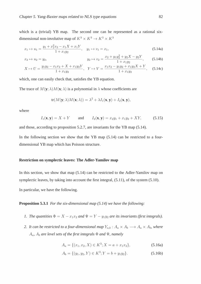
Chapter 5. Yang-Baxter maps related to NLS type equations 82
which is a (trivial) YB map. The second one can be representedas a rational six-
dimensional non-involutive map ofK3 ×K3 → K3 ×K3
x1 7→ u1 =y1 + x21x2 − x1X + x1Y
1 + x1y2, y1 7→ v1 = x1, (5.14a)
x2 7→ u2 = y2, y2 7→ v2 =x2 + y1y
22 + y2X − y2Y
1 + x1y2, (5.14b)
X 7→ U =y1y2 − x1x2 +X + x1y2Y
1 + x1y2, Y 7→ V =
x1x2 − y1y2 + x1y2X + Y
1 + x1y2, (5.14c)
which, one can easily check that, satisfies the YB equation.
The trace ofM(y;λ)M(x;λ) is a polynomial inλ whose coefficients are
tr(M(y;λ)M(x;λ)) = λ2 + λI1(x, y) + I2(x, y),
where
I1(x, y) = X + Y and I2(x, y) = x2y1 + x1y2 +XY, (5.15)
and those, according to proposition 5.2.7, are invariants for the YB map (5.14).
In the following section we show that the YB map (5.14) can be restricted to a four-
dimensional YB map which has Poisson structure.
Restriction on symplectic leaves: The Adler-Yamilov map
In this section, we show that map (5.14) can be restricted to the Adler-Yamilov map on
symplectic leaves, by taking into account the first integral, (5.11), of the system (5.10).
In particular, we have the following.
Proposition 5.3.1 For the six-dimensional map (5.14) we have the following:
1. The quantitiesΦ = X − x1x2 andΨ = Y − y1y2 are its invariants (first integrals).
2. It can be restricted to a four-dimensional mapYa,b : Aa × Ab −→ Aa × Ab, where
Aa, Ab are level sets of the first integralsΦ andΨ, namely
Aa = {(x1, x2, X) ∈ K3;X = a+ x1x2}, (5.16a)
Ab = {(y1, y2, Y ) ∈ K3;Y = b+ y1y2}. (5.16b)

Chapter 5. Yang-Baxter maps related to NLS type equations 83
Moreover, mapYa,b is the Adler-Yamilov map.
Proof
1. It can be readily verified that (5.14) impliesU − u1u2 = X − x1x2 andV − v1v2 =
Y − y1y2. Thus,Φ andΨ are invariants, i.e. first integrals of the map.
2. The existence of the restriction is obvious. Using the conditionsX = x1x2 + a
andY = y1y2 + b, one can eliminateX andY from (5.14). The resulting map,
x→ u(x, y), y→ v(x, y), is given by
(x, y)Ya,b
−→
(
y1 −a− b
1 + x1y2x1, y2, x1, x2 +
a− b
1 + x1y2y2
)
. (5.17)
Map (5.17) coincides with the Adler-Yamilov map.✷
Map (5.17) originally appeared in the work of Adler and Yamilov [10]. Moreover, it
appears as a YB map in [51, 76].
Now, one can use the conditionX = x1x2+a to eliminateX from the Lax matrix (5.12),
i.e.
M(x; a, λ) = λ
1 0
0 0
+
a+ x1x2 x1
x2 1
, x = (x1, x2). (5.18)
The form of Lax matrix (5.18) coincides with the well known Darboux transformation
for the NLS equation (see [80] and references therein). Now,Adler-Yamilov map follows
from the strong Lax representation
M(u; a, λ)M(v; b, λ) =M(y; b, λ)M(x; a, λ). (5.19)
Therefore, the Adler-Yamilov map (5.17) is a reversible parametric YB map with strong
Lax matrix (5.18). Moreover, it is easy to verify that it is not involutive.
For the integrability of this map we have the following
Proposition 5.3.2 The Adler-Yamilov map (5.17) is completely integrable.

Chapter 5. Yang-Baxter maps related to NLS type equations 84
Proof
From the trace ofM(y; b, λ)M(x; a, λ) we obtain the following invariants for the map
(5.17)
I1(x, y) = x1x2 + y1y2 + a+ b, (5.20)
I2(x, y) = (a+ x1x2)(b+ y1y2) + x1y2 + x2y1 + 1. (5.21)
The constant terms inI1, I2 can be omitted. It is easy to check thatI1, I2 are in involution
with respect to a Poisson bracket defined as
{x1, x2} = {y1, y2} = 1, and all the rest {xi, yj} = 0, (5.22)
and the corresponding Poisson matrix is invariant under theYB map (5.17). Therefore
the map (5.17) is completely integrable.✷
The above proposition implies the following.
Corollary 5.3.3 The invariant leavesAa andBb, given in (5.16), are symplectic.
5.3.2 Derivative NLS equation:Z2 reduction
Recall that the Lax operator for the DNLS equation [18, 47] is given by
L(p, q;λ) = Dx+λ2U2+λU1, where U2 = σ3, U1 =
0 2p
2q 0
, (5.23)
andσ3 is a Pauli matrix. The operatorL is invariant with respect to the following
L(λ)→ σ3L(−λ)σ3, (5.24)
whereL(λ) ≡ L(p, q;λ). In particular, the involution (5.24) generates the so-called
reduction group [64, 59] and it is isomorphic toZ2.
The Darboux matrix in this case is given by
M := λ2
f 0
0 0
+ λ
0 fp
fq10 0
+
c 0
0 1
, (5.25)
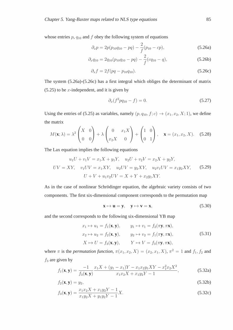
Chapter 5. Yang-Baxter maps related to NLS type equations 85
whose entriesp, q10 andf obey the following system of equations
∂xp = 2p(p10q10 − pq)−2
f(p10 − cp), (5.26a)
∂xq10 = 2q10(p10q10 − pq)−2
f(cq10 − q), (5.26b)
∂xf = 2f(pq − p10q10). (5.26c)
The system (5.26a)-(5.26c) has a first integral which obliges the determinant of matrix
(5.25) to bex-independent, and it is given by
∂x(f2pq10 − f) = 0. (5.27)
Using the entries of (5.25) as variables, namely(p, q10, f ; c) → (x1, x2, X; 1), we define
the matrix
M(x;λ) = λ2
X 0
0 0
+ λ
0 x1X
x2X 0
+
1 0
0 1
, x = (x1, x2, X). (5.28)
The Lax equation implies the following equations
u1U + v1V = x1X + y1Y, u2U + v2V = x2X + y2Y,
UV = XY, v1UV = x1XY, u2UV = y2XY, u2v1UV = x1y2XY,
U + V + u1v2UV = X + Y + x2y1XY.
(5.29)
As in the case of nonlinear Schrodinger equation, the algebraic variety consists of two
components. The first six-dimensional component corresponds to the permutation map
x 7→ u = y, y 7→ v = x, (5.30)
and the second corresponds to the following six-dimensional YB map
x1 7→ u1 = f1(x, y), y1 7→ v1 = f2(πy, πx),
x2 7→ u2 = f2(x, y), y2 7→ v2 = f1(πy, πx),
X 7→ U = f3(x, y), Y 7→ V = f3(πy, πx),
(5.31)
whereπ is thepermutation function, π(x1, x2, X) = (x2, x1, X), π2 = 1 andf1, f2 and
f3 are given by
f1(x, y) =−1
f3(x, y)x1X + (y1 − x1)Y − x1x2y1XY − x
21x2X
2
x1x2X + x1y2Y − 1, (5.32a)
f2(x, y) = y2, (5.32b)
f3(x, y) =x1x2X + x1y2Y − 1
x1y2X + y1y2Y − 1X. (5.32c)

Chapter 5. Yang-Baxter maps related to NLS type equations 86
One can verify that the above map is a non-involutive YB map. The invariants of this map
are given by
I1(x, y) = XY and I2(x, y) = (x · πy)XY +X + Y. (5.33)
The mapY : K3×K3 → K3×K3, given by{(5.31), (5.32a)−(5.32c)}, can be restricted
to a map of the Cartesian product of two two-dimensional affinevarieties
Aa ={
(x1, x2, X) ∈ K3;X −X2x1x2 = a ∈ K}
, (5.34a)
Ab ={
(y1, y2, Y ) ∈ K3;Y − Y 2y1y2 = b ∈ K}
, (5.34b)
which are invariant varieties of the mapY . Thus, the YB map,Ya,b, is a birational map
Ya,b : Aa × Ab → Aa × Ab.
It is easy to uniformise the rational varietyAa and express the YB map explicitly. The
equations defining the varietiesAa andAb are linear inx1, x2 andy1, y2, respectively.
Hence, we can express
x2 =1
x1X−
a
x1X2, y2 =
1
y1Y−
b
y1Y 2. (5.35)
The resulting map is given by
x1 7→ u1 =h1h2y1, X 7→ U = h2Y, y1 7→ v1 = x1, Y 7→ V =
1
h2X (5.36)
where the quantitieshi, i = 1, 2, are given by
h1 =ay1Y + x1X(a− Y )
ay1Y + x1X(b− Y ), h2 =
ay1Y + x1X(b− Y )
by1Y + x1X(b−X). (5.37)
Nevertheless, in the next section, we present a more symmetric way to parametrise the
varietiesAa, Ab and the Lax matrix.
Z2 reduction: A reducible six-dimensional YB map
Now, let us go back to the Darboux matrix (5.25) and replace(fp, fq10, f ; c) →
(x1, x2, X; 1), namely
M(x;λ) = λ2
X 0
0 0
+ λ
0 x1
x2 0
+
1 0
0 1
, x = (x1, x2, X). (5.38)

Chapter 5. Yang-Baxter maps related to NLS type equations 87
From the Lax equation we obtain the following equations
u2v1 = x1y2, u2V = Xy2, Uv1 = x1Y, UV = XY
u1 + v1 = x1 + y1, U + u1v2 + V = X + x2y1 + Y, u2 + v2 = x2 + y2.
Now, the first six-dimensional component of the algebraic variety corresponds to the
trivial map (5.30) and the second component corresponds to amap of the form (5.31),
with f1, f2 andf3 now given by
f1(x, y) =(x1 + y1)X − x1Y − x1x2(x1 + y1)
X − x1(x2 + y2), (5.39a)
f2(x, y) =X − x1(x2 + y2)
Y − y2(x1 + y1)y2, (5.39b)
f3(x, y) =X − x1(x2 + y2)
Y − y2(x1 + y1)Y. (5.39c)
This map has the following invariants
I1(x, y) = XY, I2(x, y) = x · πy +X + Y, (5.40a)
I3(x, y) = x1 + y1, I4(x, y) = x2 + y2. (5.40b)
Restriction on invariant leaves
In this section, we show that the map given by (5.31) and (5.39a)-(5.39c) can be restricted
to a completely integrable four-dimensional map on invariant leaves. As in the previous
section, the idea of this restriction is motivated by the existence of the first integral of the
system (5.26a)-(5.26c),
f − (fp)(fq10) = k = constant, (5.41)
Particularly, we have the following.
Proposition 5.3.4 For the six-dimensional map{(5.31), (5.39a)− (5.39c)} we have the
following:
1. The quantitiesΦ = X − x1x2 andΨ = Y − y1y2 are its first integrals.

Chapter 5. Yang-Baxter maps related to NLS type equations 88
2. It can be restricted to a four-dimensional mapYa,b : Aa × Ab −→ Aa × Ab, given
by
(x, y)Ya,b
−→
(
y1 +a− b
a− x1y2x1,
a− x1y2b− x1y2
y2,b− x1y2a− x1y2
x1, x2 +b− a
b− x1y2y2
)
, (5.42)
andAa, Ab are given by (5.16).
Proof
1. Map{(5.31), (5.39a)− (5.39c)} impliesU − u1u2 = X − x1x2 andV − v1v2 =
Y − y1y2. Therefore,Φ andΨ are first integrals of the map.
2. The conditionsX = x1x2 + a andY = y1y2 + b define the level sets,Aa andAb,
of Φ andΨ, respectively. Using these conditions, we can eliminateX andY from
map{(5.31), (5.39a)− (5.39c)}. The resulting map,Ya,b : Aa × Ab −→ Aa × Ab,
is given by (5.42).
✷
Now, using conditionX = x1x2 + a, matrix (5.38) takes the following form
M(x; k;λ) = λ2
k + x1x2 0
0 0
+ λ
0 x1
x2 0
+
1 0
0 1
. (5.43)
Now, map (5.42) follows from the strong Lax representation (5.19). Therefore, it is
reversible parametric YB map. It can also be verified that it is not involutive.
For the integrability of map (5.42) we have the following
Proposition 5.3.5 Map (5.42) is completely integrable.
Proof
The invariants of map (5.42) which we retrieve from the traceofM(y; b, λ)M(x; a, λ) are
I1(x, y) = (a+ x1x2)(b+ y1y2), I2(x, y) = (x1 + y1)(x2 + y2) + a+ b. (5.44)

Chapter 5. Yang-Baxter maps related to NLS type equations 89
However, the quantitiesx1 + y1 andx2 + y2 in I2 are invariants themselves. The Poisson
bracket in this case is given by
{x1, x2} = {y1, y2} = {x2, y1} = {y2, x1} = 1, and all the rest {xi, yj} = 0.
(5.45)
The rank of the Poisson matrix is 2,I1 is one invariant andI2 = C1C2 + a + b, where
C1 = x1 + y1 andC2 = x2 + y2 are Casimir functions. The latter are preserved by (5.42),
namelyCi ◦ Ya,b = Ci, i = 1, 2. Therefore, map (5.42) is completely integrable.✷
Corollary 5.3.6 Map (5.42) can be expressed as a map of two variables on the symplectic
leaf
x1 + y1 = c1, x2 + y2 = c2. (5.46)
5.3.3 A deformation of the DNLS equation: Dihedral Group
Recall that, in the case of the deformation of the DNLS equation, the Lax operator is
given by
L(p, q;λ) = Dx + λ2U2 + λU1 + λ−1U−1 − λ−2U−2, where
U2 ≡ U−2 = σ3, U1 =
0 2p
2q 0
, U−1 = σ1U1σ1,(5.47)
andσ1, σ3 are Pauli matrices. Here, the reduction group consists of the following set of
transformations acting on the Lax operator (5.47) ,
L(λ)→ σ3L(−λ)σ3 and L(λ)→ σ1L(λ−1)σ1, (5.48)
and it is isomorphic toZ2 × Z2∼= D2, [59].
In this case, the Darboux matrix is given by
M = f
λ2 0
0 λ−2
+ λ
0 p
q10 0
+ g
1 0
0 1
+1
λ
0 q10
p 0
, (5.49)
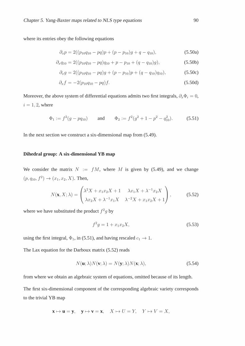
Chapter 5. Yang-Baxter maps related to NLS type equations 90
where its entries obey the following equations
∂xp = 2((p10q10 − pq)p+ (p− p10)g + q − q10), (5.50a)
∂xq10 = 2((p10q10 − pq)q10 + p− p10 + (q − q10)g), (5.50b)
∂xg = 2((p10q10 − pq)g + (p− p10)p+ (q − q10)q10), (5.50c)
∂xf = −2(p10q10 − pq)f. (5.50d)
Moreover, the above system of differential equations admits two first integrals,∂xΦi = 0,
i = 1, 2, where
Φ1 := f 2(g − pq10) and Φ2 := f 2(g2 + 1− p2 − q210). (5.51)
In the next section we construct a six-dimensional map from (5.49).
Dihedral group: A six-dimensional YB map
We consider the matrixN := fM , whereM is given by (5.49), and we change
(p, q10, f2)→ (x1, x2, X). Then,
N(x, X;λ) =
λ2X + x1x2X + 1 λx1X + λ−1x2X
λx2X + λ−1x1X λ−2X + x1x2X + 1
, (5.52)
where we have substituted the productf 2g by
f 2g = 1 + x1x2X, (5.53)
using the first integral,Φ1, in (5.51), and having rescaledc1 → 1.
The Lax equation for the Darboux matrix (5.52) reads
N(u;λ)N(v;λ) = N(y;λ)N(x;λ), (5.54)
from where we obtain an algebraic system of equations, omitted because of its length.
The first six-dimensional component of the corresponding algebraic variety corresponds
to the trivial YB map
x 7→ u = y, y 7→ v = x, X 7→ U = Y, Y 7→ V = X,

Chapter 5. Yang-Baxter maps related to NLS type equations 91
and the second component corresponds to the following map
x1 7→ u1 =f(x, y)g(x, y)
, y1 7→ v1 = x1,
x2 7→ u2 = y2, y2 7→ v2 =f(πy, πx)g(πy, πx)
, (5.55)
X 7→ U =g(x, y)h(x, y)
, Y 7→ V =g(πy, πx)h(πy, πx)
,
wheref, g andh are given by
f(x, y) = x1X + [x2 − y2 + 2x1x2y1 + x21(y2 − 3x2)]XY+
(y22 − 1)[y1(1 + x21)− x1(1 + y21)]XY2 − (x21 − 1)(y2 − x2)X
2−
(x21 − 1)[x22(3x1 − y1)− x1 − y1 + 2y2(y1y2 − x1x2)]X2Y− (5.56a)
(x21 − 1)(y22 − 1)[y2(y21 − 1) + x2(y
21 − 2x1y1 + 1)]X2Y 2+
y1(x21 − 1)2(x22 − 1)(y22 − 1)X3Y 2 + (x21 − 1)2(x22 − 1)(y2 − x2)X
3Y+
(y1 − x1)Y,
g(x, y) = X + 2y2(y1 − x1)XY + (y22 − 1)(x1 − y1)2XY 2+
2(x21 − 1)(1− x2y2)X2Y + 2x2(x
21 − 1)(y22 − 1)(x1 − y1)X
2Y 2+ (5.56b)
(x21 − 1)2(x22 − 1)(y22 − 1)X3Y 2
and
h(x, y) = 1− 2x1(y2 − x2)X − 2(x1y1 − 1)(y22 − 1)XY+
(x21 − 1)(x2 − y2)2X2 − 2y1(x2 − y2)(x
21 − 1)(y22 − 1)X2Y+ (5.56c)
(x21 − 1)(y21 − 1)(y22 − 1)2X2Y 2.
It can be verified that this is a YB map. From tr(N(x, X;λ)N(y, Y ;λ)) we extract the
following invariants for the above map
I1(x, y) = XY, (5.57a)
I2(x, y) = X + Y + (x1 + y1)(x2 + y2)XY, (5.57b)
I3(x, y) = 2x1x2X + 2y1y2Y + 2(x · y + x1x2y1y2)XY + 2. (5.57c)

Chapter 5. Yang-Baxter maps related to NLS type equations 92
5.3.4 Dihedral group: A linearised YB map
In the cases of the NLS and DNLS equations we were able to derive six-dimensional
maps and, using their invariants, reduce them to four-dimensional YB maps. The matrix
refactorisation (4.12) for matrix (5.49) is not unique and it is difficult to deduce a six-
dimensional YB map in this case. Therefore, even though we can reuniformise equations
(5.51), we can not use them to derive a four-dimensional map.Yet, we can find a linear
approximation to the former.
In particular, let us replace(fq10, fp) → (ǫx1, ǫx2) in the Darboux matrix (5.49) and
linearise the corresponding map aroundǫ = 0.
It follows fromΦ1 =1−k2
4andΦ2 =
1+k2
2that the quantitiesf andfg are given by
f =1 + k
2+O(ǫ) and fg =
1− k
2+O(ǫ),
and, therefore, the Lax matrix by
M =1 + k
2
λ2 0
0 λ−2
+
0 λx1 + λ−1x2
λx2 + λ−1x1 0
+1− k
2
1 0
0 1
+O(ǫ).
The linear approximation to the YB map is given by
x1
x2
y1
y2
U0−→
u1
u2
v1
v2
=
(a−1)(a−b)(a+1)(a+b)
a−ba+b
2aa+b
(a+1)(b−a)(b+1)(a+b)
0 0 0 a+1b+1
b+1a+1
0 0 0
(a−b)(b+1)(a+1)(a+b)
2ba+b
b−aa+b
(b−1)(b−a)(b+1)(a+b)
x1
x2
y1
y2
(5.58)
which is a linear parametric YB map and it is not involutive.
5.4 2N × 2N -dimensional YB maps
In this section, we consider the vector generalisations of the YB maps (5.17) and (5.42).
We replace the variables,x1 andx2, in the Lax matrices withN -vectorsw1 andwT2 to
obtain2N × 2N YB maps.

Chapter 5. Yang-Baxter maps related to NLS type equations 93
In what follows we use the following notation for an-vectorw = (w1, ..., wn)
w = (w1,w2), where w1 = (w1, ..., wN ), w2 = (wN+1, ..., w2N ) (5.59)
and also
〈ui| := ui, |wi〉 := wTi and their dot product with 〈ui, wi〉. (5.60)
5.4.1 NLS equation
Replacing the variables in (5.18) withN -vectors, namely
M(w; a, λ) =
λ+ a+ 〈w1, w2〉 〈w1|
|w2〉 I
, (5.61)
we obtain a unique solution of the Lax equation given by the following 2N × 2N map
〈u1| = 〈y1|+ f(z; a, b)〈x1|,
〈u2| = 〈y2|,
(5.62a)
and
〈v1| = 〈x1|,
〈v2| = 〈x2|+ f(z; b, a)〈y2|,
(5.62b)
wheref is given by
f(z; b, a) =b− a
1 + z, z := 〈x1, y2〉. (5.62c)
The above is a non-involutive parametric2N ×2N YB map with strong Lax matrix given
by (5.61). As a YB map it appears in [76], but it is originally introduced by Adler [6].
Moreover, one can construct the above2N × 2N map for theN × N Darboux matrix
(5.61) by taking the limit of the solution of the refactorisation problem in [53].
Two invariants of this map are given by
I1(x, y; a, b) = 〈x1, x2〉+ 〈y1, y2〉, (5.63a)
I2(x, y; a, b) = b〈x1, x2〉+ a〈y1, y2〉+ 〈x1, y2〉+ 〈x2, y1〉+ 〈x1, x2〉〈y1, y2〉. (5.63b)
These are the invariants which are obtained from the trace ofM(y; b, λ)M(x; a, λ) and
they are not enough to claim Liouville integrability.

Chapter 5. Yang-Baxter maps related to NLS type equations 94
5.4.2 Z2 reduction
In the case ofZ2 we consider, instead of (5.43), the following matrix
M(w; a, λ) =
λ2(a+ 〈w1, w2〉) λ〈w1|
λ|w2〉 I
, (5.64)
we obtain a unique solution for the Lax equation given by the following 2N × 2N map
〈u1| = 〈y1|+ f(z; a, b)〈x1|,
〈u2| = g(z; a, b)〈y2|,
(5.65a)
and
〈v1| = g(z; b, a)〈x1|,
〈v2| = 〈x2|+ f(z; b, a)〈y2|,
(5.65b)
wheref andg are given by
f(z; a, b) =a− b
a− z, g(z; a, b) =
a− z
b− z, z := 〈x1, y2〉. (5.65c)
The above map is a non-involutive parametric2N × 2N YB map with strong Lax matrix
given by (5.64).
It follows from the trace ofM(y; b, λ)M(x; a, λ), that two invariants for (5.65a)-(5.65b)
are given by
I1(x, y; a, b) = b〈x1, x2〉+ a〈y1, y2〉+ 〈x1, x2〉〈y1, y2〉, (5.66a)
I2(x, y; a, b) = 〈x1 + y1, x2 + y2〉. (5.66b)
In fact, both vectors of the inner product inI2 are invariants.
However, as in the case of the NLS vector generalisation, theinvariants are not enough to
claim Liouville integrability.

95
Chapter 6
Extensions on Grassmann algebras
6.1 Overview
Noncommutative extensions of integrable equations have been of great interest since late
seventies; for instance, in [19] the supersymmetric Liouville and sine-Gordon equations
were studied, while in [54] hierarchies of the KdV equation were associated to super Lie
algebras. Other examples include the NLS, the DNLS and KP equations etc. Indicatively,
we refer to [11, 29, 30, 73].
In this chapter, motivated by [38], we are interested in the Grassmann extensions of some
of the Darboux matrices and their associated YB maps presented in the previous chapters.
Specifically, we shall present noncommutative extensions of the Darboux matrices in the
cases of the NLS equation and the DNLS equation, together with the noncommutative
extensions of the associated YB maps. In fact, we will use theDarboux matrices to
construct ten-dimensional YB maps which can be restricted to eight-dimensional YB
maps on invariant leaves.
The chapter is organised as follows: In the next section we present the basic facts and
properties of Grassmann algebras which we will need in the following sections. Section 3
deals with the noncommutative extensions of the Darboux matrices of NLS type equations
and, particularly, the Grassmann extension of the Darboux matrix in the cases of the
NLS equation [38] and the DNLS equation. Section 4 is devotedto the construction
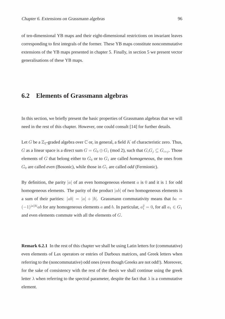
Chapter 6. Extensions on Grassmann algebras 96
of ten-dimensional YB maps and their eight-dimensional restrictions on invariant leaves
corresponding to first integrals of the former. These YB mapsconstitute noncommutative
extensions of the YB maps presented in chapter 5. Finally, insection 5 we present vector
generalisations of these YB maps.
6.2 Elements of Grassmann algebras
In this section, we briefly present the basic properties of Grassmann algebras that we will
need in the rest of this chapter. However, one could consult [14] for further details.
LetG be aZ2-graded algebra overC or, in general, a fieldK of characteristic zero. Thus,
G as a linear space is a direct sumG = G0 ⊕G1 (mod 2), such thatGiGj ⊆ Gi+j. Those
elements ofG that belong either toG0 or toG1 are calledhomogeneous, the ones from
G0 are calledeven(Bosonic), while those inG1 are calledodd (Fermionic).
By definition, the parity|a| of an even homogeneous elementa is 0 and it is1 for odd
homogeneous elements. The parity of the product|ab| of two homogeneous elements is
a sum of their parities:|ab| = |a| + |b|. Grassmann commutativity means thatba =
(−1)|a||b|ab for any homogeneous elementsa andb. In particular,a21 = 0, for all a1 ∈ G1
and even elements commute with all the elements ofG.
Remark 6.2.1 In the rest of this chapter we shall be using Latin letters for(commutative)
even elements of Lax operators or entries of Darboux matrices, and Greek letters when
referring to the (noncommutative) odd ones (even though Greeks are not odd!). Moreover,
for the sake of consistency with the rest of the thesis we shall continue using the greek
letterλ when referring to the spectral parameter, despite the fact thatλ is a commutative
element.

Chapter 6. Extensions on Grassmann algebras 97
6.2.1 Supertrace and superdeterminant
LetM be a square matrix of the following form
M =
P Π
Λ L
, (6.1)
whereP andL are square matrices of even variables, whereasΠ andΛ are matrices of
odd variables, not necessarily square.
We define thesupertraceof M –and we will denote it by str(M)– to be the following
quantity
str(M) = tr(P )− tr(L), (6.2)
where tr(.) is the usual trace of a matrix.
Moreover, we define thesuperdeterminantof M –and we will denote it by sdet(M)– to
be
sdet(M) = det(P − ΠL−1Λ) det(L−1) = (6.3a)
= det(P−1) det(L− ΛP−1Π), (6.3b)
wheredet(.) is the usual determinant of a matrix.
The simplest properties of the supertrace and the superdeterminant, for two matricesA
andB of the form (6.1), are the following
1. str(AB)=str(BA),
2. sdet(AB)=sdet(A)sdet(B).
6.2.2 Differentiation rule for odd variables
The (left) derivative of a product of odd elements, sayαi1 , . . . , αik , obeys the following
rule
∂
∂αi
(αi1 · . . . · αik) = δii1αi2αi3 · . . . · αik −
δii2αi1αi3 · . . . · αik + δii3αi1αi2 · . . . · αik − . . . (6.4)

Chapter 6. Extensions on Grassmann algebras 98
whereδij is the Kronecker operator. For example, ifα andβ are odd variables, then
∂
∂α(αβ) = β, but
∂
∂β(αβ) = −α. (6.5)
6.2.3 Properties of the Lax equation
Let L = L(x, χ; a) be a Lax matrix wherex is an even variable,χ is an odd variable and
a a parameter. Since the Lax equation,
L(u, ξ; a)L(v, η; b) = L(y, ψ; b)L(x, χ; a) (6.6)
has the obvious symmetry
(u, ξ, v, η, a, b)←→ (y, ψ, x, χ, b, a) (6.7)
we have the following
Proposition 6.2.2 If a matrix refactorisation problem (6.6) yields a rationalmap
(x, χ, y, ψ) = Ya,b(u, ξ, v, η), then this map is birational.
Proof
Let Y : (x, χ, y, ψ) 7→ (u, ξ, v, η) be a rational map corresponding to a refactorisation
problem (4.12), i.e.
x 7→ u =n1(x, χ, y, ψ; a, b)
d1(x, χ, y, ψ; a, b), y 7→ v =
n2(x, χ, y, ψ; a, b)
d2(x, χ, y, ψ; a, b), (6.8a)
χ 7→ ξ =n3(x, χ, y, ψ; a, b)
d3(x, χ, y, ψ; a, b), ψ 7→ η =
n4(x, χ, y, ψ; a, b)
d4(x, χ, y, ψ; a, b), (6.8b)
whereni, di, i = 1, 2, 3, 4, are polynomial functions of their variables.
Due to the symmetry (6.7) of the refactorisation problem (6.6), the inverse map ofY ,
Y −1 : (x, χ, y, ψ) 7→ (u, ξ, v, η), is also rational and, in fact,
u 7→ x =n1(v, η, u, ξ; b, a)
d1(v, η, u, ξ; b, a), v 7→ y =
n2(v, η, u, ξ; b, a)
d2(v, η, u, ξ; b, a), (6.9a)
ξ 7→ χ =n3(v, η, u, ξ; b, a)
d3(v, η, u, ξ; b, a), η 7→ ψ =
n4(v, η, u, ξ; b, a)
d4(v, η, u, ξ; b, a). (6.9b)
Therefore,Y is a birational map.✷

Chapter 6. Extensions on Grassmann algebras 99
Remark 6.2.3 Functionsdi(x, χ, y, ψ; a, b), i = 1, 2, 3, 4, must depend on the odd
variables in a way such that their expressions are even. For example, the expression
xy + χψ is even.
Proposition 6.2.4 If L = L(x, χ, a;λ) is a Lax matrix with corresponding YB map,Y :
(x, χ, y, ψ) 7→ (u, ξ, v, η), then str(L(y, ψ, b;λ)L(x, χ, a;λ)) is a generating function of
invariants of the YB map.
Proof
Since,
str(L(u, ξ, a;λ)L(v, η, b;λ))(4.12)= str(L(y, ψ, b;λ)L(x, χ, a;λ))
= str(L(x, χ, a;λ)L(y, ψ, b;λ)), (6.10)
and function str(L(x, χ, a;λ)L(y, ψ, b;λ)) can be written as str(L(x, χ, a;λ)L(y, ψ, b;λ))
=∑
k
λkIk(x, χ, y, ψ; a, b), from (6.10) follows that
Ii(u, ξ, v, η; a, b) = Ii(x, χ, y, ψ; a, b), (6.11)
which are invariants forY . ✷
Remark 6.2.5 The invariants of a YB map,Ii(x, χ, y, ψ; a, b), may not be functionally
independent.
6.3 Extensions of Darboux transformations on Grass-
mann algebras
In this section we consider the Grassmann extensions of the Darboux matrices
corresponding to the NLS equation and the DNLS equation. In particular, we present the
noncommutative extension of Darboux matrices (3.36) (see [38]) and (3.54) (see [37]).

Chapter 6. Extensions on Grassmann algebras 100
6.3.1 Nonlinear Schrodinger equation
The Grassmann extension of the Darboux matrix (3.36) was constructed in [38]. We
present this Darboux matrix together with its associated Lax operator and we will use it
in the next section to construct a Grassmann extension of theAdler-Yamilov map.
Specifically, let us consider a more general Lax operator than (3.33), namely the following
noncommutative extension of the NLS operator
L := Dx + U(p, q, ψ, φ, ζ, κ;λ) = Dx + λU1 + U0, (6.12a)
whereU1 andU0 are given by
U1 = diag(1,−1, 0), U0 =
0 2p θ
2q 0 ζ
φ κ 0
, (6.12b)
wherep, q ∈ G0 andψ, φ, ζ, κ ∈ G1. Note that, if we set the odd variables equal to zero,
operator (6.12) coincides with (3.33).
A linear in the spectral parameter Darboux matrix for (3.33)is given by the following
[38].
Proposition 6.3.1 LetM = λM1+M0 be a Darboux matrix for (6.12). Moreover, letM
define a Darboux transformation of rank 1. Then, up to a gauge transformation,M is of
the following form
M(p, q, θ, φ; c1, c2) =
F + λ p θ
q10 c1 0
φ10 0 c2
, (6.13)
wherec1 and c2 can be either 1 or 0. In the case wherec1 = c2 = 1, the entries of

Chapter 6. Extensions on Grassmann algebras 101
M(p, q, θ, φ; 1, 1) satisfy the following system of differential-difference equations
Fx = 2(pq − p10q10) + θφ− θ10φ10, (6.14a)
px = 2(Fp− p10) + θζ, (6.14b)
q10,x = 2(q − q10F )− κ10φ10, (6.14c)
θx = Fθ − θ10 + pκ, (6.14d)
φ10,x = φ− φ10F − ζ10q10, (6.14e)
and the algebraic equations
θq10 = (S − 1)κ, (6.15a)
φ10p = (S − 1)ζ. (6.15b)
Proof
Substitution ofM to equation (3.9) implies a second order algebraic equationin λ.
Equating the coefficients of the several powers ofλ equal to zero, we obtain the following
system of equations
λ2 :[
U1,M1
]
= 0, (6.16a)
λ1 : M1,x +[
U1,M0
]
+ U010M1 −M1U
0 = 0, (6.16b)
λ0 : M0,x + U010M0 −M0U
0 = 0. (6.16c)
The first equation, (6.16a), implies thatM1 must be diagonal, sayM1 = diag(α, β, γ).
Then, from the diagonal part of (6.16b) we deduce thatαx = βx = γx = 0. Since
rank(M1) = 1, only one ofα, β andγ can be nonzero. Without any loss of generality,
we chooseα = 1 andβ = γ = 0.
Now, the off-diagonal part of (6.16b) impliesM0,12 = p,M0,13 = θ,M0,21 = q10,M0,31 =
φ10 andM0,32 =M0,23 = 0. We call theM0,11 entryM0,11 = F .
Finally, from equation (6.16c) we obtain(M0,22)x = (M0,33)x = 0, namelyM0,22 = c1,
M0,22 = c2, together with equations (6.14).✷

Chapter 6. Extensions on Grassmann algebras 102
Note 6.3.2 At this point, it is worth mentioning that the superdeterminant of matrix
M(p, q, θ, φ; 1, 1) in (6.13) implies the following
∂x(F − pq10 − φ10θ) = 0, (6.17)
since∂x(sdet(M)) = 0. Moreover, (6.17) is a first integral for system (6.14) forc1 =
c2 = 1.
Remark 6.3.3 If one sets the odd variables equal to zero, matrix (6.13) theresults of
Proposition 6.3.1 agree with those in Proposition 3.4.1 presented in chapter 3.
6.3.2 Derivative nonlinear Schrodinger equation
Let us now consider a more general than (3.49), namely the following noncommutative
extension of the DNLS operator
L = Dx + λ2U2 + λU1, (6.18a)
where
U2 =diag(1,−1,−1) and U1 =
0 2p 2θ
2q 0 0
2φ 0 0
. (6.18b)
Operator (6.18) is invariant under the transformation
s1(λ) : L(λ)→ L(−λ) = s3L(λ)s3, (6.19)
wheres3 = diag(1,−1,−1), s23 = 1.
We are seeking a Darboux matrix for (6.18) with square dependence in the spectral
parameter, namely of the form
M = λ2M2 + λM1 +M0, (6.20)
whereMi, i = 0, 1, 2, is a3× 3 matrix.

Chapter 6. Extensions on Grassmann algebras 103
Lemma 6.3.4 LetM be a second order matrix polynomial inλ of the form (6.20). Then,
M is invariant under the involutions1(λ) iff
Mi,12 =Mi,13 =Mi,21 =Mi,31 = 0, i = 0, 2, and (6.21a)
M1,11 =M1,22 =M1,33 =M1,23 =M1,32 = 0. (6.21b)
Proof
It can be readily proven fromM(−λ) = s3M(λ)s3. ✷
We restrict ourselves to the case whereM2 in (6.20) has rank one.
Proposition 6.3.5 Let M be a Darboux matrix for (6.18) of the form (6.20), with
rankM2 = 1, and suppose that it is invariant under the involution (6.19). Then, up
to a gauge transformation,M is given by
M(f, p, q10, θ, φ10; c1, c2) = λ2
f 0 0
0 0 0
0 0 0
+ λ
0 fp fθ
q10f 0 0
φ10f 0 0
+
c1 0 0
0 1 0
0 0 c2
, (6.22)
where its entries satisfy the following differential-difference equations
fx = 2f(pq − p10q10θφ− θ10φ10), (6.23a)
px = 2p(p10q10 − pq + θ10φ10 − θφ)− 2c2p10 − c1p
f, (6.23b)
q10,x = 2q10(p10q10 − pq + θ10φ10 − θφ)− 2c1q10 − c2q
f, (6.23c)
θx = 2φ(p10q10 − pq + θ10φ10 − θφ) +c1θ − c2θ10
f, (6.23d)
φ10,x = 2φ10(p10q10 − pq + θ10φ10 − θφ) +c2φ− c1φ10
f. (6.23e)
Proof
First of all, for the entries of matricesMi, i = 1, 2, 3 we have (6.21). Then, substitution
of M to equation (3.9) implies a second order algebraic equationin λ. Equating the
coefficients of the several powers ofλ equal to zero, we obtain the following system of

Chapter 6. Extensions on Grassmann algebras 104
equations
[
U2,M2
]
= 0 (6.24a)[
U2,M1
]
+ U110M2 −M2U
1 = 0 (6.24b)
M2,x +[
U2,M0
]
+ U110M1 −M1U
1 = 0 (6.24c)
M1,x + U110M0 −M0U
1 = 0 (6.24d)
M0,x = 0. (6.24e)
From (6.24e) follows that the matrixM0 must be constant, whereas equation (6.24a)
implies thatM2 is diagonal. SincerankM2 = 1 we can chooseM2 = diag{f, 0, 0}
without loss of generality; the casesM2 = diag{0, g, 0} andM2 = diag{0, 0, h} lead to
gauge equivalent Darboux matrices. In this case, from equation (6.24b) we have that the
entries ofM1 are given by
M1,12 = fp, M1,13 = fθ, M1,21 = q10f and M1,31 = φ10f. (6.25)
Now, from equation (6.24c) we deduce equation (6.23a) and thatM0 must be diagonal,
namely of the formM0 = diag(c1, 1, c2) (one of the parameters along its diagonal can be
rescaled to 1). Therefore, matrixM is of the form (6.22).
Finally, equation (6.24d) implies system (6.23b)-(6.23e)(where we have made use of
(6.23a)).✷
Note 6.3.6 Entry f is permitted to appear in the denominator in (6.23), as it is an
even variable. This is due to the superdeterminant of matrixM . In fact, the constant
determinant property of matrixM(f, p, q10, θ, φ10; 1, 1) implies the following equation
∂x(f − f2(pq10 + θφ10)) = 0, (6.26)
which makes it quite obvious thatf must be even. Moreover, (6.26) is a first integral for
the system of differential-difference equations (6.23).
Remark 6.3.7 The results of Proposition 6.3.5 agree with those of Proposition 3.4.3 if
one sets the odd variables equal to zero.

Chapter 6. Extensions on Grassmann algebras 105
6.4 Grassmann extensions of Yang-Baxter maps
Here we employ the Darboux matrices presented in the previous section to construct ten-
dimensional YB maps, which can be restricted to eight-dimensional YB maps on invariant
leaves. We start with the case of NLS equation.
6.4.1 Nonlinear Schrodinger equation
According to (6.13) we define the following matrix
M(x;λ) =
X + λ x1 χ1
x2 1 0
χ2 0 1
, x := (x1, x2, χ1, χ2, X), (6.27)
and substitute to the Lax equation.
The corresponding algebraic variety is a union of two ten-dimensional components. The
first one is obvious from the refactorisation problem, and itcorresponds to the permutation
map
x 7→ u = y, y 7→ v = x,
which is a trivial YB map. The second one can be represented asa ten-dimensional non-
involutive Yang-Baxter map given by
x1 7→ u1 = y1 −X − x1x2 − χ1χ2 − Y + y1y2 + ψ1ψ2
1 + x1y2 + χ1ψ2
x1, (6.28a)
x2 7→ u2 = y2, (6.28b)
χ1 7→ ξ1 = ψ1 −X − x1x2 − Y + y1y2 + ψ1ψ2
1 + x1y2χ1, (6.28c)
χ2 7→ ξ2 = ψ2, (6.28d)
X 7→ U =X − x1x2 − χ1χ2 + (x1y2 + χ1ψ2)Y + y1y2 + ψ1ψ2
1 + x1y2 + χ1ψ2
, (6.28e)
y1 7→ v1 = x1, (6.28f)
y2 7→ v2 = x2 +X − x1x2 − χ1χ2 − Y + y1y2 + ψ1ψ2
1 + x1y2 + χ1ψ2
y2, (6.28g)
ψ1 7→ η1 = χ1, (6.28h)
Chapter 6. Extensions on Grassmann algebras 106
ψ2 7→ η2 = χ2 +X − x1x2 − χ1χ2 − Y + y1y2
1 + x1y2ψ2, (6.28i)
Y 7→ V =(x1y2 + χ1ψ2)X + x1x2 + χ1χ2 + Y − y1y2 − ψ1ψ2
1 + x1y2 + χ1ψ2
. (6.28j)
Finally, map (6.28) is birational due to Proposition 6.2.2.
Restriction on invariant leaves: Extension of Adler-Yamilov map
In this section, we derive an eight-dimensional Yang-Baxtermap from map (6.28). This
is a Grassmann extension of the Adler-Yamilov map [10, 51, 76]. Our proof is motivated
by the existence of the first integral (6.17).
In particular, we have the following
Proposition 6.4.1 1. The quantitiesΦ = X−x1x2−χ1χ2 andΨ = Y −y1y2−ψ1ψ2
are invariants (first integrals) of the map (6.28),
2. The ten-dimensional map (6.28) can be restricted to an eight-dimensional mapYa,b :
Aa × Ab −→ Aa × Ab, whereAa, Ab are level sets of the first integralsΦ andΨ,
namely
Aa = {(x1, x2, χ1, χ2, X) ∈ K5;X = a+ x1x2 + χ1χ2}, (6.29a)
Ab = {(y1, y2, ψ1, ψ2, Y ) ∈ K5;Y = b+ y1y2 + ψ1ψ2}, (6.29b)
3. The bosonic limit of mapYa,b is the Adler-Yamilov map.
Proof
1. It can be readily verified that (6.28) impliesU − u1u2 − ξ1ξ2 = X − x1x2 − χ1χ2
andV − v1v2 − η1η2 = Y − y1y2 − ψ1ψ2. Thus,Φ andΨ are invariants, i.e. first
integrals of the map.

Chapter 6. Extensions on Grassmann algebras 107
2. The existence of the restriction is obvious. Using the conditionsX = x1x2+χ1χ2+
a andY = y1y2 +ψ1ψ2 + b, one can eliminateX andY from (6.28). The resulting
map isx→ u = u(x, y), y→ v = v(x, y), whereu andv are given by
u =
(
y1 +(b− a)(1 + x1y2 − χ1ψ2)
(1 + x1y2)2x1, y2, ψ1 +
b− a
1 + x1y2χ2, ψ2
)
, (6.30a)
v =
(
x1, x2 +(a− b)(1 + x1y2 − χ1ψ2)
(1 + x1y2)2y2, χ1, χ2 +
a− b
1 + x1y2ψ2
)
. (6.30b)
3. If one sets the odd variables of the above map equal to zero,namelyχ1 = χ2 = 0
andψ1 = ψ2 = 0, then the map (6.30) coincides with the Adler-Yamilov map.
✷
Now, one can use the conditionX = x1x2+χ1χ2+a to eliminateX from the Lax matrix
(6.27), i.e.
M(x; a, λ) =
a+ x1x2 + χ1χ2 + λ x1 χ1
x2 1 0
χ2 0 1
, (6.31)
which corresponds to the Darboux matrix derived in [38]. Now, Adler-Yamilov map’s
extension follows from the strong Lax representation
M(u; a, λ)M(v; b, λ) =M(y; b, λ)M(x; a, λ). (6.32)
Therefore, the extension of the Adler-Yamilov’s map (6.30)is a reversible parametric YB
map. Moreover, it is easy to verify that it is not involutive.Birationality of map (6.30) is
due to Prop. 6.2.2.
Now, from str(M(y; b, λ)M(x; a, λ)) we obtain the following invariants for map (6.30)
T1 = a+ b+ x1x2 + y1y2 + χ1χ2 + ψ1ψ2,
T2 = (a+ x1x2 + χ1χ2)(b+ y1y2 + ψ1ψ2) + x1y2 + x2y1 + χ1ψ2 − χ2ψ1,
However, these are linear combinations of the following integrals
I1 =(a+ x1x2 + χ1χ2)(b+ y1y2) + ψ1ψ2(a+ x1x2) + x1y2+
x2y1 + χ1ψ2 − χ2ψ1, (6.33a)
I2 =x1x2 + y1y2, I3 = χ1χ2 + ψ1ψ2, I4 = χ1χ2ψ1ψ2. (6.33b)

Chapter 6. Extensions on Grassmann algebras 108
These are in involution with respect to the Poisson bracket
{x1, x2} = {y1, y2} = 1, {χ1, χ2} = {ψ1, ψ2} = 1 and all the rest
{xi, xj} = {yi, yj} = {xi, yj} = 0.
and the corresponding Poisson matrix is invariant under theYB map (6.30). However, we
cannot make any conclusions about the Liouville integrability of (6.30), asI3 andI4 are
not functionally independent (notice thatI23 = 2I4).
6.4.2 Derivative nonlinear Schrodinger equation
According to matrixM(p, q10, θ, φ10; 1, 1) in (6.22) we consider the following matrix
M(x;λ) = λ2
X 0 0
0 0 0
0 0 0
+ λ
0 x1 χ1
x2 0 0
χ2 0 0
+
1 0 0
0 1 0
0 0 1
, (6.34)
wherex = (x1, x2, χ1, χ2, X) and, in particular, we have set
X := f, x1 := fp, x2 = fq10, χ1 := fθ and χ2 := ψ10f. (6.35)
The Lax equation for the above matrix implies the following equations
U + V + u1v2 + ξ1η2 = Y +X + y1x2 + ψ1χ2, (6.36a)
Uvi = xiY, i = 1, 3, V ui = yiX, i = 2, 4, (6.36b)
ui + vi = xi + yi, i = 1, . . . , 4. (6.36c)
As in the previous section, the algebraic variety consists of two components. The first
ten-dimensional component corresponds to the permutationmap
x 7→ u = y, y 7→ v = x, (6.37)
and the second corresponds to the following ten-dimensional YB map
x 7→ u =
(
y1 +f
gx1,
g
hy2, ψ1 +
f
gχ1,
g
hψ2,
g
hY
)
, (6.38a)
y 7→ v =
(
h
gx1, x2 +
f
hy2,
h
gχ1, χ2 +
f
hψ2,
h
fX
)
. (6.38b)

Chapter 6. Extensions on Grassmann algebras 109
wheref = f(x, y), g = g(x, y) andh = h(x, y) are given by the following expressions
f(x, y) = X − x1x2 − χ1χ2 − Y + y1y2 + ψ1ψ2, (6.39a)
g(x, y) = X − x1(x2 + y2)− χ1(χ2 + ψ2), (6.39b)
h(x, y) = Y − (x1 + y1)y2 − (χ1 + ψ1)ψ2. (6.39c)
6.4.3 Restriction on invariant leaves
In this section, we show that the map given by (6.38)-(6.39) can be restricted to a
completely integrable eight-dimensional YB map on invariant leaves. As in the previous
section, the idea of this restriction is motivated by the first integral (6.26).
Particularly, we have the following
Proposition 6.4.2 1. Φ = X−x1x2−χ1χ2 andΨ = Y −y1y2−ψ1ψ2 are invariants
of the map (6.38)-(6.39),
2. The ten-dimensional map (6.38)-(6.39) can be restrictedto an eight-dimensional
mapYa,b : Aa × Ab −→ Aa × Ab, whereAa, Ab are given by (6.29).
3. The bosonic limit of the above eight-dimensional map is map (5.42), corresponding
to the DNLS equation.
Proof
1. Map (6.38)-(6.39) impliesU−u1u2−ξ1ξ2 = X−x1x2−χ1χ2 andV −v1v2−η1η2 =
Y − y1y2 − ψ1ψ2. Therefore,Φ andΨ are first integrals of the map.
2. The conditionsX = x1x2 + χ1χ2 + a andY = y1y2 + ψ1ψ2 + b define the level
sets,Aa andAb, of Φ andΨ, respectively. Using these conditions, we can eliminate
X andY from map (6.38)-(6.39). The resulting map,Ya,b : Aa ×Ab −→ Aa ×Ab,

Chapter 6. Extensions on Grassmann algebras 110
is given by
x1 7→ u1 = y1 +(a− b)(a− x1y2 + χ1ψ2)
(a− x1y2)2x1, (6.40a)
x2 7→ u2 =(a− x1y2 − χ1ψ2)(b− x1y2 + χ1ψ2)
(b− x1y2)2y2, (6.40b)
χ1 7→ ξ1 = ψ1 +a− b
a− x1y2χ1, (6.40c)
χ2 7→ ξ2 =a− x1y2b− x1y2
ψ2, (6.40d)
y1 7→ v1 =(b− x1y2 − χ1ψ2)(a− x1y2 + χ1ψ2)
(a− x1y2)2x1, (6.40e)
y2 7→ v2 = x2 +(b− a)(b− x1y2 + χ1ψ2)
(b− x1y2)2y2, (6.40f)
ψ1 7→ η1 =b− x1y2a− x1y2
χ1, (6.40g)
ψ2 7→ η2 = χ2 +b− a
b− x1y2ψ2. (6.40h)
3. Setting the odd variables of the above map equal to zero, namelyχ1 = χ2 = 0 and
ψ1 = ψ2 = 0, we obtain the YB map (5.42).
This proves the Proposition.✷
Now, using conditionX = x1x2 + χ1χ2 + a, matrix (6.34) takes the following form
M = λ2
k + x1x2 + χ1χ2 0 0
0 0 0
0 0 0
+ λ
0 x1 χ1
x2 0 0
χ2 0 0
+
1 0 0
0 1 0
0 0 1
. (6.41)
Map (6.40) has the following Lax representation
M(u; a, λ)M(v; b, λ) =M(y; b, λ)M(x; a, λ). (6.42)
Therefore, it is reversible parametric YB map which is birational due to Prop. 6.2.2. It
can also be verified that it is not involutive.
For the integrability of map (6.40) we have the following
Proposition 6.4.3 Map (6.40) is completely integrable.

Chapter 6. Extensions on Grassmann algebras 111
Proof
The invariants of map (6.40) which we retrieve from str(M(y; b, λ)M(x; a, λ)) are
K1 = (a+ x1x2 + χ1χ2)(b+ y1y2 + ψ1ψ2)
K2 = a+ b+ x1x2 + y1y2 + x1y2 + x2y1 + χ1χ2 + ψ1ψ2 + χ1ψ2 − χ2ψ1,
where the constant terms can be omitted. However,K1 is sum of the following quantities
I1 = (a+ x1x2)(y1y2 + ψ1ψ2) + b(x1x2 + χ1χ2) + y1y2χ1χ2 (6.43a)
I2 = χ1χ2ψ1ψ2, (6.43b)
which are invariants themselves. Moreover,K2 is sum of the following invariants
I3 = (x1 + y1)(x2 + y2) and I4 = (χ1 + ψ1)(χ2 + ψ2). (6.44)
In fact, the quantitiesCi = xi + yi are invariants theirselves.
We construct a Poisson matrix,J , such that the following equation is satisfied
∇Ci · J = 0. (6.45)
In this case the Poisson bracket is given by
{x1, x2} = {x2, y1} = {y2, x1} = {y1, y2} = 1,
{χ1, χ2} = {ψ1, ψ2} = 1 and {χ1, ψ2} = {ψ1, χ2} = −1.
Map (6.40) preserves the Poisson bracket. Moreover, due to (6.45),Ci’s are Casimir
functions as
{Ci, f} = (∇Ci) · J · (∇f)t = 0, for any f = f(x, y). (6.46)
Moreover, the invariantsI1 andI2 are in involution with respect to this Poisson matrix,
namely∇I1 · J · (∇I2)t = 0. The rank of the Poisson matrix is 4 andCi, i = 1, 2, 3, 4,
are four Casimir functions. Therefore, the eight-dimensional map (6.40) is completely
integrable.✷

Chapter 6. Extensions on Grassmann algebras 112
6.5 Vector generalisations:4N × 4N Yang-Baxter maps
In what follows we use the following notation for an−vectorw = (w1, ..., wn)
w = (w1,w2,ω1,ω2), where w1 = (w1, ..., wN ), w2 = (wN+1, ..., w2N )
and ω1 = (ω2N+1, ..., ω3N ), ω2 = (ω3N+1, ..., ω4N ),
wherew1 andw2 are even andω1 andω2 are odds. Also,
〈ui| := ui, |wi〉 := wTi and their dot product with 〈ui, wi〉. (6.47)
6.5.1 Nonlinear Schrodinger equation
Now, we replace the variables in map (6.30) withN−vectors, namely we consider the
following 4N × 4N map
〈u1| = 〈y1|+ f(z; a, b)〈x1|(1 + 〈x1, y2〉 − 〈χ1, ψ2〉),
〈u2| = 〈y2|,
〈ξ1| = 〈ψ1|+ f(z; a, b)〈χ1|(1 + 〈x1, y2〉 − 〈χ1, ψ2〉),
〈ξ2| = 〈ψ2|,
(6.48a)
and
〈v1| = 〈x1|,
〈v2| = 〈x2|+ f(z; b, a)〈y2|(1 + 〈x1, y2〉 − 〈χ1, ψ2〉),
〈η1| = 〈χ1|
〈η2| = 〈χ2|+ f(z; b, a)〈y4|(1 + 〈x1, y2〉 − 〈χ1, ψ2〉)
(6.48b)
wheref is given by
f(z; b, a) =b− a
(1 + z)2, z := 〈x1, y2〉. (6.49)
Map (6.48)-(6.49) is a reversible parametric YB map, for it has the following strong Lax-
representation
M(u; a)M(v; b) =M(y; b)M(x; a) (6.50)

Chapter 6. Extensions on Grassmann algebras 113
where
M(w; a) =
λ+ a+ 〈w1, w2〉+ 〈ω1, ω2〉 〈w1| 〈ω1|
|w2〉
|ω2〉 I2N−1
. (6.51)
Moreover, map (6.48)-(6.49) is birational and not involutive.
The invariants of this map are given by
I1 = a+ b+ 〈x1, x2〉+ 〈y1, y2〉+ 〈χ1, χ2〉+ 〈ψ1, ψ2〉, (6.52a)
I2 = b(〈x1, x2〉+ 〈χ1, χ2〉) + a(〈y1, y2〉+ 〈ψ1, ψ2〉) + (〈y1, y2〉+ (6.52b)
〈ψ1, ψ2〉)(〈x1, x2〉+ 〈χ1, χ2〉).
However, the number of the invariants we obtain from the supertrace of the monodromy
matrix is not enough to claim integrability in the Liouvillesense.
6.5.2 Derivative nonlinear Schrodinger equation
Now, replacing the variables in (6.40) withN -vectors we obtain the following4N × 4N -
dimensional map
〈u1| = 〈y1|+ h(z; a, b)〈x1|(a− 〈x1, y2〉+ 〈χ1, ψ2〉),
〈u2| = g(z; a, b)〈y2| − h(z; b, a)〈χ1, ψ2〉〈y2|,
〈ξ1| = 〈ψ1|+ f(z; a, b)〈χ1|,
〈ξ2| = g(z; a, b)〈ψ2|,
(6.53a)
and
〈v1| = g(z; b, a)〈x1| − h(z; a, b)〈x1|,
〈v2| = 〈x2|+ h(z; b, a)〈y2|(b− 〈x1, y2〉+ 〈χ1, ψ2〉),
〈η1| = g(z; b, a)〈χ1|,
〈η2| = 〈χ2|+ f(z; b, a)〈ψ2|,
(6.53b)

Chapter 6. Extensions on Grassmann algebras 114
wheref , g andh are given by
f(z; a, b) =a− b
a− z, g(z; a, b) =
a− z
b− z, h(z; a, b) =
a− b
(a− z)2, z := 〈x1, y2〉.
(6.54)
Map (6.53)-(6.54) is reversible parametric YB map, as it hasthe strong Lax-representation
(6.50) where
M =
λ2(k + 〈x1, x2〉+ 〈χ1, χ2〉) λ〈x1| λ〈χ1|
λ|x2〉
λ|χ2〉 I2N
. (6.55)
Moreover, it is a non-involutive map and birational.
The invariants of the map that we retrieve from the supertrace of the monodromy matrix
are given by
K1 = (a+ 〈x1, x2〉+ 〈χ1, χ2〉)(b+ 〈y1, y2〉+ 〈ψ1, ψ2〉)
K2 = a+ b+ 〈x1, x2〉+ 〈y1, y2〉+ 〈x1, y2〉+ 〈x2, y1〉+ 〈χ1, χ2〉+ 〈ψ1, ψ2〉+
〈χ1, ψ2〉 − 〈χ2ψ1〉.
In fact,K2 is a sum of the following invariants
I1 = 〈x1 + y1, x2 + y2〉, I2 = 〈χ1 + χ2, ψ1 + ψ2〉, (6.56)
and the entries of the above dot products are invariant vectors. However, as in the case
of the NLS vector generalisation in the previous section, the invariants are not enought to
claim Liouville integrability.
115
Chapter 7
Conclusions
7.1 Summary of results
In this thesis we used Darboux transformations as the main tool to first link integrable
partial differential equations to discrete integrable systems and, then, to construct
parametric Yang-Baxter maps.
In particular, we constructed Darboux matrices for certainLax operators of NLS type
and employed them in the derivation of integrable systems ofdifference equations. The
advantage of this approach is that it provides us not only with difference equations, but
also with their Lax pairs, symmetries, first integrals and conservation laws; even with
Backlund transformations for the original partial differential equations they are related to.
Then, using first integrals in a systematic way we were able toreduce some of our systems
to integrable equations of Toda type.
In fact, we studied the cases of the NLS equation, the DNLS equation and a deformation
of the DNLS equation. These equations were not randomly chosen, but their associated
Lax operators possess certain symmetries, namely they are invariant under action of
(reduction) groups of transformation which correspond to some classification results on
automorphic Lie algebras.
More precisely, we derived novel systems of difference equations, namely systems (3.83),
(3.101) and (3.113), which are actually systems with vertexand bond variables [42].

Chapter 7. Conclusions 116
These systems have symmetries and first integrals which follow from the derivation
of the Darboux matrix and they are integrable in the sense that they possess Lax pair.
Additionally, they are multidimensionally consistent.
On the other hand, motivated by the similarity of the Bianchi-type compatibility condition
with the Lax equation for Yang-Baxter maps, we used the afore-mentioned Darboux
matrices to construct Yang-Baxter maps. Specifically, we constructed ten-dimensional
Yang-Baxter maps as solutions of matrix refactorisation problems related to Darboux
matrices for all the NLS type equations we mentioned earlier.
Motivated by the fact that the potential-entries of the Darboux matrices obey systems
of differential-difference equations which admit certainfirst integrals, we used the latter
to restrict our ten-dimensional maps to four-dimensional Yang-Baxter maps on invariant
leaves. Particularly, in the case of NLS equation we derivedthe Adler-Yamilov map,
while in the case of DNLS equation we derived a novel Yang-Baxter map, namely map
(5.42). Moreover, we showed that these Yang-Baxter maps are completely integrable and
we considered their vector generalisations.
Finally, following [38] where the noncommutative extension of the Darboux
transformation for the NLS operator was constructed, we derived the Grassmann
extension of the Darboux matrix for the DNLS operator. We employed these Darboux
matrices to construct the noncommutative extensions of theAdler-Yamilov map and
map (5.42), namely maps (6.30) and (6.40). Moreover, we considered the vector
generalisations of these maps.
7.2 Future work
The goal of a PhD thesis is not only to solve problems but also to create new ones.
Therefore, we list some open problems for future work epigrammatically, and we analyse
them.
1. Study the integrability of the transfer maps for the Yang-Baxter maps corresponding
to NLS type equations;

Chapter 7. Conclusions 117
2. Study the corresponding entwining Yang-Baxter maps;
3. Examine the possibility of deriving auto-Backlund transformations from Yang-
baxter maps for the associated partial differential equations;
4. Examine the possibility of deriving hetero-Backlund transformations from
entwining Yang-baxter maps;
5. Derive auto-Backlund and hetero-Backlund transformations related to the
noncommutative extensions of the NLS and the DNLS equations;
6. Examine the relation between YB maps which have as Lax representations gauge
equivalent Darboux matrices.
Regarding1. one could consider the transfer maps,Tn, as in [52], which arise out
of the consideration of the initial value problem on the staircase, as in Figure 4.3.
For their integrability we need to use the monodromy matrix (4.41). However, it is
obvious that forn > 2 the expressions derived from the trace of the generating function
(4.41) will be of big length and, therefore, not quite usefulfor (Liouville) integrability
claims. Moreover, the trace of (4.41) does not guarantee that the derived invariants are
functionally independent. Thus, the most fruitful approach would be the discovery of a
universal generating function of invariants for all the mapsTn, n ∈ N. That may demand
that we have to define the transfer mapsTn in a different way.
Concerning2. the idea is to consider a matrix refactorisation problem of the form (4.12)
using two different Darboux matrices. For instance, havingin our disposal Darboux
matricesM1 = M1(x; a, λ) andM2 = M2(x; a, λ), study the solutions of the following
problem
M1(u; a, λ)M2(v; b, λ) =M2(y; b, λ)M1(x; a, λ). (7.1)
For 3. recall that the Yang-Baxter maps in chapter 5 were derived as solutions of matrix
refactorisation problems of particular Darboux matrices.Now, one needs to take into
account that the entries of these Darboux matrices are potentials satisfying certain partial
differential equations. The Yang-Baxter map does not preserve these solutions. Imposing

Chapter 7. Conclusions 118
this as a condition, namely that the Yang-Baxter map maps a solution of a particular PDE
to another solution of the same PDE, we obtain some relationsamong these solutions.
With regards to4. the idea is to impose that an entwning Yang-Baxter map preserves the
the solutions of the associated partial differential equations. Then, check if the resulted
relations constitute hetero-Backlund transformations for these PDEs.
Concerning5. the idea is the same with the one mentioned in3. and4. but regarding the
noncommutative extensions of the Yang-Baxter maps presented in chapter 6.
Finally, regarding6. one should find how YB maps with gauge equivalent Darboux-Lax
representations are related, and use this information to classify them.

119
Appendices
A Solution of the system of discrete equations associated
to the deformation of the DNLS equation
The solution of the system (3.113) consists of two branches:The trivial solution given by
p01 = p10, q01 = q01, v = g, g01 = v10, (A.2)
and a non-trivial given by
p01 =1
AF1, q01 =
1
BF2, v =
1
BF3, g01 =
1
AF4, (A.3)
whereA andB are given by the following expressions
A =(g(p(q11 − 1) + p10 − v10) + p2(q11 − 1) + pq10(v10 − p10)−
(q10 + 1)(q11 − 1))(g(p10 − p(q11 + 1) + v10) + p2(q11 + 1)− (A.4a)
pq10(p10 + v10) + (q10 − 1)(q11 + 1)),
and
B =(q11(q11 − p10(g + q10)) + v10(g + q10 − q11) + p(p10 − q11v10+
q211 − 1) + p10 − 1)(p10(−gq11 + q10q11 − 1) + v10(g − q10 + q11)+ (A.4b)
p(p10 − q11(q11 + v10) + 1) + q211 − 1),

Appendices 120
whereasFi, i = 1, . . . , 4, are given by
F1 =g3(p10 − p)(p10q11 − v10) + g2(p2(p10 − q11v10)− p(p210(q10q11 + 1)− p10(q10+
2q11)v10 − q211 + v210 + 1) + p10q11(q10 − 2q11) + p10 + (q11 − q10)v10)+
g(q10(p2(v210 − 2p10q11v10 + p210 − q211 + 1)− 2p10q11v10 + 4p10p(q
211 − 1)+
p210 − q211 + v210 + 1) + (p2 − 1)(q11(pp10 + v210 + 1)− (p+ p10)v10 − q311)+
(p− p10)q210(p10q11 − v10)) + ((p2 − 1)q11 + q10)(p
2v10 + pq10(q211 − v210 − 1)+
(q210 − 1)v10) + p10(p3q10v10 − p2(p4 + (q210 − 1)(q10q11 − 1)− q10(q10−
2q10q211 − q11)− 2)− pq10(q
210 − 2q11q10 + 1)v10) + pp210q
210(q10q11 − 1),
F2 =g2(p10q11 − v10)(p(q211 − 1) + p10 − q11v10)− g(p210(q10 − q11)v10+
p10(q10q11 − 1)v210 + p(p210(q211 + 2q10q11 − 1)− 2p10q10(q
211 + 1)v10+
(1− q211 + 2q10q11)v210 + (q211 − 1)2) + p310(1− q10q11) + p10(q10q11 + 1)(q211 − 1)+
(q11 − q10)v310 − (q10 + q11)(q
211 − 1)v10) + (1− p2)(p10q11 − v10)(p(q
211 − 1)+
p10 − q11v10) + q10(2p2(v10 − p10q11)
2 + 4p10q11v10 + p(p10 − q11v10)(p210+
q211 − v210 − 1)− p210(q211 + 1)− (q211 + 1)v210 + (q211 − 1)2)+
q210(p10q11 − v10)(1− v10(q11 − pv10)− pp10),
F3 =g2(p10q11 − v10)(pq11v10 + (1− p)p210 − v210) + g(p2(p210(q211 + 1)−
4p10q11v10 + q211(v210 + 2)− q411 + v210 − 1) + p(p210v10(q11(1− p10q10)−
p10 + q10) + p10(q10q11(q211 + v210 − 1)− q211 + v210 + 1)− (q10 + q11)v
310+
(q10 − q11)(1− q211)v10) + 2(p10q11 − v10)(p10(q10 − q11)− q10q11v10 + v10))−
(p(p10 − q11v10) + q211 − 1)(p2(p10q11 − v10)− pq10(p210 + q211 − v210 − 1)+
(q210 − 1)(p10q11 − v10)),
F4 =g3(v10 − pq11)(p10q11 − v10)− g2(v10(q11((p2 + 1)q11 + q10) + pp10(q10q11 + 2)− 2)−
p(q10 + q11)v210 − q11(pq
211 + p10(q10q11 − 1) + p(p10(p+ p10)− 1)))+
g(p3q11(p10q11 − v10) + p2(p10(2q10 + q11)v10 + (q10q11 + 1)(1− p210 − q211)−
q10q11v210) + p(q11 − q10(q11(q10 − 4q11) + 4))v10 − p10(q11 + q10(q10q11 − 2))v10+
p10p(q210 − 1)q211 − (q10q11 − 1)(p210 + q211 − 1) + q10(q10 − q11)v
210)+
v10(q11q10(p(p10(1− p2) + p10q210 + p) + q210 − 1) + q211((1− p2)2 − (p2 + 1)q210)+
2p(p− p10)q210) + (1− p2 − q10q11)(p10p
2q11 − pq10(p210 + q211 − 1)+
p10(q210 − 1)q11) + pq210(q11 − q10)v
210.

121
Bibliography
[1] M.J. Ablowitz and P.A. Clarkson,Soliton, nonlinear evolution equations and inverse
scattering, Cambridge University Press, 1991.
[2] M.J. Ablowitz, D.J. Kaup, A.C. Newell, and H. Segur,Method for solving the sine-Gordon
equation, Physical Review Letters30 (1973), 1262–1264.
[3] M.J. Ablowitz, D.J. Kaup, A.C. Newell, and Harvey Segur,The inverse scattering transform-
Fourier analysis for nonlinear problems, Studies in Applied Mathematics53 (1974), no. 4,
249–315.
[4] M.J. Ablowitz and H. Segur,Solitons and the inverse scattering transform, vol. 4, Studies in
Applied Mathematics, 1981.
[5] V.E. Adler, Recuttings of polygons, Functional Analysis and Its Applications27 (1993),
no. 2, 141–143.
[6] V.E. Adler, Nonlinear superposition principle for the Jordan NLS equation, Physics Letters
A 190(1994), no. 1, 53–58.
[7] V.E. Adler, Backlund transformation for the Krichever-Novikov equation, arXiv preprint
solv-int/9707015 (1996).
[8] V.E. Adler, A.I. Bobenko, and Y.B. Suris,Classification of integrable equations on quad-
graphs. the consistency approach, Communications in Mathematical Physics233 (2003),
no. 3, 513–543.
[9] V.E. Adler, A.I. Bobenko, and Y.B. Suris,Geometry of Yang–Baxter maps: pencils of conics
and quadrirational mappings, Communications in Analysis and Geometry12 (2004), 967–
1007.

BIBLIOGRAPHY 122
[10] V.E. Adler and R.I. Yamilov,Explicit auto-transformations of integrable chains, Journal of
Physics A: Mathematical and General27 (1994), no. 2, 477.
[11] M. Antonowicz and A.P. Fordy,Super-extensions of energy dependent Schrodinger
operators, Communications in Mathematical Physics124(1989), no. 3, 487–500.
[12] V.I. Arnol’d, Mathematical methods of classical mechanics, vol. 60, Springer, 1989.
[13] R.J. Baxter,Partition function of the eight-vertex lattice model, Annals of Physics70 (1972),
no. 1, 193–228.
[14] F.A. Berezin,Introduction to superanalysis, vol. 9, Reidel Publishing Co., Dordrecht, 1987.
[15] A.I. Bobenko and Y.B. Suris,Integrable systems on quad-graphs, International Mathematics
Research Notices2002(2002), no. 11, 573–611.
[16] R. Bury, Automorphic Lie algebras, corresponding integrable systems and their soliton
solutions, PhD thesis (2010).
[17] R. Bury and A.V. Mikhailov, Automorphic Lie algebras and corresponding integrable
systems. I., to be submitted (2014).
[18] H. Cai, Feng-Min Liu, and Nian-Ning Huang,Hamiltonian formalism of the derivative
nonlinear Schrodinger equation, Communications in Theoretical Physics39 (2003), no. 2,
181–188.
[19] M. Chaichian and P.P. Kulish,On the method of inverse scattering problem and Backlund
transformations for supersymmetric equations, Physics Letters B78 (1978), no. 4, 413–416.
[20] J. Cieslinski,An algebraic method to construct the Darboux matrix, Journal of Mathematical
Physics36 (1995), no. 10, 5670–5706.
[21] M. Crampin,Solitons and SL (2, r), Physics Letters A66 (1978), no. 3, 170–172.
[22] M. Crum, Associated Sturm-Liouville systems, The Quarterly Journal of Mathematics6
(1955), no. 1, 121–127.
[23] G. Darboux, Sur une proposition relative aux equations lineaires, Comptes rendus de
l’Academie des sciences94 (1882), 1456–1459.
[24] E. Date, M. Jimbo, and T. Miwa,Method for generating discrete soliton equations. i, Journal
of the Physical Society of Japan51 (1982), no. 12, 4116–4124.

BIBLIOGRAPHY 123
[25] E. Date, M. Jimbo, and T. Miwa,Method for generating discrete soliton equations. ii, Journal
of the Physical Society of Japan51 (1982), no. 12, 41254131.
[26] E. Date, M. Jimbo, and T. Miwa,Method for generating discrete soliton equation. iii, Journal
of the Physical Society of Japan52 (1983), no. 2, 388–393.
[27] E. Date, M. Jimbo, and T. Miwa,Method for generating discrete soliton equations. iv,
Journal of the Physical Society of Japan52 (1983), no. 3, 761–765.
[28] E. Date, M. Jimbo, and T. Miwa,Method for generating discrete soliton equations. v, Journal
of the Physical Society of Japan52 (1983), no. 3, 766–771.
[29] A. Dimakis and F. Muller-Hoissen, An algebraic scheme associated with the non-
commutative KP hierarchy and some of its extensions, Journal of Physics A: Mathematical
and General38 (2005), no. 24, 5453.
[30] A. Dimakis and F. Muller-Hoissen,Solutions of matrix NLS systems and their discretizations:
a unified treatment, Inverse Problems26 (2010), no. 9, 095007.
[31] P.G. Drazin and R.S. Johnson,Solitons: an introduction, vol. 2, Cambridge university press,
1989.
[32] V.G. Drinfeld, On some unsolved problems in quantum group theory, Quantum groups,
Springer, 1992, pp. 1–8.
[33] L.D. Faddeev and L.A. Takhtajan,Hamiltonian methods in the theory of solitons, Springer,
2007.
[34] A.P. Fordy,Periodic cluster mutations and related integrable maps, arXiv:1403.8061 (2014).
[35] A.P. Fordy and P. Kassotakis,Integrable maps which preserve functions with symmetries,
Journal of Physics. A. Mathematical and Theoretical46 (2013), no. 20, 205201, 12.
[36] C.S. Gardner, J.M. Greene, M.D. Kruskal, and R.M. Miura,Method for solving the korteweg-
devries equation, Physical Review Letters19 (1967), 1095–1097.
[37] G. Grahovski, S. Konstantinou-Rizos, and A.V. Mikhailov,Grassmann extensions of Yang-
Baxter maps, to be submitted (2014).
[38] G.G. Grahovski and A.V. Mikhailov,Integrable discretisations for a class of nonlinear
Schrodinger equations on Grassmann algebras, Physics Letters A377(2013), no. 45, 3254–
3259.

BIBLIOGRAPHY 124
[39] B. Grammaticos, A. Ramani, and V. Papageorgiou,Do integrable mappings have the
Painleve property?, Physical Review Letters67 (1991), no. 14, 1825–1828.
[40] B. Grammaticos, T. Tamizhmani, and Y. Kosmann-Schwarzbach,Discrete integrable
systems, Lecture notes in Physics, vol. 644, Springer, 2004.
[41] C. Gu, H. Hu, and Z. Zhou,Darboux transformations in integrable systems: theory and their
applications to geometry, Springer, 2006.
[42] J. Hietarinta and C. Viallet,Integrable lattice equations with vertex and bond variables,
Journal of Physics A: Mathematical and Theoretical44 (2011), no. 38, 385201.
[43] R. Hirota,Nonlinear partial difference equations. I. A difference analogue of the Korteweg-
de Vries equation, Journal of the Physical Society of Japan43 (1977), no. 4, 1424–1433.
[44] R. Hirota,Nonlinear partial difference equations. II. Discrete-time Toda equation, Journal
of the Physical Society of Japan43 (1977), no. 6, 2074–2078.
[45] R. Hirota, Nonlinear partial difference equations. III. Discrete sine-Gordon equation,
Journal of the Physical Society of Japan43 (1977), no. 6, 2079–2086.
[46] R. Hirota, Nonlinear partial difference equations. IV. Backlund transformations for the
discrete-time Toda equation, Journal of the Physical Society of Japan45 (1978), no. 1, 321–
332.
[47] D.J. Kaup and A.C. Newell,An exact solution for a derivative nonlinear Schrodinger
equation, Journal of Mathematical Physics19 (1978), 798.
[48] F. Klein, Ueber binare formen mit linearen transformationen in sich selbst, Mathematische
Annalen9 (1875), no. 2, 183–208.
[49] S. Konstantinou-Rizos and A.V. Mikhailov,Darboux transformations, finite reduction
groups and related Yang–Baxter maps, Journal of Physics A: Mathematical and Theoretical
46 (2013), no. 42, 425201.
[50] S. Konstantinou-Rizos, A.V. Mikhailov, and P. Xenitidis,Reduction groups and related
integrable difference systems of NLS type, to be submitted (2014).
[51] T.E. Kouloukas and V.G. Papageorgiou,Yang–Baxter maps with first-degree-polynomial 2×
2 Lax matrices, Journal of Physics A: Mathematical and Theoretical42 (2009), no. 40,
404012.

BIBLIOGRAPHY 125
[52] T.E. Kouloukas and V.G. Papageorgiou,Entwining Yang-Baxter maps and integrable
lattices, Banach Centre Publications93 (2011), 163–175.
[53] T.E. Kouloukas and V.G. Papageorgiou,Poisson Yang-Baxter maps with binomial Lax
matrices, Journal of Mathematical Physics52 (2011), 073502.
[54] B.A. Kupershmidt,Super Korteweg-de Vries equations associated to super extensions of the
Virasoro algebra, Physics Letters A109(1985), no. 9, 417–423.
[55] P.D. Lax,Integrals of nonlinear equations of evolution and solitary waves, Communications
on Pure and Applied Mathematics21 (1968), 467–490.
[56] D. Levi, Nonlinear differential difference equations as Backlund transformations, Journal of
Physics A: Mathematical and General14 (1981), no. 5, 1083.
[57] D. Levi and R. Benguria,Backlund transformations and nonlinear differential difference
equations, Proceedings of the National Academy of Sciences77 (1980), no. 9, 5025–5027.
[58] S. Lombardo,Reductions of integrable equations and automorphic Lie algebras, PhD thesis
(2004).
[59] S. Lombardo and A.V. Mikhailov,Reduction groups and automorphic Lie algebras,
Communications in Mathematical Physics258(2005), no. 1, 179–202.
[60] S. Lombardo and J.A. Sanders,On the classification of automorphic Lie algebras,
Communications in Mathematical Physics299(2010), no. 3, 793–824.
[61] J.E. Marsden and T.S. Ratiu,Introduction to mechanics and symmetry: a basic exposition of
classical mechanical systems, vol. 17, Springer, 1999.
[62] V.B. Matveev and M.A. Salle,Darboux transformations and solitons, Springer-Verlag
Berlin, 1991.
[63] A.V. Mikhailov, Integrability of a two-dimensional generalization of the Toda chain, Journal
of Experimental and Theoretical Physics Letters30 (1979), no. 7, 414–418.
[64] A.V. Mikhailov, The reduction problem and the inverse scattering method, Physica D:
Nonlinear Phenomena3 (1981), no. 1, 73–117.
[65] A.V. Mikhailov, A.B. Shabat, and R.I. Yamilov,Extension of the module of invertible
transformations. Classification of integrable systems, Communications in Mathematical
Physics115(1988), no. 1, 1–19.

BIBLIOGRAPHY 126
[66] A.V. Mikhailov, J-P. Wang, and P. Xenitidis,Cosymmetries and nijenhuis recursion
operators for difference equations, Nonlinearity24 (2011), no. 7, 2079.
[67] F. Nijhoff and H. Capel,The discrete Korteweg-de Vries equation, Acta Applicandae
Mathematica39 (1995), no. 1-3, 133–158.
[68] F.W. Nijhoff, Lax pair for the Adler (lattice Krichever–Novikov) system, Physics Letters A
297(2002), no. 1, 49–58.
[69] F.W. Nijhoff, Discrete systems and integrability, Academic Lecture notes (2006).
[70] F.W. Nijhoff, H.W. Capel, and G.L. Wiersma,Integrable lattice systems in two and
three dimensions, Geometric aspects of the Einstein equations and integrable systems
(Scheveningen, 1984), Lecture Notes in Phys., vol. 239, Springer, Berlin, 1985, pp. 263–
302.
[71] F.W. Nijhoff, H.W. Capel, G.L. Wiersma, and G.R.W. Quispel,Backlund transformations
and three-dimensional lattice equations, Physics Letters A105(1984), no. 6, 267–272.
[72] F.W. Nijhoff and A.J. Walker,The discrete and continuous Painleve vi hierarchy and the
Garnier systems, Glasgow Mathematical Journal43 (2001), no. a, 109–123.
[73] PJ Olver and VV Sokolov,Non-abelian integrable systems of the derivative nonlinear
Schrodinger type, Inverse Problems14 (1998), no. 6, L5–L8.
[74] V.G. Papageorgiou, F.W. Nijhoff, and H.W. Capel,Integrable mappings and nonlinear
integrable lattice equations, Physics Letters A147(1990), no. 2, 106–114.
[75] V.G. Papageorgiou, Y.B. Suris, A.G. Tongas, and A.P. Veselov,On quadrirational Yang–
Baxter maps, Symmetry, Integrability and Geometry: Methods and Applications6 (2010),
no. 033, 9.
[76] V.G. Papageorgiou and A.G. Tongas,Yang–Baxter maps and multi-field integrable lattice
equations, Journal of Physics A: Mathematical and Theoretical40 (2007), no. 42, 12677.
[77] V.G. Papageorgiou, A.G. Tongas, and A.P. Veselov,Yang-Baxter maps and symmetries of
integrable equations on quad-graphs, Journal of Mathematical Physics47 (2006), 083502.
[78] G.R.W. Quispel, F.W. Nijhoff, H.W. Capel, and J. der Linden,Baklund transformations
and singular integral equations, Physica A: Statistical Mechanics and its Applications123
(1984), no. 2, 319–359.

BIBLIOGRAPHY 127
[79] G.R.W. Quispel, F.W. Nijhoff, H.W. Capel, and J. van der Linden,Linear integral equations
and nonlinear difference-difference equations, Phys. A125(1984), no. 2-3, 344–380.
[80] C. Rogers and W.K. Schief,Backlund and Darboux transformations: geometry and modern
applications in soliton theory, vol. 30, Cambridge University Press, 2002.
[81] E.K. Sklyanin,Classical limits of the SU (2)-invariant solutions of the Yang-Baxter equation,
Journal of Soviet Mathematics40 (1988), no. 1, 93–107.
[82] Y.B. Suris,Bi-Hamiltonian structure of the qd algorithm and new discretizations of the Toda
lattice, Physics Letters A206(1995), no. 3, 153–161.
[83] Y.B. Suris and A.P. Veselov,Lax matrices for Yang-Baxter maps, Journal of Nonlinear
Mathematical Physics10 (2003), no. sup2, 223–230.
[84] T.R. Taha and M.J. Ablowitz,Analytical and numerical aspects of certain nonlinear
evolution equations. I. Analytical, Journal of Computational Physics55 (1984), no. 2, 192–
202.
[85] T.R. Taha and M.J. Ablowitz,Analytical and numerical aspects of certain nonlinear
evolution equations. II. Numerical, nonlinear Schrodinger equation, Journal of
Computational Physics55 (1984), no. 2, 203–230.
[86] T.R. Taha and M.J. Ablowitz,Analytical and numerical aspects of certain nonlinear
evolution equations. III. Numerical, Korteweg-de Vries equation, Journal of Computational
Physics55 (1984), no. 2, 231–253.
[87] A.P. Veselov,Integrable maps, Russian Mathematical Surveys46 (1991), no. 5, 1–51.
[88] A.P. Veselov,Yang–baxter maps and integrable dynamics, Physics Letters A314 (2003),
no. 3, 214–221.
[89] A.P. Veselov,Yang-Baxter maps: dynamical point of view, Journal of the Mathematical
Society of Japan17 (2007), 145–167.
[90] H.D. Wahlquist and F.B. Estabrook,Backlund transformation for solutions of the Korteweg-
de Vries equation, Physical Review Letters31 (1973), no. 23, 1386.
[91] R.I. Yamilov, Symmetries as integrability criteria for differential difference equations,
Journal of Physics A: Mathematical and General39 (2006), no. 45, R541.

BIBLIOGRAPHY 128
[92] C.N. Yang,Some exact results for the many-body problem in one dimension with repulsive
delta-function interaction, Physical Review Letters19 (1967), no. 23, 1312.
[93] V.E. Zakharov and A.B. Shabat,Exact theory of two-dimensional self-focusing and one-
dimensional self-modulation of waves in nonlinear media, Zhournal Eksperimental’noi i
Teoreticheskoi Fiziki61 (1971), no. 1, 118–134.
[94] V.E. Zakharov ed.,What is integrability?, Springer, 1991.

129
Index
F -list, 12, 70, 71
H-list, 11, 70, 71
Q-list, 11
CP1, 11, 12
D2-reduction group, 46
Z2 reduction group, 29
Z2-reduction group, 42
Z2 × Z2 reduction group, 29
3D consistency, 9, 13, 69
3D consistent equation(s), 9, 10
3D-consistency, 8
Abel-Jacobi-Liouville identity, 33
Adler-Yamilov
map, 14, 82, 83
type of system, 52
auto-Backlund transformation(s), 13, 20
for SG equation, 21, 22
automorphic Lie algebras, 29, 115
Backlund transformation(s), 13, 15, 19, 20, 25,
38, 115
for Laplace equation, 21
for SG equation, 21
for the PKdV equation, 24
spatial part (x-part), 22
temporal part (t-part), 22
Bianchi’s
commuting diagram, 34
permutability, 15, 21–24, 27
bosonic limit, 106, 109
Casimir function(s), 75–77, 79, 89
Cauchy problem, 2
Cauchy-Riemann relations, 20
complete integrability, 79
completely integrable, 13, 79, 83, 84, 87–89
conservation law(s), 13, 50, 54, 55, 57–59, 61,
115
Darboux matrix(-ces), 31, 34, 38, 49, 50, 75, 80,
81, 84, 86, 89, 90, 92, 93, 96, 102, 115
for deformation of DNLS, 46, 47
for DNLS, 43, 44
for NLS, 39, 42
gauge equivalent, 117
Darboux theorem, 16
Darboux transformation, 39
Darboux transformation(s), 5, 13–16, 25, 30,
31, 38, 80, 83, 115
rank, 32
deformation of DNLS
Darboux matrix, 47
equation, 13, 30, 46, 89
Lax operator, 45
spectral parameter independent Darboux
matrix, 46
degenerate orbits, 29, 30

INDEX 130
derivative nonlinear Schrodinger (DNLS)
Darboux matrix, 43, 44
equation, 13, 30, 42, 84
Lax operator, 41
difference equation
six-point, 56
difference equation(s), 37, 115
six-point, 56
differential-difference equation(s), 37, 39, 41,
43, 47, 101, 103, 104
discrete
Lax pair, 34
Toda equation, 52, 53, 58, 59
discrete (potential) KdV equation, 9, 11
even (Bosonic) element(s), 96
even variable(s), 97, 98, 104
evolution equation(s), 3–5
first integral(s), 13, 14, 37, 41, 44, 45, 48, 50–
52, 55–58, 60, 78, 80–83, 85, 87, 88,
90, 96, 102, 104, 106, 109, 115
Fourier transform, 2, 6
Frechet derivative, 36
fractional-linear transformations, 29
gauge transformation, 31, 39, 43, 47, 100, 103
gauge-like transformation(s), 13, 19
generalised symmetries, 37
generic orbits, 29
Grassmann algebra(s), 95, 96, 99
Grassmann commutativity, 96
Grassmann extention(s)
of Adler-Yamilov map, 100, 106
of Darboux matrix(-ces), 95, 99, 100
of Yang-Baxter maps, 105
hetero-Backlund transformation(s), 13, 20
infinitensimal symmetry, 36
integrable system(s), 15
discrete, 7, 13, 27, 29, 30, 38, 49, 115
of difference equations, 115
invariant leaves, 76, 80, 84, 87
inverse scattering transform, 2–6
Kac-Moody algebra, 29
KdV equation, 2, 4, 5, 13, 15, 18, 24
Backlund transformation, 24
Darboux transformation, 17
initial value problem, 3
Lax pair, 4, 5
Laplace equation, 21
Lax equation, 4, 66, 67, 77, 80, 81, 85, 87, 90,
93, 94
Lax matrix(-ces), 66, 78, 83, 86, 92
strong, 67, 93, 94
Lax operator(s), 13, 29–32, 89, 115
AKNS type, 1, 7, 30
for deformation of DNLS equation, 45, 89
for DNLS equation, 41, 84
for NLS equation, 38, 81
for NLS type operators, 115
Lax pair, 4, 20
for KdV equation, 4, 5, 18
spatial part (x-part), 4, 13, 31
for DNLS equation, 42
for NLS equation, 39
for the deformation of DNLS equation,
46

INDEX 131
temporal part (t-part), 4
Lax representation, 4, 5, 11, 75, 77, 78, 83, 88
strong, 68
Liouville integrability, 75, 79, 93, 94
Liouville integrable, 79
Liouville’s formula, 33
Mobius transformations, 12
Mobius-equivalent maps, 70
modified Volterra chain, 44
monodromy matrix, 63, 72, 74, 78, 79, 113, 114
multidimensional consistency, 2, 8, 28, 69, 80
multidimensionally consistent, 116
noncommutative extension(s), 14
of Darboux matrix(-ces), 99
of DNLS operator, 102
of integrable equations, 95
of NLS operator, 100
nonlinear evolution equation(s), 4
nonlinear Fourier transform, 2
nonlinear Schrodinger (NLS)
Darboux matrix, 39
equation, 6, 13, 30, 80, 81
Lax operator, 38
spectral parameter independent Darboux
matrix, 39, 42
nonlinear superposition principle, 22, 24
odd (Fermionic) element(s), 96, 97
odd variable(s), 97–100, 102, 104, 107, 110
differentiation rule, 97
Poisson
bracket, 75–77, 79, 84, 89
martix, 89
matrix, 77, 79, 84
structure, 80, 82
quadrirational map(s), 11, 12
quadrirational maps, 70, 71
rank of Darboux transformation, 32
reduction group, 13, 29, 84
Z2 (cyclic), 29
Z2 × Z2 (Klein), 29
dihedral, 46
refactorisation problem, 116
refactorisation problem(s), 13, 66, 75, 78, 80,
81, 93, 98, 105
scatering data, 2
scattering data, 5
Schrodinger operator, 4
sine-Gordon equation, 13, 21, 22
Backlund transformation, 21
singularity confinement, 8
six-point difference equation, 56
soliton, 2
Sturm-Liouville problem, 13, 16
superdeterminant, 97
supertrace, 97, 113, 114
symmetry, 36
symplectic leaf(-ves), 82, 89
time-independent Schrodinger equation, 4, 16
Toda (type) equation(s), 13, 52, 53, 58, 59, 115
transfer dynamics, 13, 64, 72
transfer map(s), 63, 72–74
transfer matrix, 74

INDEX 132
Yang-Baxter (YB) equation, 13, 63–67, 69–72,
80, 82
parametric, 65
Yang-Baxter (YB) map(s), 11–14, 63–69, 72,
73, 75–80, 82–86, 90, 92–94, 116
entwining, 72
generalisations, 92
linear, 92
linear approximation, 92
linearised, 92
parametric, 64–66, 70–72, 83, 88, 91
quadrirational, 70, 71
reversible, 67
Yang-Baxter equation, 12, 63
Yang-Baxter property, 12

![Part II - Integrable Systems - Dexter Chua · Vries, sine{Gordon). Backlund transformations and soliton solutions. [2] The inverse scattering method: Lax pairs. The inverse scattering](https://img.pdfslide.net/doc/110x75/5ebff19205d7853ffb66a8af/part-ii-integrable-systems-dexter-chua-vries-sinegordon-backlund-transformations.jpg)


![Ribaucour type Transformations for the Hessian One Equation › ~milan › NLA15.pdf · Several methods as the method of perturbation, [28], integrable systems, [23] and Weierstrass’](https://img.pdfslide.net/doc/110x75/5f10599c7e708231d448aca2/ribaucour-type-transformations-for-the-hessian-one-a-milan-a-nla15pdf-several.jpg)


![DARBOUX TRANSFORMATIONS FOR MULTIVARIATE … · MTM2012-36732-C03-01, Ortogonalidad y aproximaci on; teor a y aplicaciones. 1 arXiv:1503.04786v5 [math.CA] 1 Jun 2015. 2 GERARDO ARIZNABARRETA](https://img.pdfslide.net/doc/110x75/5f1cd9662dbcf531ee30b9c3/darboux-transformations-for-multivariate-mtm2012-36732-c03-01-ortogonalidad-y-aproximaci.jpg)