Dark energy and the CMB

Robert Crittenden

Work with S. Boughn, T. Giannantonio, L. Pogosian, N. Turok, R. Nichol, P.S. Corasaniti, C. Stephan-Otto

Why use the CMB to study dark energy?

Naively, dark energy is a late universe effect, while the CMB primarily probes the physics of the last scattering surface.

Extrapolating backwards, the expected energy density of baryons/dark matter is a billion times higher at z=1000, while the dark energy density is about the same.

Thus, we might not expect dark energy would much of an effect on the CMB!

But despite this, it is a very useful tool in DE studies…

Matter density

Radiation density

Dark energy

z=1000

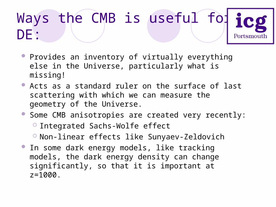
Ways the CMB is useful for DE: Provides an inventory of virtually everything else in

the Universe, particularly what is missing! Acts as a standard ruler on the surface of last

scattering with which we can measure the geometry of the Universe.

Some CMB anisotropies are created very recently: Integrated Sachs-Wolfe effect Non-linear effects like Sunyaev-Zeldovich

In some dark energy models, like tracking models, the dark energy density can change significantly, so that it is important at z=1000.

CMB as cosmic yardstick

WMAP compilationThe CMB is imprinted with the scale of the sound horizon at last scattering.

Both the curvature and the dark energy can change the angular size of the Doppler peaks. Assuming a cosmological constant, we get a constraint on curvature.

However, if we assume a flat universe, we can find a constraint on the equation of state.

Angular distance to last scattering surface

Ways the CMB is useful for DE: Provides an inventory of virtually everything else in

the Universe. Acts as a standard ruler on the surface of last

scattering with which we can measure the geometry of the Universe.

Some CMB anisotropies are created very recently: Integrated Sachs-Wolfe (ISW) effect Non-linear effects like Sunyaev-Zeldovich

In some dark energy models, like tracking models, the dark energy density can change significantly, so that it is important at z=1000.

Outline

What is the ISW effect?

Why is it interesting?

Detecting the ISW Examples

X-ray background SDSS quasars

Present limits Future measurements

Improving the detections

Conclusions

Two independent CMB maps

Late ISW map, z< 4 Mostly large scale features Requires dark energy/curvature

Early map, z~1000 Structure on many scales Sound horizon as yardstick

The CMB fluctuations we see are a combination of two largely uncorrelated pieces, one induced at low redshifts by a late time transition in the total equation of state.

Dark energy signature

The ISW effect is gravitational, much like gravitational lensing, but instead of probing the gravitational potential directly, it measures its time dependence along the line of sight.

gravitational potential traced by galaxy density

potential depth changes as cmb photons pass through

The gravitational potential is actually constant in a matter dominated universe on large scales. However, when the equation of state changes, so does the potential, and temperature anisotropies are created.

What can the ISW do for us?Differential measurement of structure evolution

Only arises when matter domination ends!

Independent evidence for dark energy Matter dominated universe in trouble

Direct probe of the evolution of structures Do the gravitational potentials grow or decay? Constrain modified gravity models?

Structure formation on the largest scales Measure dark energy clustering (Bean & Dore, Weller & Lewis, Hu & Scranton)

Modified gravity

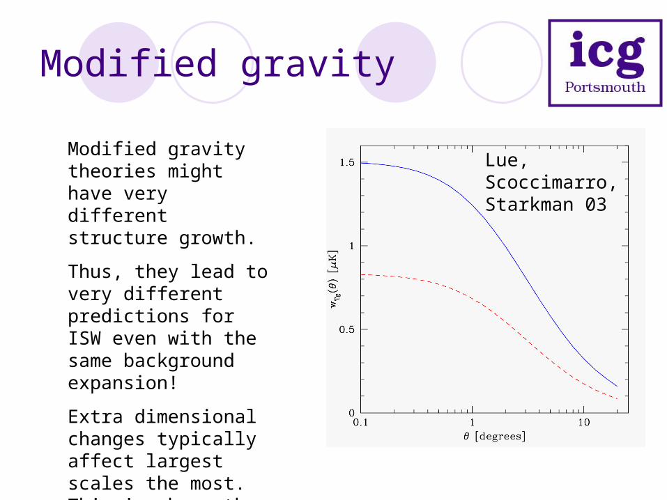
Lue, Scoccimarro, Starkman 03

Modified gravity theories might have very different structure growth.

Thus, they lead to very different predictions for ISW even with the same background expansion!

Extra dimensional changes typically affect largest scales the most. This is where the predictions are most uncertain.

DGP model

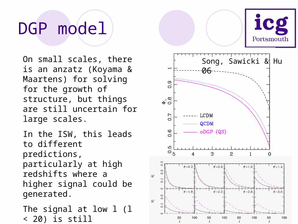
On small scales, there is an anzatz (Koyama & Maartens) for solving for the growth of structure, but things are still uncertain for large scales.

In the ISW, this leads to different predictions, particularly at high redshifts where a higher signal could be generated.

The signal at low l (l < 20) is still uncertain, though a new anzatz has recently been proposed. (Song, Sawicki & Hu).

Song, Sawicki & Hu 06

What can the ISW do for us?Differential measurement of structure evolution

Only arises when matter domination ends!

Independent evidence for dark energy Matter dominated universe in trouble

Direct probe of the evolution of structures Do the gravitational potentials grow or decay? Constrain modified gravity models?

Structure formation on the largest scales Measure dark energy clustering Potentially discriminate d.e. sound speeds at 3(Bean & Dore, Weller & Lewis, Hu & Scranton)

How do we detect ISW map?

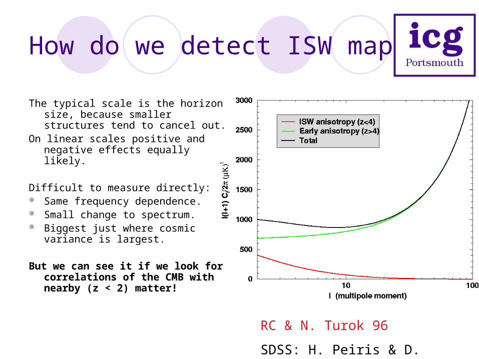
RC & N. Turok 96

SDSS: H. Peiris & D. Spergel 2000

The typical scale is the horizon size, because smaller structures tend to cancel out.

On linear scales positive and negative effects equally likely.

Difficult to measure directly: Same frequency dependence. Small change to spectrum. Biggest just where cosmic

variance is largest.

But we can see it if we look for correlations of the CMB with nearby (z < 2) matter!

Cross correlation spectrum

The gravitational potential determines where the galaxies form and where the ISW fluctuations are created!

Thus the galaxies and the CMB should be correlated, though its not a direct template.

Most of the cross correlation arises on large or intermediate angular scales (>1degree). The CMB is well determined on these scales by WMAP, but we need large galaxy surveys.

Can we observe this? Yes, but its difficult!

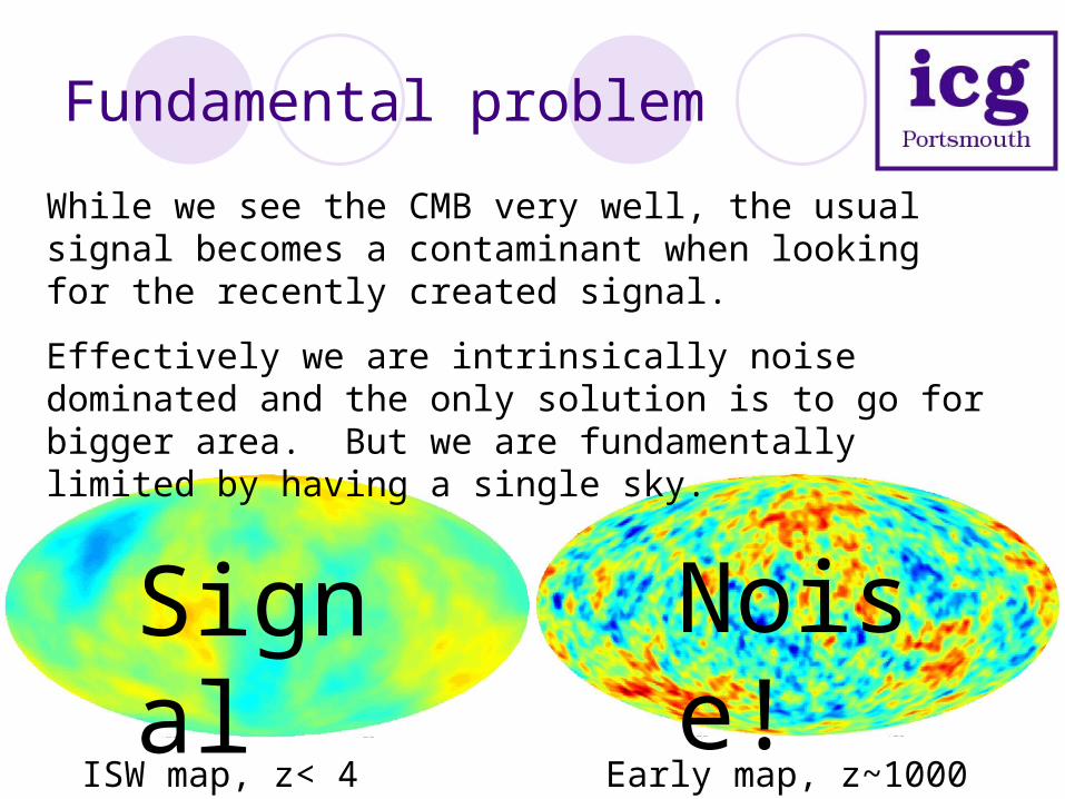
Fundamental problem

ISW map, z< 4 Early map, z~1000

While we see the CMB very well, the usual signal becomes a contaminant when looking for the recently created signal.

Effectively we are intrinsically noise dominated and the only solution is to go for bigger area. But we are fundamentally limited by having a single sky.

Noise!

Signal

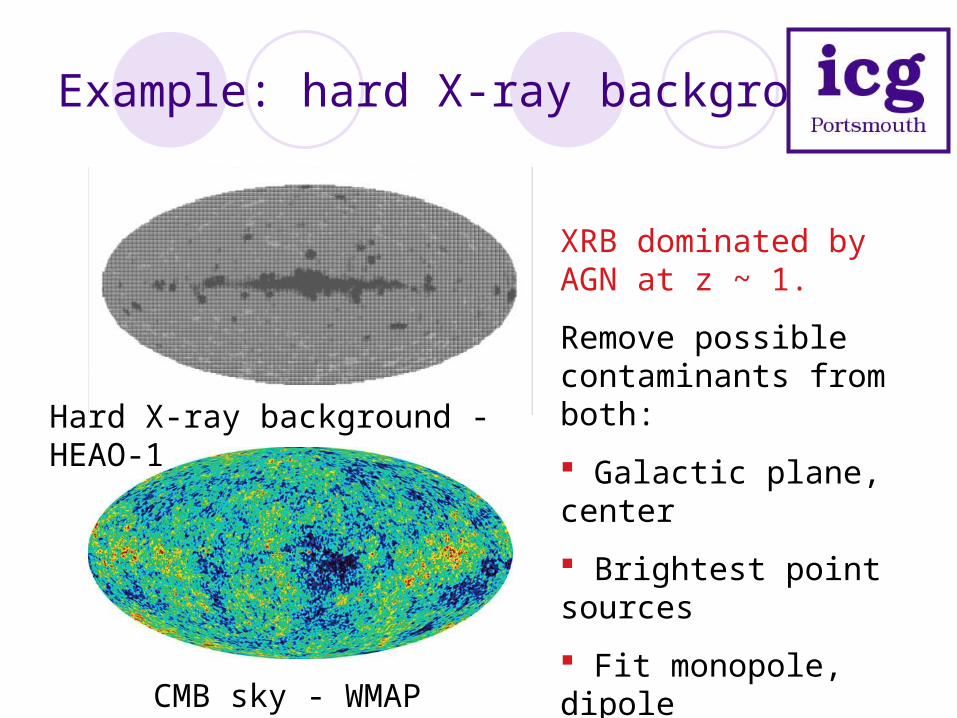
Example: hard X-ray background

Hard X-ray background - HEAO-1

CMB sky - WMAP

XRB dominated by AGN at z ~ 1.

Remove possible contaminants from both:

Galactic plane, center

Brightest point sources

Fit monopole, dipole

Detector time drifts

Local supercluster

Cross correlations observed!

What is the significance? Dominated not by measurement errors, but by possible accidental

alignments. This is modeled by correlating the XRB with random CMB maps with the

same spectrum. This gives the covariance matrix for the various bins.

Result: 3 detection

dots: observed

thin: Monte Carlos

thick: ISW prediction given best cosmology and dN/dz

errors highly correlated

S. Boughn & RC, 2004

Could it be a foreground?

Possible contaminations: Galactic foregrounds Clustered extra-galactic sources emitting in microwave Sunyaev-Zeldovich effect

Tests: • insensitive to level of galactic cuts• insensitive to point source cuts• comparable signal in both hemispheres• correlation on large angular scales• independent of CMB frequency channel

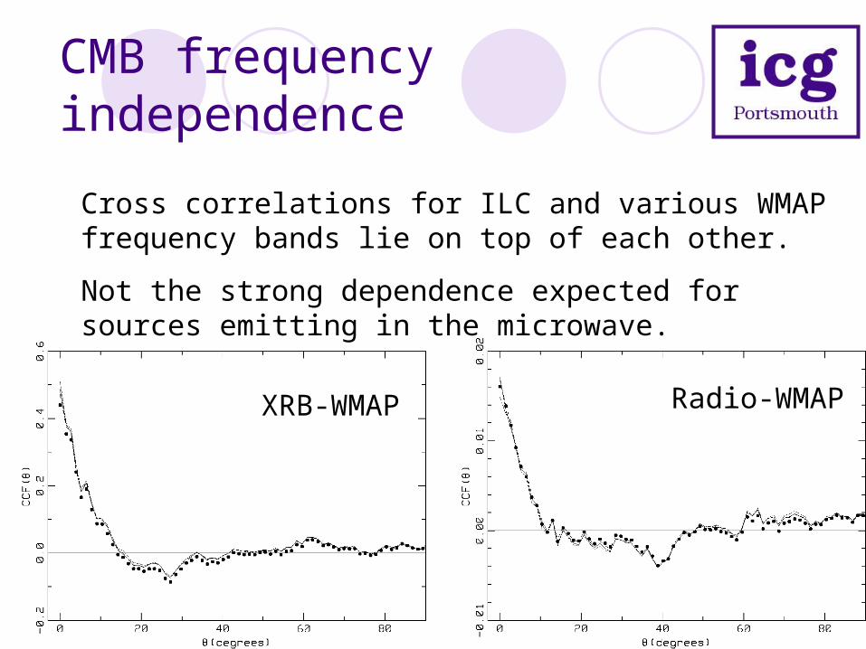
CMB frequency independence

Cross correlations for ILC and various WMAP frequency bands lie on top of each other.

Not the strong dependence expected for sources emitting in the microwave.

XRB-WMAP Radio-WMAP

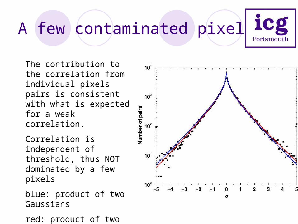
A few contaminated pixels?

The contribution to the correlation from individual pixels pairs is consistent with what is expected for a weak correlation.

Correlation is independent of threshold, thus NOT dominated by a few pixels

blue: product of two Gaussians

red: product of two weakly correlated Gaussians

Highest redshift detection of ISW To understand the evolution of the

potential, its important to push to higher redshifts.

One possible sample is the SDSS quasars (Peiris & Spergel 2000).

We use the photometrically selected sample of Richards et al. 2004

300,000 objects up to z =2.7. Covers 16% of the sky. Some fraction (~5%) are local stars that

are hard to distinguish in color space. Highest mean redshift of all ISW studies

so far; objects have individual redshifts!

T. Giannantonio, RC, R. Nichol et al - astro-ph/0607572

QSO map

We pixelize using HEALPIX, same as WMAP data.

We correct those edge pixels which are partially within the SDSS mask, weighting them less.

We explore the effects of potential systematics:

Dust extinction Poor seeing Bright sources Sky brightness

The largest effect is the extinction, so we cut out the 20% most reddened pixels.

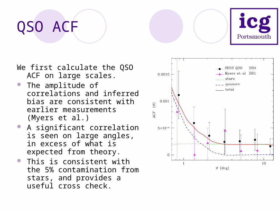
QSO ACF

We first calculate the QSO ACF on large scales.

The amplitude of correlations and inferred bias are consistent with earlier measurements (Myers et al.)

A significant correlation is seen on large angles, in excess of what is expected from theory.

This is consistent with the 5% contamination from stars, and provides a useful cross check.

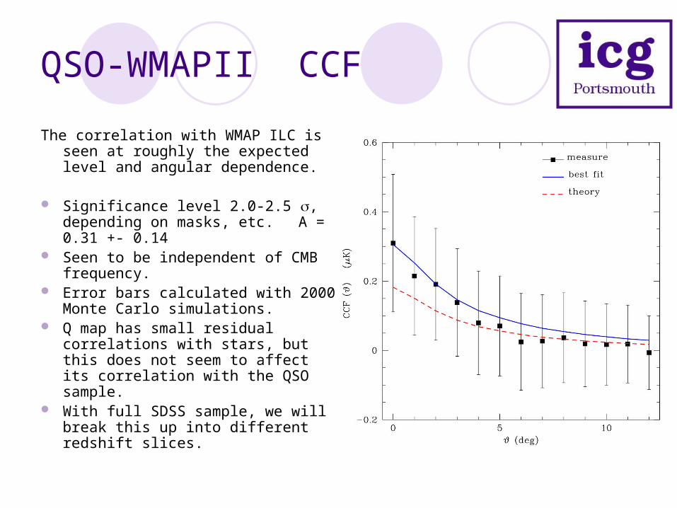
QSO-WMAPII CCF

The correlation with WMAP ILC is seen at roughly the expected level and angular dependence.

Significance level 2.0-2.5 ,

depending on masks, etc. A = 0.31 +- 0.14

Seen to be independent of CMB frequency.

Error bars calculated with 2000 Monte Carlo simulations.

Q map has small residual correlations with stars, but this does not seem to affect its correlation with the QSO sample.

With full SDSS sample, we will break this up into different redshift slices.

Correlations seen in many frequencies! X-ray background (Boughn & RC)

SDSS quasars (Giannantonio, RC, et al.)

Radio galaxies: NVSS confirmed by Nolta et al (WMAP collaboration)

Wavelet analysis shows even higher significance (Vielva et al. McEwan et al.)

FIRST radio galaxy survey (Boughn)

Infrared galaxies: 2MASS near infrared survey (Afshordi et al.)

Optical galaxies: APM survey (Folsalba & Gaztanaga)

Sloan Digital Sky Survey (Scranton et al., FGC, Cabre et al.)

Band power analysis of SDSS data (N. Pamanabhan, et al.)

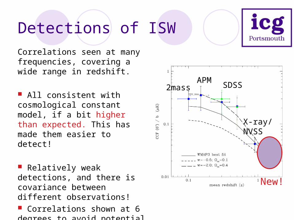
Detections of ISWCorrelations seen at many frequencies, covering a wide range in redshift.

All consistent with cosmological constant model, if a bit higher than expected. This has made them easier to detect!

Relatively weak detections, and there is covariance between different observations! Correlations shown at 6 degrees to avoid potential small angle contaminations (e.g. SZ). (Gaztanga et al.)

New!

2massAPM

SDSS

X-ray/NVSS

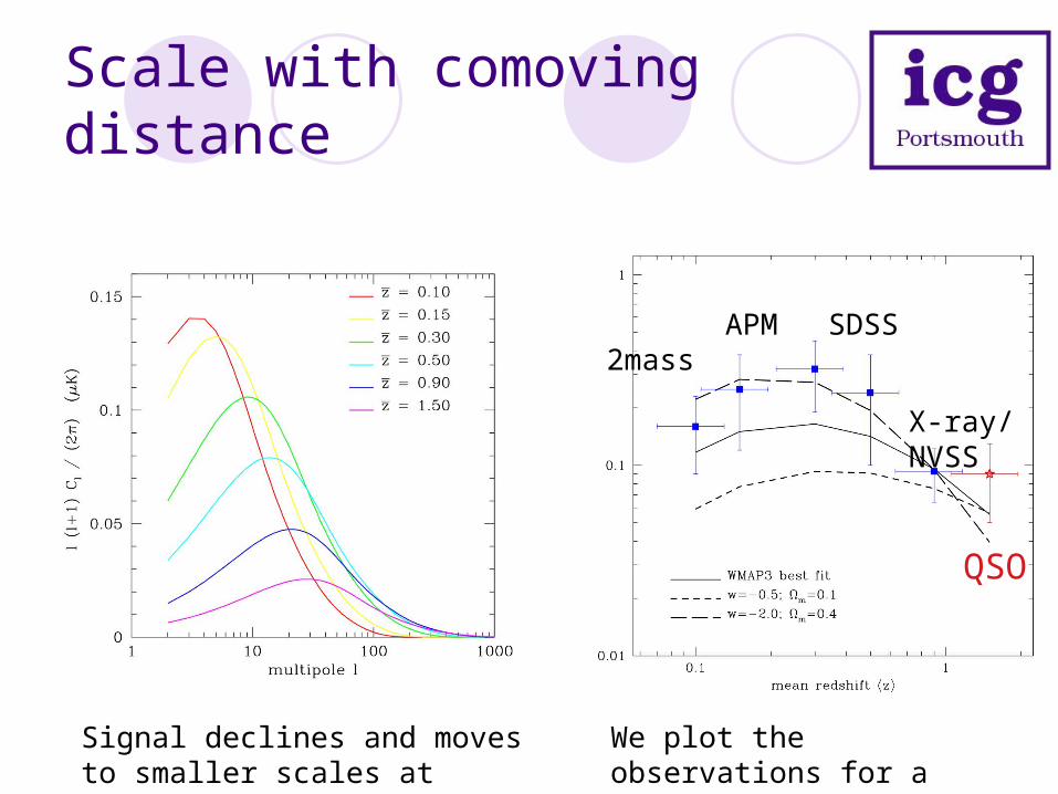
Scale with comoving distance

QSO

2massAPM SDSS

X-ray/NVSS

Signal declines and moves to smaller scales at higher redshift.

We plot the observations for a fixed projected distance.

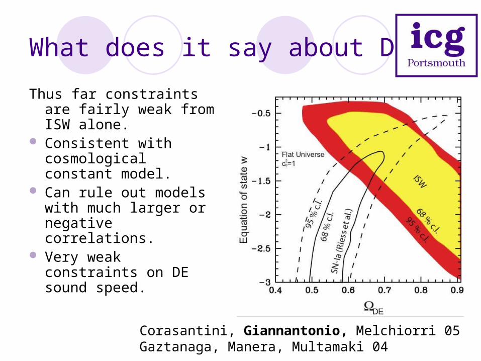
What does it say about DE?

Thus far constraints are fairly weak from ISW alone.

Consistent with cosmological constant model.

Can rule out models with much larger or negative correlations.

Very weak constraints on DE sound speed.

Corasantini, Giannantonio, Melchiorri 05Gaztanaga, Manera, Multamaki 04

Parameter constraints

A more careful job is needed!Quantify uncertainties: Bias - usually estimated from ACF consistently. How much

does it evolve over the samples? Non-linear or wavelength dependent?

Foregrounds - incorporate them into errors. dN/dz - how great are the uncertainties?

Understand errors: To use full angular correlations, we need full covariances for

all cross correlations. Monte Carlo’s needed with full cross correlations between

various surveys.

Extended covariance matrix

To combine them, we must understand whether and how the various experiments could be correlated:

Overlaps in sky coverage and redshift.

Magnification bias.

First efforts have begun to combine (Ryan Scranton & TG):

NVSS SDSS, LRG & QSO 2MASS

Preliminary results indicate > 5 total signal!

How good will it get?

This requires significant sky coverage, surveys with large numbers of galaxies and some understanding of the bias.

The contribution to (S/N)2 as a function of multipole moment.

This is proportional to the number of modes, or the fraction of sky covered, though this does depend on the geometry somewhat.

Of course, this assumes we have the right model-- It might be more! RC, N. Turok 96

Afshordi 2004

For the favoured cosmological constant the best signal to noise one can expect is about 7-10.

Future forecasts

Ideal experiment : Full sky, to overcome ‘noise’ 3-D survey, to weight in redshift (photo-z ok) z ~ 2-3, to see where DE starts 107 -108 galaxies, to beat Poisson noiseUnfortunately, z=1000 ‘noise’ limits the signal to the 7-10

level, even under the best conditions.Realistic plans: Short term - DES, Astro-F (AKARI) Long term - LSST, LOFAR/SKA

Pogosian et al 2005

astro-ph/ 0506396

Getting rid of the ‘noise’

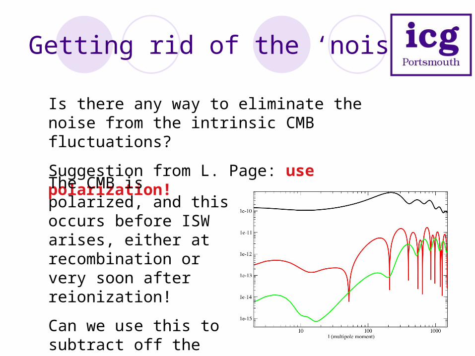
Is there any way to eliminate the noise from the intrinsic CMB fluctuations?

Suggestion from L. Page: use polarization!

The CMB is polarized, and this occurs before ISW arises, either at recombination or very soon after reionization!

Can we use this to subtract off the noise?

To some extent, yes!

The polarized temperature map

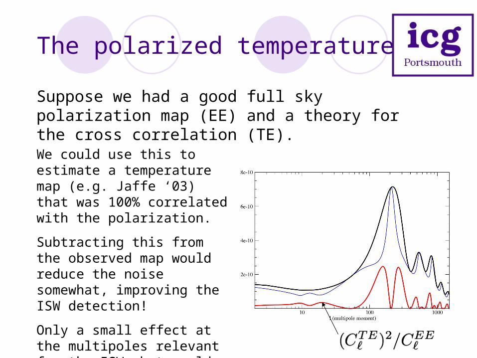
Suppose we had a good full sky polarization map (EE) and a theory for the cross correlation (TE).

We could use this to estimate a temperature map (e.g. Jaffe ‘03) that was 100% correlated with the polarization.

Subtracting this from the observed map would reduce the noise somewhat, improving the ISW detection!

Only a small effect at the multipoles relevant for the ISW, but could improve S/N by 20%.

Wavelet detections

Recent wavelet analyses (Vielva et al., McEwen et al) have apparently claimed better significance of detections than analyses using correlation functions.

NVSS-WMAP: CCFs give 2-2.5 ISW detections. Wavelets give 3.3-3.9 correlation detections. Despite better detection, parameter constraints comparable?!

What’s going on?

Claims:

Wavelets localize regions that correlate most strongly.

Better optimized for a single statistic than CCF(0).

Wavelet method

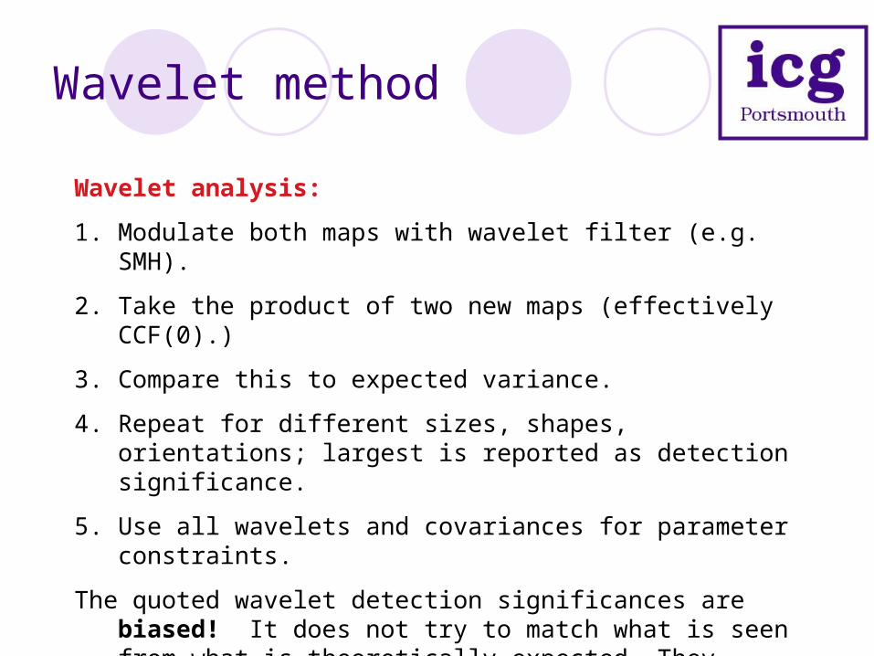
Wavelet analysis:

1. Modulate both maps with wavelet filter (e.g. SMH).

2. Take the product of two new maps (effectively CCF(0).)

3. Compare this to expected variance.

4. Repeat for different sizes, shapes, orientations; largest is reported as detection significance.

5. Use all wavelets and covariances for parameter constraints.

The quoted wavelet detection significances are biased! It does not try to match what is seen from what is theoretically expected. They actually present the probability of measuring precisely what they saw. The more wavelets they try, the better the more significant the detections will appear.

Wavelets vs correlation functions

Assuming the maps are Gaussian, the CCF or the power spectrum should be sufficient; they should contain all the information in the correlations.

It is true that wavelets do better for a single statistic, but CCF measurements look for particular angular dependence, combining different bins with full covariance.

In both cases, Gaussianity of quadratic statistics is assumed. The true full covariance distribution should be calculated to get true significance.

Wavelets could be improved by using information about the expected ISW signal, and the optimal ‘wavelet’ is simple to calculate, but it is not compact.

Conclusions

ISW effect is a useful cosmological probe, capable of telling us useful information about nature of dark energy.

It has been detected in a number of frequencies and a range of redshifts, providing independent confirmation of dark energy.

Many measurements are higher than expected, but what is the significance?

There is still much to do: Fully understanding uncertainties and covariances to do

best parameter estimation. Using full shape of probability distributions. Finding new data sets. Reducing ‘noise’ with polarization information.