DARK MATTER HALOS IN THE STANDARD COSMOLOGICAL MODEL ...hipacc.ucsc.edu/Bolshoi/images/Images/Klypin... · DARK MATTER HALOS IN THE STANDARD COSMOLOGICAL MODEL: RESULTS FROM THE BOLSHOI

The Astrophysical Journal, 740:102 (17pp), 2011 October 20 doi:10.1088/0004-637X/740/2/102C! 2011. The American Astronomical Society. All rights reserved. Printed in the U.S.A.

DARK MATTER HALOS IN THE STANDARD COSMOLOGICAL MODEL: RESULTS FROMTHE BOLSHOI SIMULATION

Anatoly A. Klypin1, Sebastian Trujillo-Gomez1, and Joel Primack21 Astronomy Department, New Mexico State University, Las Cruces, NM 880003-8001, USA

2 Department of Physics, University of California at Santa Cruz, Santa Cruz, CA, USAReceived 2010 March 12; accepted 2011 July 21; published 2011 October 4

ABSTRACT

Lambda Cold Dark Matter (!CDM) is now the standard theory of structure formation in the universe. We present thefirst results from the new Bolshoi dissipationless cosmological !CDM simulation that uses cosmological parametersfavored by current observations. The Bolshoi simulation was run in a volume 250 h"1 Mpc on a side using#8 billion particles with mass and force resolution adequate to follow subhalos down to the completeness limitof Vcirc = 50 km s"1 maximum circular velocity. Using merger trees derived from analysis of 180 stored timesteps we find the circular velocities of satellites before they fall into their host halos. Using excellent statistics ofhalos and subhalos (#10 million at every moment and #50 million over the whole history) we present accurateapproximations for statistics such as the halo mass function, the concentrations for distinct halos and subhalos,the abundance of halos as a function of their circular velocity, and the abundance and the spatial distribution ofsubhalos. We find that at high redshifts the concentration falls to a minimum value of about 4.0 and then risesfor higher values of halo mass—a new result. We present approximations for the velocity and mass functions ofdistinct halos as a function of redshift. We find that while the Sheth–Tormen (ST) approximation for the massfunction of halos found by spherical overdensity is quite accurate at low redshifts, the ST formula overpredicts theabundance of halos by nearly an order of magnitude by z = 10. We find that the number of subhalos scales withthe circular velocity of the host halo as V

1/2host , and that subhalos have nearly the same radial distribution as dark

matter particles at radii 0.3–2 times the host halo virial radius. The subhalo velocity function N (>Vsub) scales asV "3

circ. Combining the results of Bolshoi and Via Lactea-II simulations, we find that inside the virial radius of haloswith Vcirc = 200 km s"1 the number of satellites is N (>Vsub) = (Vsub/58 km s"1)"3 for satellite circular velocitiesin the range 4 km s"1 < Vsub < 150 km s"1.

Key words: cosmology: theory – large-scale structure of universe – methods: numerical

Online-only material: color figures

1. INTRODUCTION

The Lambda Cold Dark Matter (!CDM) model is the stan-dard modern theoretical framework for understanding the for-mation of structure in the universe (Dunkley et al. 2009). Withinitial conditions consisting of a nearly scale-free spectrum ofGaussian fluctuations as predicted by cosmic inflation, and withcosmological parameters determined from observations, !CDMmakes detailed predictions for the hierarchical gravitationalgrowth of structure. For the past several years, the best large sim-ulation for comparison with galaxy surveys has been the Millen-nium Simulation (MS-I; Springel et al. 2005). Here we presentthe first results from a new large cosmological simulation, whichwe are calling the Bolshoi simulation (“Bolshoi” is the Russianword for “big”3). Bolshoi has nearly an order of magnitude bet-ter mass and force resolution than the Millennium Run. TheMillennium Run used the first-year (WMAP1) cosmological pa-rameters from the Wilkinson Microwave Anisotropy Probe satel-lite (WMAP; Spergel et al. 2003). These parameters are nowknown to be inconsistent with modern measurements of thecosmological parameters. The Bolshoi simulation used the lat-est WMAP5 (Hinshaw et al. 2009; Komatsu et al. 2009; Dunkleyet al. 2009) and WMAP7 (Jarosik et al. 2011) parameters, whichare also consistent with other recent observational data.

The invention of CDM (Primack & Blumenthal 1984;Blumenthal et al. 1984) soon led to the first CDM N-body cos-

3 “Bolshoi” can be translated as (1) big or large, (2) great, (3) important, or(4) grown-up. The Bolshoi Ballet performs in Bolshoi Theater in Moscow.

mological simulations (Melott et al. 1983; Davis et al. 1985).Ever since then, such simulations have been essential in order tocalculate the predictions of CDM on scales where structure hasformed, since the nonlinear processes of structure formationcannot be fully described by analytic calculations. For exam-ple, one of the first large simulations of the !CDM cosmology(Klypin et al. 1996) showed that the dark matter autocorrelationfunction is much larger than the observed galaxy autocorrelationfunction on scales of #1 Mpc, so “scale-dependent anti-biasing”was required for !CDM to match the observed distribution ofgalaxies. Subsequent simulations with resolution adequate toidentify the dark matter halos that host galaxies (Jenkins et al.1998; Colın et al. 1999) demonstrated that the required destruc-tion of dark matter halos in dense regions does indeed occur.

N-body simulations have been essential for determining theproperties of dark matter halos. It turned out that dark matterhalos of all masses typically have a similar radial profile, whichcan be approximated by the Navarro–Frenk–White (NFW)profile (Navarro et al. 1996). Simulations were also crucial fordetermining the dependence of halo concentration cvir $ Rvir/rs

and halo shape on halo mass and redshift (Bullock et al. 2001;Zhao et al. 2003; Allgood et al. 2006; Neto et al. 2007; Maccioet al. 2008), and also for determining the dependence of theconcentration of halos on their mass accretion history (Wechsleret al. 2002; Zhao et al. 2009). Here, Rvir is the virial radiusand rs is the characteristic radius where the log–log slope ofthe density is equal to "2. Details are given in Section 3 andAppendix B.

1

http://dx.doi.org/10.1088/0004-637X/740/2/102

The Astrophysical Journal, 740:102 (17pp), 2011 October 20 Klypin, Trujillo-Gomez, & Primack

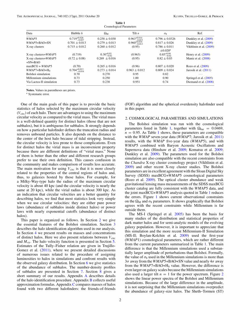
Table 1Cosmological Parameters

Data Hubble h "M Tilt n !8 Ref.

WMAP5 0.719+0.026"0.027 0.258 ± 0.030 0.963+0.014

"0.015 0.796 ± 0.0326 Dunkley et al. (2009)WMAP5+BAO+SN 0.701 ± 0.013 0.279 ± 0.013 0.960+0.014

"0.013 0.817 ± 0.026 Dunkley et al. (2009)X-ray clusters 0.715 ± 0.012 0.260 ± 0.012 (0.95) 0.786 ± 0.011 Vikhlinin et al. (2009)

±0.020a

X-ray clusters+WMAP5 (0.719) 0.30+0.03"0.02 (0.963) 0.85+0.04

"0.02 Henry et al. (2009)X-ray clusters+WMAP5 (0.72 ± 0.08) 0.269 ± 0.016 (0.95) 0.82 ± 0.03 Mantz et al. (2008)+SN+BAOmaxBCG + WMAP5 (0.70) 0.265 ± 0.016 (0.96) 0.807 ± 0.020 Rozo et al. (2009)WMAP7+BAO+H0 0.704+0.013

"0.014 0.273 ± 0.014 0.963 ± 0.012 0.809 ± 0.024 Jarosik et al. (2011)Bolshoi simulation 0.70 0.270 0.95 0.82 · · ·Millennium simulations 0.73 0.250 1.00 0.90 Springel et al. (2005)Via Lactea-II simulation 0.73 0.238 0.951 0.74 Diemand et al. (2008)

Notes. Values in parentheses are priors.a Systematic error.

One of the main goals of this paper is to provide the basicstatistics of halos selected by the maximum circular velocity(Vcirc) of each halo. There are advantages to using the maximumcircular velocity as compared to the virial mass. The virial massis a well-defined quantity for distinct halos (those that are notsubhalos), but it is ambiguous for subhalos. It strongly dependson how a particular halofinder defines the truncation radius andremoves unbound particles. It also depends on the distance tothe center of the host halo because of tidal stripping. Instead,the circular velocity is less prone to those complications. Evenfor distinct halos the virial mass is an inconvenient propertybecause there are different definitions of “virial mass.” Noneof them is better than the other and different research groupsprefer to use their own definition. This causes confusion inthe community and makes comparison of results less accurate.The main motivation for using Vcirc is that it is more closelyrelated to the properties of the central regions of halos and,thus, to galaxies hosted by those halos. For example, fora Milky-Way-type halo the radius of the maximum circularvelocity is about 40 kpc (and the circular velocity is nearly thesame at 20 kpc), while the virial radius is about 300 kpc. Asan indication that circular velocities are a better quantity fordescribing halos, we find that most statistics look very simplewhen we use circular velocities: they are either pure powerlaws (abundance of subhalos inside distinct halos) or powerlaws with nearly exponential cutoffs (abundance of distincthalos).

This paper is organized as follows. In Section 2 we givethe essential features of the Bolshoi simulation. Section 3describes the halo identification algorithm used in our analysis.In Section 4 we present results on masses and concentrationsof distinct halos. Here we also present relations between Vcircand Mvir. The halo velocity function is presented in Section 5.Estimates of the Tully–Fisher relation are given in Trujillo-Gomez et al. (2011), where we present detailed discussionsof numerous issues related to the procedure of assigningluminosities to halos in simulations and confront results withthe observed galaxy distribution. In Section 6 we give statisticsof the abundance of subhalos. The number-density profilesof subhalos are presented in Section 7. Section 8 gives ashort summary of our results. Appendix A describes detailsof the halo identification procedure. Appendix B collects usefulapproximation formulas. Appendix C compares masses of halosfound with two different halofinders: the friends-of-friends

(FOF) algorithm and the spherical overdensity halofinder usedin this paper.

2. COSMOLOGICAL PARAMETERS AND SIMULATIONSThe Bolshoi simulation was run with the cosmological

parameters listed in Table 1, together with "bar = 0.0469,n = 0.95. As Table 1 shows, these parameters are compatiblewith the WMAP seven-year data (WMAP7; Jarosik et al. 2011)results, with the WMAP five-year data (WMAP5), and withWMAP5 combined with Baryon Acoustic Oscillations andSupernova data (Hinshaw et al. 2009; Komatsu et al. 2009;Dunkley et al. 2009). The parameters used for the Bolshoisimulation are also compatible with the recent constraints fromthe Chandra X-ray cluster cosmology project (Vikhlinin et al.2009) and other recent X-ray cluster studies. The Bolshoiparameters are in excellent agreement with the Sloan Digital SkySurvey (SDSS) maxBCG+WMAP5 cosmological parameters(Rozo et al. 2009). The optical cluster abundance and weakgravitational lensing mass measurements of the SDSS maxBCGcluster catalog are fully consistent with the WMAP5 data, andthe joint maxBCG+WMAP5 analysis quoted in Table 1 reducesthe errors. Figure 1 shows current observational constraintson the "M and !8 parameters. It shows graphically that Bolshoiagrees with the recent constraints while Millennium is faroutside them.

The MS-I (Springel et al. 2005) has been the basis formany studies of the distribution and statistical properties ofdark matter halos and for semi-analytic models of the evolvinggalaxy population. However, it is important to appreciate thatthis simulation and the more recent Millennium-II Simulation(MS-II; Boylan-Kolchin et al. 2009) used the first-year(WMAP1) cosmological parameters, which are rather differentfrom the current parameters summarized in Table 1. The maindifference is that the Millennium simulations used a substan-tially larger amplitude of perturbations than Bolshoi. Formally,the value of !8 used in the Millennium simulations is more than3! away from the WMAP5+BAO+SN value and nearly 4! awayfrom the WMAP7+BAO+H0 value. However, the difference iseven larger on galaxy scales because the Millennium simulationsalso used a larger tilt n = 1 for the power spectrum. Figure 2shows the linear power spectra of the Bolshoi and Millenniumsimulations. Because of the large difference in the amplitude,it is not surprising that the Millennium simulations overpredictthe abundance of galaxy-size halos. The Sheth–Tormen (ST)

2


Figure 1. Optical and X-ray cluster abundance plus WMAP constraints on !8and "M . Contours show 68% confidence regions for a joint WMAP5 and clusterabundance analysis assuming a flat !CDM cosmology. The shaded region is theSDSS optical maxBCG cluster abundance + WMAP5 analysis from Rozo et al.(2009; which is also the source of this figure). The X-ray + WMAP5 constraintsare from several sources: the low-redshift cluster luminosity function (Mantzet al. 2008), the cluster temperature function (Henry et al. 2009), and the clustermass function (Vikhlinin et al. 2009). All four recent studies are in excellentagreement with each other and with the Bolshoi cosmological parameters. TheMillennium I and II cosmological parameters are far outside these constraints.

Figure 2. Bottom: linear power spectra of the Bolshoi and Millennium simu-lations at redshift zero. Top: ratio of the spectra. The Millennium simulationshave substantially larger amplitude of perturbations on all scales, resulting inoverprediction of the number of galaxy-size halos at high redshifts.(A color version of this figure is available in the online journal.)

approximation (Sheth & Tormen 2002) gives a factor of 1.3–1.7more Mvir % 1012 h"1 M& halos at z = 2–3 for Millenniumas compared with Bolshoi, which is a large difference. Angulo& White (2010) argue that cosmological N-body simulationscan be rescaled by certain approximations or by other means.However, the accuracy of those rescalings cannot be estimatedwithout running accurate simulations and testing particular char-acteristics.

Table 2Parameters of the Bolshoi Simulation

Parameter Value

Box size ( h"1 Mpc) 250Number of particles 20483

Mass resolution ( h"1 M&) 1.35 ' 108

Force resolution( h"1 kpc, physical) 1.0Initial redshift 80Zero-level mesh 2563

Maximum number ofrefinement levels 10Zero-level time step #a (2–3) ' 10"3

Maximum number of time steps #400,000Maximum displacement 0.10per time step (cell units)

The Bolshoi simulation uses a computational box250 h"1 Mpc across and 20483 % 8 billion particles, whichgives a mass resolution (one particle mass) of m1 = 1.35 '108 h"1 M&. The force resolution (smallest cell size) is a phys-ical (proper) 1 h"1 kpc (see below for details). For comparison,the MS-I had a force resolution (Plummer softening length)of 5 h"1 kpc and the MS-II had 1 h"1 kpc. Table 2 gives ashort summary of various numerical parameters of the Bolshoisimulation.

The Bolshoi simulation was performed with the Adaptive-Refinement-Tree (ART) code, which is an Adaptive-Mesh-Refinement (AMR)-type code. A detailed description of thecode is given in Kravtsov et al. (1997) and Kravtsov (1999). Thecode was parallelized using Massage Passing Interface (MPI)libraries and OpenMP directives (Gottloeber & Klypin 2008).Details of the time-stepping algorithm and comparison withGADGET and PKDGRAV codes are given in Klypin et al.(2009). Here we give a short outline of the code and presentdetails specific for Bolshoi.

The ART code starts with a homogeneous mesh covering thewhole cubic computational domain. For Bolshoi we use a 2563

mesh. The Cloud-In-Cell (CIC) method is used to obtain thedensity on the mesh. The Poisson equation is solved on the meshwith the fast Fourier transform method with periodic boundaryconditions. The ART code increases the force resolution bysplitting individual cubic cells into 2 ' 2 ' 2 cells with eachnew cell having half the size of its parent. This is done for everycell if the density of the cell exceeds some specified threshold.The value of the threshold varies with the level of refinementand with the redshift. Once the hierarchy of refinement cells isconstructed, the Poisson equation is solved on each refinementlevel using the Successive Over Relaxation technique withred–black alternations. Boundary conditions are taken from theone-level coarser grid. The initial guess for the gravitationalpotential is taken from the previous time step whenever possible.

We use the online Code for Anisotropies in the MicrowaveBackground of Lewis et al. (CAMB; 2000)4 to generate thepower spectrum of cosmological perturbations. The code isbased on the CMBFAST code by Seljak & Zaldarriaga (1996).

At early moments of evolution, when the amplitude of pertur-bations was small, the refinement thresholds were chosen in away that allows unimpeded growth of even the shortest perturba-tions, with wavelengths close to the Nyquist frequency. Ideally,the distance between particles should be at least two cell sizes:

4 http://lambda.gsfc.nasa.gov/toolbox/tb_camb_form.cfm

3

http://lambda.gsfc.nasa.gov/toolbox/tb_camb_form.cfm


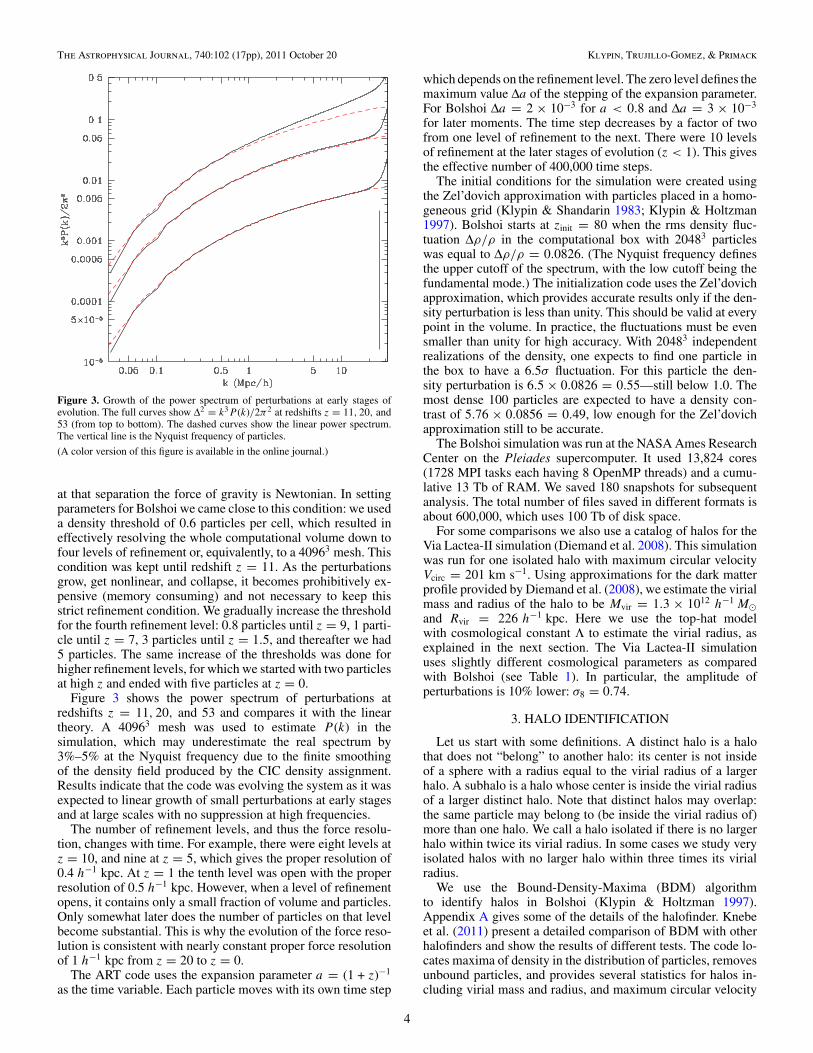
Figure 3. Growth of the power spectrum of perturbations at early stages ofevolution. The full curves show #2 = k3P (k)/2"2 at redshifts z = 11, 20, and53 (from top to bottom). The dashed curves show the linear power spectrum.The vertical line is the Nyquist frequency of particles.(A color version of this figure is available in the online journal.)

at that separation the force of gravity is Newtonian. In settingparameters for Bolshoi we came close to this condition: we useda density threshold of 0.6 particles per cell, which resulted ineffectively resolving the whole computational volume down tofour levels of refinement or, equivalently, to a 40963 mesh. Thiscondition was kept until redshift z = 11. As the perturbationsgrow, get nonlinear, and collapse, it becomes prohibitively ex-pensive (memory consuming) and not necessary to keep thisstrict refinement condition. We gradually increase the thresholdfor the fourth refinement level: 0.8 particles until z = 9, 1 parti-cle until z = 7, 3 particles until z = 1.5, and thereafter we had5 particles. The same increase of the thresholds was done forhigher refinement levels, for which we started with two particlesat high z and ended with five particles at z = 0.

Figure 3 shows the power spectrum of perturbations atredshifts z = 11, 20, and 53 and compares it with the lineartheory. A 40963 mesh was used to estimate P (k) in thesimulation, which may underestimate the real spectrum by3%–5% at the Nyquist frequency due to the finite smoothingof the density field produced by the CIC density assignment.Results indicate that the code was evolving the system as it wasexpected to linear growth of small perturbations at early stagesand at large scales with no suppression at high frequencies.

The number of refinement levels, and thus the force resolu-tion, changes with time. For example, there were eight levels atz = 10, and nine at z = 5, which gives the proper resolution of0.4 h"1 kpc. At z = 1 the tenth level was open with the properresolution of 0.5 h"1 kpc. However, when a level of refinementopens, it contains only a small fraction of volume and particles.Only somewhat later does the number of particles on that levelbecome substantial. This is why the evolution of the force reso-lution is consistent with nearly constant proper force resolutionof 1 h"1 kpc from z = 20 to z = 0.

The ART code uses the expansion parameter a = (1 + z)"1

as the time variable. Each particle moves with its own time step

which depends on the refinement level. The zero level defines themaximum value #a of the stepping of the expansion parameter.For Bolshoi #a = 2 ' 10"3 for a < 0.8 and #a = 3 ' 10"3

for later moments. The time step decreases by a factor of twofrom one level of refinement to the next. There were 10 levelsof refinement at the later stages of evolution (z < 1). This givesthe effective number of 400,000 time steps.

The initial conditions for the simulation were created usingthe Zel’dovich approximation with particles placed in a homo-geneous grid (Klypin & Shandarin 1983; Klypin & Holtzman1997). Bolshoi starts at zinit = 80 when the rms density fluc-tuation ##/# in the computational box with 20483 particleswas equal to ##/# = 0.0826. (The Nyquist frequency definesthe upper cutoff of the spectrum, with the low cutoff being thefundamental mode.) The initialization code uses the Zel’dovichapproximation, which provides accurate results only if the den-sity perturbation is less than unity. This should be valid at everypoint in the volume. In practice, the fluctuations must be evensmaller than unity for high accuracy. With 20483 independentrealizations of the density, one expects to find one particle inthe box to have a 6.5! fluctuation. For this particle the den-sity perturbation is 6.5 ' 0.0826 = 0.55—still below 1.0. Themost dense 100 particles are expected to have a density con-trast of 5.76 ' 0.0856 = 0.49, low enough for the Zel’dovichapproximation still to be accurate.

The Bolshoi simulation was run at the NASA Ames ResearchCenter on the Pleiades supercomputer. It used 13,824 cores(1728 MPI tasks each having 8 OpenMP threads) and a cumu-lative 13 Tb of RAM. We saved 180 snapshots for subsequentanalysis. The total number of files saved in different formats isabout 600,000, which uses 100 Tb of disk space.

For some comparisons we also use a catalog of halos for theVia Lactea-II simulation (Diemand et al. 2008). This simulationwas run for one isolated halo with maximum circular velocityVcirc = 201 km s"1. Using approximations for the dark matterprofile provided by Diemand et al. (2008), we estimate the virialmass and radius of the halo to be Mvir = 1.3 ' 1012 h"1 M&and Rvir = 226 h"1 kpc. Here we use the top-hat modelwith cosmological constant ! to estimate the virial radius, asexplained in the next section. The Via Lactea-II simulationuses slightly different cosmological parameters as comparedwith Bolshoi (see Table 1). In particular, the amplitude ofperturbations is 10% lower: !8 = 0.74.

3. HALO IDENTIFICATION

Let us start with some definitions. A distinct halo is a halothat does not “belong” to another halo: its center is not insideof a sphere with a radius equal to the virial radius of a largerhalo. A subhalo is a halo whose center is inside the virial radiusof a larger distinct halo. Note that distinct halos may overlap:the same particle may belong to (be inside the virial radius of)more than one halo. We call a halo isolated if there is no largerhalo within twice its virial radius. In some cases we study veryisolated halos with no larger halo within three times its virialradius.

We use the Bound-Density-Maxima (BDM) algorithmto identify halos in Bolshoi (Klypin & Holtzman 1997).Appendix A gives some of the details of the halofinder. Knebeet al. (2011) present a detailed comparison of BDM with otherhalofinders and show the results of different tests. The code lo-cates maxima of density in the distribution of particles, removesunbound particles, and provides several statistics for halos in-cluding virial mass and radius, and maximum circular velocity

4


Figure 4. Dependence of maximum circular velocity Vcirc on halo mass for distinct halos at redshift z = 0 (left panel) and redshift z = 3 (right panel). The circularvelocity at any moment mostly scales as Vcirc ( Mvir

1/3. The figure shows deviations from this scaling law. The deviations are related with the halo concentration.Full curves on both plots show median Vcirc and dashed curves show 90% limits. Dots represent individual halos with large masses.(A color version of this figure is available in the online journal.)

Vcirc =!

GM(<r)r

"""max

. (1)

Throughout this paper we will use Vcirc and the term circularvelocity to mean maximum circular velocity over all radii r.When a halo evolves over time, its Vcirc may also evolve. Thisis especially important for subhalos, which can be significantlytidally stripped and can reduce their Vcirc over time. Thus, wedistinguish instantaneous Vcirc and the peak circular velocityover halo’s history.

We use the virial mass definition Mvir that follows from thetop-hat model in an expanding universe with a cosmologicalconstant. We define the virial radius Rvir of halos as the radiuswithin which the mean density is the virial overdensity timesthe mean universal matter density #m = "M#crit at that redshift.Thus, the virial mass is given by

Mvir $ 4"

3#vir#mR3

vir . (2)

For our set of cosmological parameters, at z = 0 the virial radiusRvir is defined as the radius of a sphere with overdensity of 360 ofthe average matter density. The overdensity limit changes withredshift and asymptotically goes to 178 for high z. Differentdefinitions are also found in the literature. For example, theoften used overdensity 200 relative to the critical density givesmass M200, which for Milky-Way-mass halos is about 1.2–1.3times smaller than Mvir. The exact relation depends on haloconcentration.

Overall, there are about 10 million halos in Bolshoi. Halocatalogs are complete for halos with Vcirc > 50 km s"1

(Mvir % 1.5 ' 1010 h"1 M&). We track the evolution of eachhalo in time using #180 stored snapshots. The time differencebetween consecutive snapshots is rather small: #(40–80) Myr.

4. HALO MASS AND CONCENTRATION FUNCTIONS

Throughout most of the paper we characterize halos usingtheir circular velocity. However, Vcirc tightly correlates withhalo mass, as demonstrated in Figure 4. For distinct halos withMvir = 1012–1014 h"1 M&, 90% of halos have their circularvelocities within 8% of the median value. Even 99% of halos arewithin only 15%–20%. The variations are substantially largerfor subhalos: 90% of subhalos with masses 1011–1013 h"1 M&lie within 20% of the median Vcirc. On average, the circularvelocity increases with mass. The Vcirc–Mvir relation depends onhalo concentration c(Mvir), and, thus, studying this relation givesus a way to estimate c(Mvir) without making fits to individualhalo profiles. Any halo mass profile can be parameterized asM(r) = M0f (r/r0), where M0 and r0 are parameters withmass and radius units and the function f (x) is dimensionless. Ifxmax is the dimensionless radius corresponding to the maximumcircular velocity, then we can write the following relationbetween the maximum circular velocity and the virial mass(Klypin et al. 2001):

Vcirc =#G

f (xmax)f (c)

c

xmax#1/3

$1/2

Mvir1/3, (3)

# = Mvir

Rvir3 = 4"

3#vir#cr"M, (4)

f (x) = ln(1 + x) " x

1 + x, (5)

c = Rvir

rs

, x = R

rs

, xmax = 2.15. (6)

Here, #vir is the overdensity limit that defines the virial radius;#cr and "M are the critical density and the contribution of

5


Figure 5. Evolution of concentration of distinct halos with redshift. The fullcurves and symbols show results of simulations. Analytical approximationsare shown as dashed curves. All the fits have the same functional form ofEquation (12) with two free parameters. At low redshifts the halo concentrationdecreases with increasing mass. However, the trend changes at high redshiftswhen the concentration is nearly flat and even has a tendency to slightly increasewith mass.(A color version of this figure is available in the online journal.)

matter to the average density of the universe, respectively.The first two equations are general relations for any densityprofile. Equations (5) and (6) are specific for NFW: rs is thecharacteristic radius of the NFW profile, which is the radius atwhich the logarithmic slope of the density is "2. At z = 0,for our cosmological model, #vir = 360 and "m = 0.27.Calculating the numerical factors in Equations (3)–(6) we getthe following relation between virial mass, circular velocity, andconcentration at z = 0:

Vcirc(Mvir) = 6.72 ' 10"3Mvir1/3)c)

ln(1 + c) " c/(1 + c), (7)

where mass Mvir is in units of h"1M&, circular velocity is inunits of km s"1. This relation gives us an opportunity to estimatehalo concentration directly for a given virial mass and circularvelocity.

Alternatively, one may skip the c(M) term and simply usepower-law approximations for the Vcirc–Mvir relation that give agood fit to numerical data.

For distinct halos:

Vcirc(Mvir) = 2.8 ' 10"2Mvir0.316, (8)

and for subhalos:

Vcirc(Msub) = 3.8 ' 10"2Msub0.305. (9)

Here velocities are in km s"1 and masses are in units of h"1 M&.Equations (3)–(6) can be considered as equations for halo

concentration: for a given z, Mvir, and Vcirc one can solvethem to find c. For quiet halos the result must be the sameas what one gets from fitting halo density profiles with the NFWapproximation: two independent parameters (in our case Mvirand Vcirc) uniquely define the density profile. However, by using

Table 3Parameters of Fit Equation (12) for Virial Halo Concentration

Redshift c0 M0/ h"1 M& cmin c(1012 h"1 M&)

0.0 9.60 · · · · · · 9.600.5 7.08 1.5 ' 1017 5.2 7.21.0 5.45 2.5 ' 1015 5.1 5.82.0 3.67 6.8 ' 1013 4.6 4.63.0 2.83 6.3 ' 1012 4.2 4.45.0 2.34 6.6 ' 1011 4.0 5.0

only two parameters, we are prone to fluctuations. In order toreduce the effects of fluctuations we apply Equations (3)–(6)to the median values of Vcirc for each mass bin. For each massbin with the average Mvir we find the median circular velocityVcirc(Mvir, z). We then solve Equations (3)–(6) and get medianhalo concentrations c(Mvir, z). One can also find concentrationfor each halo and then take the median—the result is the samebecause for a given mass the relation between c and Vcirc ismonotonic. This procedure minimizes effects of fluctuations andgives the median halo concentration for a given mass. Munoz-Cuartas et al. (2011) applied our method to their simulationsand reproduced results of direct density profile fitting. Pradaet al. (2011) state that this method recovers results of haloconcentrations c(M) in MS-I (Neto et al. 2007) with deviationsof less than 5% over the whole range of masses in the simulation.

Figure 5 shows the concentrations for redshifts z = 0–5. Forredshift zero we get the following approximation:

c(Mvir) = 9.60%

Mvir

1012 h"1 M&

&"0.075

(10)

for distinct halos. For subhalos we find

c(Msub) = 12%

Msub

1012 h"1 M&

&"0.12

. (11)

Subhalos are clearly more concentrated than distinct haloswith the same mass, which is likely caused by tidal stripping.The differences between subhalos and distinct halos on averageare not large: a 30% effect in halo concentration.

We also study the evolution of distinct halo concentrationwith redshift. Figure 5 shows the concentrations for redshiftsz = 0–5. Results can be approximated using the followingfunctions:

c(Mvir, z) = c0(z)%

Mvir

1012 h"1 M&

&"0.075

''

1 +%

Mvir

M0(z)

&0.26(

, (12)

where c0(z) and M0(z) are two free factors for each z. Table 3gives the parameters for this approximation at different redshifts.For convenience we also give the concentration for a virial mass1012 h"1 M& and the minimum value of concentration cmin. Thesimulation box for Bolshoi is not large enough to find whetherthere is a minimum concentration for z < 0.5. For these epochsthe table gives the value of concentration at 1015 h"1 M& aspredicted by the analytical fits.

The curves in Figure 5 look different for different redshifts.Typically the concentration declines with redshift and the shapeof the curves evolves. Another interesting result is that the high-z curves show that the halo concentration has an upturn: for

6


Figure 6. Evolution of halo concentration for halos with two masses indicatedon the plot. The dots show results of simulations. For the reference the dashedlines show a power-law decline c ( (1 + z)"1. Concentrations do not changeas fast as the law predicts. At low redshifts z < 2 the decline in concentrationis c ( $ (dot-dashed curves), where $ is the linear growth factor. At highredshifts the concentration flattens and then slightly increases with mass. Forboth masses the concentration reaches a minimum of cmin % 4–4.5, but theminimum happens at different redshifts for different masses. The full curves areanalytical fits with the functional form of Equation (13).(A color version of this figure is available in the online journal.)

the most massive halos the concentration increases with mass.In order to demonstrate this more clearly, we study in moredetail the evolution with redshift of the halo concentration forhalos with two masses: 3 ' 1011 h"1 M& and 3 ' 1012 h"1 M&.Note that the masses are the same at different redshifts. So,this is not the evolution of the same halos. Figure 6 shows theresults. Just as expected, in both cases at low redshifts the haloconcentration declines with redshift. The decline is not as steepas often assumed c ( (1+z)"1; it is significantly shallower evenat low z. For z < 2 a power-law approximation c ( $(z) is amuch better fit, where $(z) is the linear growth factor. It is alsoa better approximation because the evolution of concentrationshould be related to the growth of perturbations, not to theexpansion of the universe. At larger z the concentration flattensand slightly increases at z > 3. The upturn is barely visible forthe larger mass, but it is clearly seen for the 3 ' 1011 h"1 M&mass halos. These and other results show that the concentrationin the upturn does not increase above c % 5 though it maybe related with the finite box size of our simulation. There isalso an indication that there is an absolute minimum of theconcentration cmin % 4 at high redshifts. Relaxed halos5 show aslightly stronger upturn indicating that non-equilibrium effectsare not the prime explanation for the increasing of the haloconcentration.

The following analytical approximations provide fits forthe evolution of concentrations for fixed masses as shown in

5 Relaxed halos are defined as halos with offset parameter Xoff < 0.07 andwith spin parameter % < 0.1, where Xoff is the distance from the halo center toits center of mass in units of the virial radius.

Figure 6:

c(Mvir, z) = c(Mvir, 0)[$4/3(z) + &($"1(z) " 1)]; (13)

here, $(z) is the linear growth factor of fluctuations normalizedto be $(0) = 1 and & is a free parameter, which for the massespresented in the figure is & = 0.084 for M = 3 ' 1011 h"1 M&and & = 0.135 for 10 times more massive halos with M =3 ' 1012 h"1 M&.

It is interesting to compare these results with other simula-tions. Zhao et al. (2003, 2009) were the first to find that the con-centration flattens at large masses and at high redshifts. Theirestimates of the minimum concentration are compatible withour results. Figure 2 in Zhao et al. (2003) shows an upturn inconcentration at z = 4. However, the results were noisy andinconclusive: the text does not even mention it.

Maccio et al. (2008) present results that can be directlycompared with ours because they use the same definition ofthe virial radius and estimate masses within spherical regions.Their models named WMAP5 have parameters that are veryclose to those of Bolshoi. There is one potential issue withtheir simulations. Maccio et al. (2008) use a set of simulationswith each simulation having a small number of particles andeither a low resolution, if the box size is large, or very smallbox, if the resolution is small. For all the halos in theirsimulations the approximation for concentration is c(Mvir) =8.41(Mvir/1012 h"1 M&)"0.108. Bolshoi definitely gives moreconcentrated halos. The largest difference is for cluster-sizehalos. For Mvir = 1015 h"1 M& our results give c = 5.7 whileMaccio et al. (2008) predict c = 4.0—a 40% difference. Thedifference gets smaller for galaxy-size halos: 14% for Mvir =1012 h"1 M& and 2% for Mvir = 1010 h"1 M&. Comparingresults for relaxed halos we find that the disagreement issmaller. Munoz-Cuartas et al. (2011) give c(Mvir) = 9.8 forMvir = 1012 h"1 M& as compared with our results (also forrelaxed halos) of c(Mvir) = 10.1—a 3% difference. For clusterswith Mvir = 1015 h"1 M& the disagreement is 18%.

We can also compare our results with those of MS-I (Netoet al. 2007), although MS-I has different cosmological pa-rameters and a different power spectrum. Because the anal-ysis of MS-I was done for the overdensity 200, we alsomade halo catalogs for this definition of halos. Neto et al.(2007) give the following approximation for all halos: c200 =7.75(M200/1012 h"1 M&)"0.11. For halos in the Bolshoi sim-ulation c200 = 7.2(M200/1012 h"1 M&)"0.075. Thus, the MS-I c200 is 8% larger than the concentrations in Bolshoi forMvir = 1012 h"1 M&, with a small (#10%) difference for Mvir =1014–1015 h"1 M&. For Mvir = 1012 h"1 M& in the MS-II andAquarius simulations Boylan-Kolchin et al. (2010) give an evenlarger concentration of cvir = 12.9, which is 1.3 times largerthan what we get from Bolshoi. Most of the differences arelikely due to the larger amplitude of cosmological fluctuationsin MS simulations because of the combination of a larger !8 anda steeper spectrum of fluctuations.

The mass function of distinct halos is a classical cosmologicalresult (e.g., Warren et al. 2006; Reed et al. 2007, 2009; Tinkeret al. 2008; Maccio et al. 2008). Figure 7 presents the resultsfor the Bolshoi simulation together with the predictions of theSheth–Tormen (ST) approximation (Sheth & Tormen 2002; seealso Appendix B). We find that the ST approximation givesan accurate fit for z = 0 with the deviations less than 10%for masses ranging from Mvir = 5 ' 109 h"1 M& to Mvir =5 ' 1014 h"1 M&. However, the ST approximation overpredictsthe abundance of halos at higher redshifts. For example, at

7


Figure 7. Mass function of distinct halos at different redshifts (circles). Curvesshow the ST approximation, which provides a very accurate fit at z = 0, butoverpredicts the number of halos at higher redshifts.(A color version of this figure is available in the online journal.)

z = 6 for halos with Mvir % (1–10) ' 1011 h"1 M& the STapproximation gives a factor of 1.5 more halos as comparedwith the simulation. At redshift 10 the ST approximation givesa factor of 10 more halos than what we find in the simulation.

We introduce a simple correction factor which brings theanalytical predictions much closer to the results of simula-tions. We find that the ST approximation multiplied by thefollowing factor gives less than 10% deviations for masses5 ' 109 h"1 M& " 5 ' 1014 h"1 M& and redshifts z = 0–10:

F ($) = (5.501$)4

1 + (5.500$)4, (14)

where $ is the linear growth-rate factor normalized to unity atz = 0 (see Equation (B2)).

Our results are in good agreement with Tinker et al. (2008),who present the evolution of the mass function for z = 0–2.5 forhalos defined using the spherical overdensity method. At redshiftzero, their mass function for overdensity # = 200 relative to themean mass density is 20% above the ST approximation. Thisis expected because masses defined with spherical overdensity# = 200 are typically 10%–20% larger than virial masses,which are used in our paper. Results in Tinker et al. (2008)together with our work indicate that at higher redshifts the massfunction gets further and further below the ST approximation.In addition, the shape of the mass function in simulations getssteeper: there is a greater disagreement at larger masses. Tinkeret al. (2008) argue that this behavior indicates that the massfunction is not “universal”: it does not scale with the redshiftonly as a function of the amplitude of perturbations ! (M) onscale M (see Appendix B for definitions). Our results extend thistrend to redshifts at least as large as z = 10. Our results alsoqualitatively agree with Cohn & White (2008), who presentspherical overdensity halo masses at z = 10. They also findsubstantially lower mass functions as compared with the STapproximation, though the differences with the approximationare somewhat smaller than what we find.

These results are at odds with those obtained with the FOFmethod (e.g., Lukic et al. 2007; Reed et al. 2007, 2009; Cohn &White 2008). The FOF halo mass function scales very close tothe “universal” ! (M) behavior. The reason for the disagreementbetween spherical overdensity and FOF halo-finding methods islikely related to the fact that FOF has a tendency to link togetherstructures before they become a part of a virialized halo. Thishappens more often with the rare most massive halos, whichhave a tendency to be out of equilibrium and in the processof merging. As a result of this, FOF masses are artificiallyinflated. Cohn & White (2008) studied case-by-case some halosat z = 10 and conclude that in their simulations FOF assignedto halos almost twice as much mass. Comparison of the STpredictions with the Bolshoi results shown in Figure 7 points tothe difference of a factor of 2.5 in mass for z = 10. Because ofthe steep decline of the mass function, a factor of 2.5 increase inmass translates to a factor of 10 increase in the number densityof halos. This correction to the FOF masses must be takeninto account when making any estimates of the frequency ofappearance of high-z objects.

In Appendix C we also directly compare FOF masses withthose obtained with the BDM code. At z = 8.8 the FOF masseswith the linking parameter l = 0.20 were on average 1.4 timeslarger than the BDM masses. In addition, the spread of estimateswas very large with FOF in many cases giving three to fivetimes larger masses than BDM. Analysis of individual casesshows that this happens because FOF links large fragments offilaments, not just an occasional neighboring halo. The situationis different at z = 0. Here both BDM and FOF (l = 0.17) giveremarkably similar results, though some spread is still present(Tinker et al. 2008). We speculate that the difference in thebehavior at high and low z is related to the slope of the powerspectrum of perturbations probed by halos at different redshifts.

These differences between different definitions of masses andradii of halos indicate the inherent weakness of masses as haloproperties: in the absence of a well-defined physical processresponsible for halo formation, masses are defined somewhatarbitrarily. We know that halos do not form according to theoften used top-hat model. We also know that the virial radiusis ill-defined for non-isolated interacting objects. Nevertheless,we use one definition or another and we pay a price for thisvagueness. These uncertainties in masses also motivate us to useanother, much better defined quantity—the maximum circularvelocity.

5. HALO VELOCITY FUNCTION

The velocity function for distinct halos is shown in Figure 8.It declines very steeply with velocity. At small velocities thepower slope is "3 with an exponential cutoff at large velocities.We find that at all redshifts the cumulative velocity function canbe accurately approximated by the following expression:

n(>V ) = AV "3 exp%

"#

V

V0

$'&, (15)

where the parameters A, V0, and ' are functions of redshift. Forz = 0 we find

A = 1.82 ' 104( h"1 Mpc/ km s"1)"3,

' = 2.5, (16)V0 = 800 km s"1.

The evolution of the parameters should not directly depend onthe redshift, but on the amplitude of perturbations. Indeed, when

8


Figure 8. Velocity function of distinct halos at different redshifts. Left: symbols and curves show the cumulative velocity function of the Bolshoi simulation. Errorbars show Gaussian fluctuations. Right: we plot the product V 3n(>V ) of the cumulative velocity function and the circular velocity. Dotted curves show analyticalapproximations with the form given by V 3n(>V ) = A exp("[V/V0]'), which provide accurate fits to numerical results.(A color version of this figure is available in the online journal.)

Figure 9. Parameters of the velocity function at different amplitudes ofperturbations !8(z). Open circles show parameters found by fitting n(>V, z) atdifferent redshifts. The curves are power-law fits given by Equations (15)–(17).The top right panel shows the evolution of !8 with redshift as predicted by thelinear theory. Circles on the curve indicate the same moments as on the otherthree panels.

we plot the parameters as functions of !8(z) as predicted by thelinear theory at different redshifts, the functions are very close topower laws as demonstrated by Figure 9. We find the followingfits to the parameters:

A = 1.52 ' 104!"3/48 (z)(h"1Mpc/ km s"1)"3,

' = 1 + 2.15!4/38 (z), (17)

V0 = 3300! 2

8 (z)1 + 2.5! 2

8 (z)km s"1.

Figure 10. Velocity function of satellites compared with the velocity functionof distinct halos. The bottom panel shows the cumulative function of subhalos(bottom full curve) and distinct halos (top full curve). The circular velocity usedfor the plot is the peak over each halo’s history. The dashed curves are analyticalapproximations. The top panel shows the ratio of the number of subhalos anddistinct halos (full curve) and an analytical approximation for the ratio (dashedcurve).

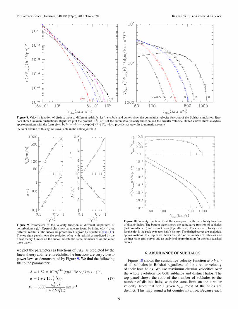
6. ABUNDANCE OF SUBHALOS

Figure 10 shows the cumulative velocity function n(>Vcirc)of all subhalos in Bolshoi regardless of the circular velocityof their host halos. We use maximum circular velocities overthe whole evolution for both subhalos and distinct halos. Thetop panel shows the ratio of the number of subhalos to thenumber of distinct halos with the same limit on the circularvelocity. Note that for a given Vcirc most of the halos aredistinct. This may sound a bit counter intuitive. Because each

9


Figure 11. Cumulative velocity function of satellites for host halos with differentmaximum circular velocities ranging from %150 km s"1 to %1000 km s"1 frombottom to top. The bottom panel uses the velocities of subhalos at redshift z = 0.The top panel uses peak circular velocities over the history of each subhalo. Thedashed lines show power laws with the slope "3. The abundance of subhalosincreases with increasing host halo mass.(A color version of this figure is available in the online journal.)

distinct halo has many subhalos, one would naively expectthat there are many more satellites as compared to distincthalos. This is not true. The number of satellites is large, butmost are small. When we count small distinct halos, theirnumber increases very fast and we always end up with moredistinct halos at a given circular velocity. The abundance ofsubhalos can be approximated with the same function given byEquation (15) as for the distinct halos. However, the parametersof the approximation are different. For subhalos that exist atz = 0 and for which we use peak velocities over their history ofevolution, we find

A = 6.2 ' 103( h"1 M&/ km s"1)"3

' = 2.2, V0 = 480 km s"1. (18)

The remarkable similarity of the shapes of the velocity functionsof halos and subhalos suggests a simple interpretation for thedifference in their parameters: subhalos were typically accretedat the epoch when the velocity function of distinct halos had thesame parameters ' and V0 as the velocity function of subhalosat present. For the parameters given by Equations (17) and (18)we get a typical accretion redshift, zacc % 1.

In order to study statistics of subhalos belonging to differentparent halos we split our sample of distinct halos into sub-samples with different ranges of circular velocities. For eachsubhalo we use either its z = 0 circular velocity or the peakvalue over its entire evolution. Figure 11 shows both the presentday and the peak velocity distribution functions for distincthalos with masses and velocities ranging from galaxy-size ha-los to clusters of galaxies. The average circular velocities foreach bin presented in the figure are (from bottom to top):Vhost = (163, 190, 235, 340, 470, 677, 936) km s"1. The num-ber of halos in each bin varies from 200 for the most massive

Figure 12. Dependence of the number of subhalos on the circular velocity oftheir hosts. Here we count all subhalos with circular velocities larger than 0.3 oftheir host circular velocity. The bottom panel shows results for Vcirc estimated atz = 0 and the top panel is for the peak Vcirc over the history of each subhalo. Forz = 0 circular velocities the abundance scales as V

1/2host (dashed curve). For peak

circular velocities the number of subhalos is larger and the scaling is steeper:N ( V

2/3host (full curve). For comparison, the dashed curve is the same as in the

bottom panel.(A color version of this figure is available in the online journal.)

halos (Vhost = 800–1200 km s"1) to 30,000 for the least mas-sive halos with Vhost = 160–180 km s"1. The increase in theabundance of substructure for more massive hosts is consis-tent with the results of Gao et al. (2004), who give a factor of2.0–2.5 increase for host halos from mass #2.5 ' 1012 h"1 M&to #1015 h"1 M&. Van den Bosch et al. (2005), Taylor & Babul(2005), and Zentner et al. (2005) came to similar conclusionsusing their (semi)analytic models.

In order to more accurately measure the dependence ofthe abundance of subhalos on the circular velocity of thehost halo, we analyze the number of satellites with circularvelocities larger than 0.3 of the circular velocity of their hosts:Vsat > 0.3Vhost. This approximately corresponds to the massratio of Msat/Mhost % 0.33 % 0.027. The threshold of 0.3 is acompromise between the statistics of satellites and the numericalresolution of the simulation. Figure 12 shows the number ofsatellites N0.3(Vhost) for hosts ranging from Vhost #150 km s"1

to #1000 km s"1. The number of satellites scales as a power-law N0.3 ( V

(host with the slope ( depending on how the circular

velocity is estimated. For the z = 0 velocities the slope is( = 1/2, and it is larger for the peak velocities: ( = 2/3.

There is an indication that the dependence of the cumulativenumber of satellites on their circular velocity N (>Vsat) getsslightly shallower for more massive host halos. Figure 13illustrates the point. Here we study the most massive (but alsorare) halos. Again, the number of satellites is approximatedby a power law. However, the slope is about "2.75, which issomewhat shallower than the slope of "3 found for smaller hosthalos.

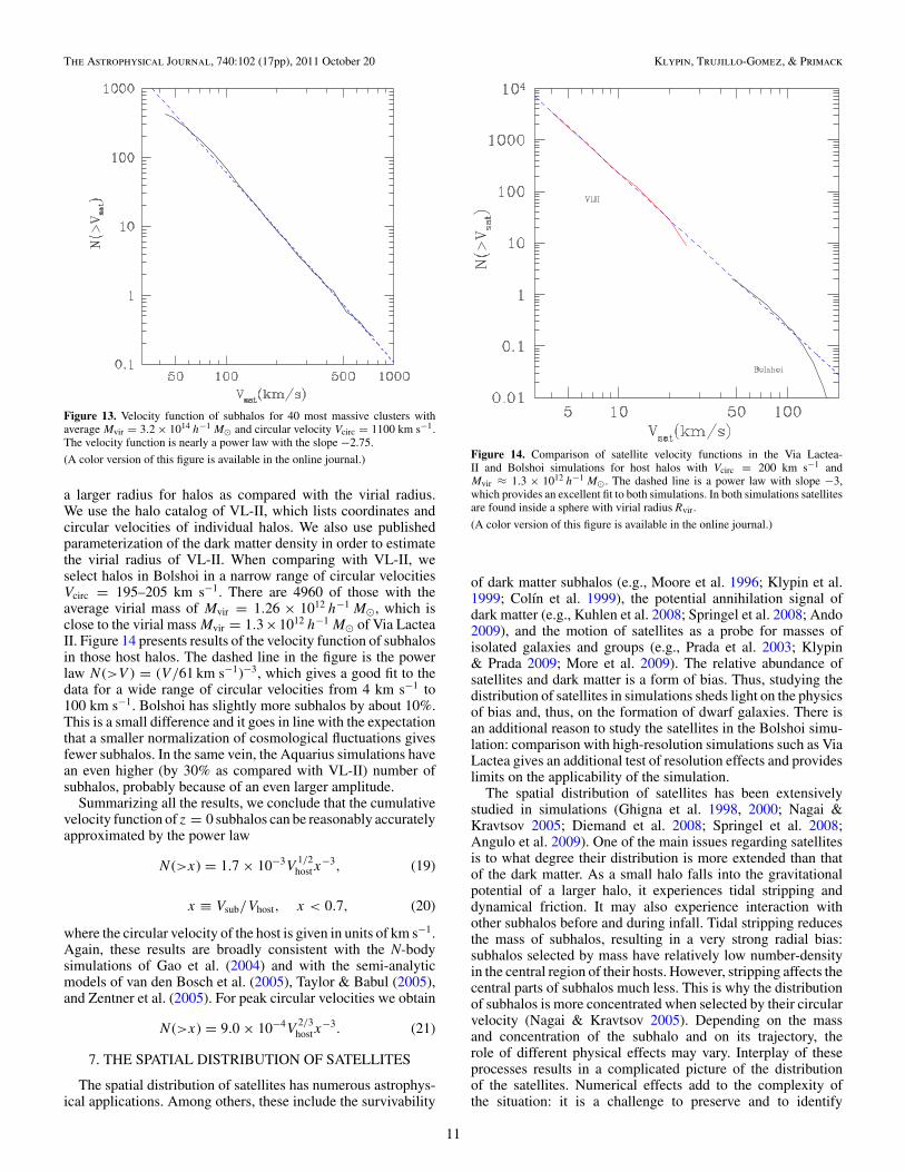
We compare some of our results with the Via Lactea-II(VL-II) simulation (Diemand et al. 2008). We do not use thepublished results because the analysis of VL-II was done usingoverdensity 180 relative to the matter density, which gives

10


Figure 13. Velocity function of subhalos for 40 most massive clusters withaverage Mvir = 3.2 ' 1014 h"1 M& and circular velocity Vcirc = 1100 km s"1.The velocity function is nearly a power law with the slope "2.75.(A color version of this figure is available in the online journal.)

a larger radius for halos as compared with the virial radius.We use the halo catalog of VL-II, which lists coordinates andcircular velocities of individual halos. We also use publishedparameterization of the dark matter density in order to estimatethe virial radius of VL-II. When comparing with VL-II, weselect halos in Bolshoi in a narrow range of circular velocitiesVcirc = 195–205 km s"1. There are 4960 of those with theaverage virial mass of Mvir = 1.26 ' 1012 h"1 M&, which isclose to the virial mass Mvir = 1.3'1012 h"1 M& of Via LacteaII. Figure 14 presents results of the velocity function of subhalosin those host halos. The dashed line in the figure is the powerlaw N (>V ) = (V/61 km s"1)"3, which gives a good fit to thedata for a wide range of circular velocities from 4 km s"1 to100 km s"1. Bolshoi has slightly more subhalos by about 10%.This is a small difference and it goes in line with the expectationthat a smaller normalization of cosmological fluctuations givesfewer subhalos. In the same vein, the Aquarius simulations havean even higher (by 30% as compared with VL-II) number ofsubhalos, probably because of an even larger amplitude.

Summarizing all the results, we conclude that the cumulativevelocity function of z = 0 subhalos can be reasonably accuratelyapproximated by the power law

N (>x) = 1.7 ' 10"3V1/2

hostx"3, (19)

x $ Vsub/Vhost, x < 0.7, (20)

where the circular velocity of the host is given in units of km s"1.Again, these results are broadly consistent with the N-bodysimulations of Gao et al. (2004) and with the semi-analyticmodels of van den Bosch et al. (2005), Taylor & Babul (2005),and Zentner et al. (2005). For peak circular velocities we obtain

N (>x) = 9.0 ' 10"4V2/3

hostx"3. (21)

7. THE SPATIAL DISTRIBUTION OF SATELLITES

The spatial distribution of satellites has numerous astrophys-ical applications. Among others, these include the survivability

Figure 14. Comparison of satellite velocity functions in the Via Lactea-II and Bolshoi simulations for host halos with Vcirc = 200 km s"1 andMvir % 1.3 ' 1012 h"1 M&. The dashed line is a power law with slope "3,which provides an excellent fit to both simulations. In both simulations satellitesare found inside a sphere with virial radius Rvir.(A color version of this figure is available in the online journal.)

of dark matter subhalos (e.g., Moore et al. 1996; Klypin et al.1999; Colın et al. 1999), the potential annihilation signal ofdark matter (e.g., Kuhlen et al. 2008; Springel et al. 2008; Ando2009), and the motion of satellites as a probe for masses ofisolated galaxies and groups (e.g., Prada et al. 2003; Klypin& Prada 2009; More et al. 2009). The relative abundance ofsatellites and dark matter is a form of bias. Thus, studying thedistribution of satellites in simulations sheds light on the physicsof bias and, thus, on the formation of dwarf galaxies. There isan additional reason to study the satellites in the Bolshoi simu-lation: comparison with high-resolution simulations such as ViaLactea gives an additional test of resolution effects and provideslimits on the applicability of the simulation.

The spatial distribution of satellites has been extensivelystudied in simulations (Ghigna et al. 1998, 2000; Nagai &Kravtsov 2005; Diemand et al. 2008; Springel et al. 2008;Angulo et al. 2009). One of the main issues regarding satellitesis to what degree their distribution is more extended than thatof the dark matter. As a small halo falls into the gravitationalpotential of a larger halo, it experiences tidal stripping anddynamical friction. It may also experience interaction withother subhalos before and during infall. Tidal stripping reducesthe mass of subhalos, resulting in a very strong radial bias:subhalos selected by mass have relatively low number-densityin the central region of their hosts. However, stripping affects thecentral parts of subhalos much less. This is why the distributionof subhalos is more concentrated when selected by their circularvelocity (Nagai & Kravtsov 2005). Depending on the massand concentration of the subhalo and on its trajectory, therole of different physical effects may vary. Interplay of theseprocesses results in a complicated picture of the distributionof the satellites. Numerical effects add to the complexity ofthe situation: it is a challenge to preserve and to identify

11


Figure 15. Density profiles for galaxy-size halos with Vcirc % 200 km s"1. Thefull curve and circles are the dark matter density and the number density ofsatellites with Vcirc > 4 km s"1 in the Via Lactea-II simulation normalized tothe average (number-)density for each component, respectively. The satelliteshave nearly the same overdensity as the dark matter for radii R = (0.3–2)Rvir.The number density of satellites falls below the dark matter at smaller radii. Thedashed curve is the number density of satellites with Vcirc > 80 km s"1 foundat z = 0 in the Bolshoi simulation for host halos selected to have the samecircular velocity as Via Lactea-II. In the outer regions with R = (0.5–1.5)Rvirthe satellites follow the dark matter very closely. In the inner regions the Bolshoiresults are 20%–30% below the much higher resolution simulation Via Lactea-II, presumably because of numerical effects.(A color version of this figure is available in the online journal.)

small subhalos throughout the whole history of evolution ofthe universe.

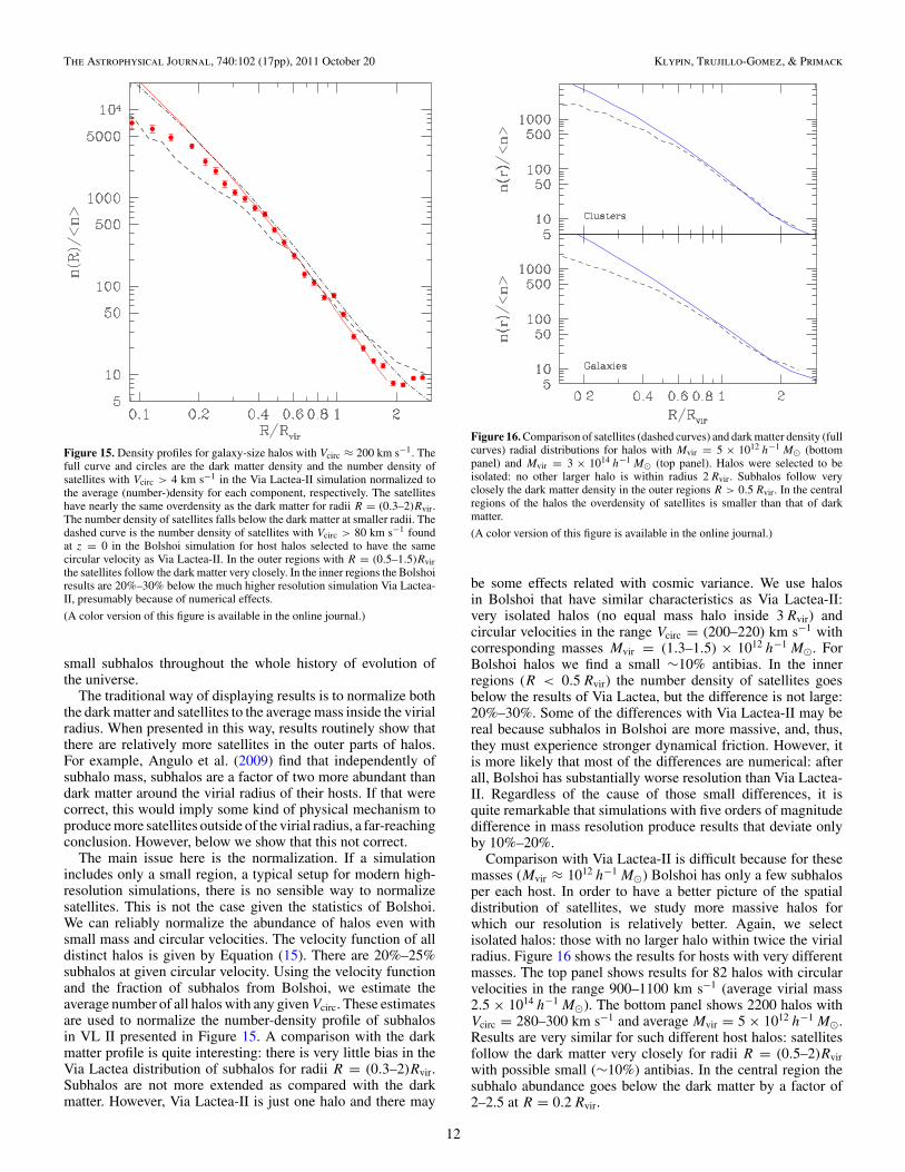
The traditional way of displaying results is to normalize boththe dark matter and satellites to the average mass inside the virialradius. When presented in this way, results routinely show thatthere are relatively more satellites in the outer parts of halos.For example, Angulo et al. (2009) find that independently ofsubhalo mass, subhalos are a factor of two more abundant thandark matter around the virial radius of their hosts. If that werecorrect, this would imply some kind of physical mechanism toproduce more satellites outside of the virial radius, a far-reachingconclusion. However, below we show that this not correct.

The main issue here is the normalization. If a simulationincludes only a small region, a typical setup for modern high-resolution simulations, there is no sensible way to normalizesatellites. This is not the case given the statistics of Bolshoi.We can reliably normalize the abundance of halos even withsmall mass and circular velocities. The velocity function of alldistinct halos is given by Equation (15). There are 20%–25%subhalos at given circular velocity. Using the velocity functionand the fraction of subhalos from Bolshoi, we estimate theaverage number of all halos with any given Vcirc. These estimatesare used to normalize the number-density profile of subhalosin VL II presented in Figure 15. A comparison with the darkmatter profile is quite interesting: there is very little bias in theVia Lactea distribution of subhalos for radii R = (0.3–2)Rvir.Subhalos are not more extended as compared with the darkmatter. However, Via Lactea-II is just one halo and there may

Figure 16. Comparison of satellites (dashed curves) and dark matter density (fullcurves) radial distributions for halos with Mvir = 5 ' 1012 h"1 M& (bottompanel) and Mvir = 3 ' 1014 h"1 M& (top panel). Halos were selected to beisolated: no other larger halo is within radius 2 Rvir. Subhalos follow veryclosely the dark matter density in the outer regions R > 0.5 Rvir. In the centralregions of the halos the overdensity of satellites is smaller than that of darkmatter.(A color version of this figure is available in the online journal.)

be some effects related with cosmic variance. We use halosin Bolshoi that have similar characteristics as Via Lactea-II:very isolated halos (no equal mass halo inside 3 Rvir) andcircular velocities in the range Vcirc = (200–220) km s"1 withcorresponding masses Mvir = (1.3–1.5) ' 1012 h"1 M&. ForBolshoi halos we find a small #10% antibias. In the innerregions (R < 0.5 Rvir) the number density of satellites goesbelow the results of Via Lactea, but the difference is not large:20%–30%. Some of the differences with Via Lactea-II may bereal because subhalos in Bolshoi are more massive, and, thus,they must experience stronger dynamical friction. However, itis more likely that most of the differences are numerical: afterall, Bolshoi has substantially worse resolution than Via Lactea-II. Regardless of the cause of those small differences, it isquite remarkable that simulations with five orders of magnitudedifference in mass resolution produce results that deviate onlyby 10%–20%.

Comparison with Via Lactea-II is difficult because for thesemasses (Mvir % 1012 h"1 M&) Bolshoi has only a few subhalosper each host. In order to have a better picture of the spatialdistribution of satellites, we study more massive halos forwhich our resolution is relatively better. Again, we selectisolated halos: those with no larger halo within twice the virialradius. Figure 16 shows the results for hosts with very differentmasses. The top panel shows results for 82 halos with circularvelocities in the range 900–1100 km s"1 (average virial mass2.5 ' 1014 h"1 M&). The bottom panel shows 2200 halos withVcirc = 280–300 km s"1 and average Mvir = 5 ' 1012 h"1 M&.Results are very similar for such different host halos: satellitesfollow the dark matter very closely for radii R = (0.5–2)Rvirwith possible small (#10%) antibias. In the central region thesubhalo abundance goes below the dark matter by a factor of2–2.5 at R = 0.2 Rvir.

12


It is interesting to compare the Bolshoi results with Nagai& Kravtsov (2005), who present profiles for eight clusters withalmost the same masses as in the top panel of our Figure 16. Ifwe change their normalization for subhalos selected by present-day circular velocity (their Figure 3) in such a way that the darkmatter profile matches the overdensity of satellites at the virialradius (we use a factor of 0.8 to match our definition of virialradius), then there is excellent agreement with Bolshoi, withboth simulations giving the ratio of the dark matter density tothe number density of satellites #2 at R = 0.2 Rvir.

8. CONCLUSIONS

Using the large halo statistics and high resolution of theBolshoi simulation we study numerous properties of halos andsubhalos. We present accurate analytical approximations forsuch characteristics as the halo and subhalo abundances andconcentrations, the velocity functions, and the number-densityprofiles of subhalos. Detailed discussions of different statisticshave already been given in relevant sections of the text. Here wepresent a short summary of our main conclusions.

Velocity function. Our main property of halos is their maxi-mum circular velocity Vcirc. As compared to virial masses, cir-cular velocities are better quantities for characterizing the phys-ical parameters of the central regions of dark matter halos. Assuch, they are better quantities for relating the dark matter ha-los and galaxies, which they host. We present the halo velocityfunctions at different redshifts and show that they can be ac-curately described by Equations (15)–(17). The halo circularvelocity function n(>V ) declines as a power-law V "3 at smallvelocities and has a quasi-exponential cutoff at large circularvelocities.

Mass function of distinct halos. We find that the ST approx-imation (Sheth & Tormen 2002) gives an accurate fit to theredshift-zero mass function: errors are less than 10% for massesin the range 5 ' 1010 h"1 M& " 5 ' 1014 h"1 M&. However,the approximation overpredicts the halo abundance at higherredshifts and gives a factor of 10 more halos than the Bolshoisimulation at z = 10. The correction factor Equation (14) bringsthe accuracy of the approximation back to the #10% level forredshifts z = 0"10. It also breaks the universality of the fit: themass function cannot be written as a function of only the rmsfluctuation ! (M) on mass scales M. These results depend onhow halos are defined with the FOF algorithm giving differentanswers than the spherical overdensity method. See Appendix Cfor details.

Concentrations of halos. The halo concentration c(Mvir, z)appears to be more complex than previously envisioned. For agiven redshift z, the concentration first declines with increasingmass. Then it flattens out and reaches a minimum of cmin % 4–5with the value of the minimum changing with redshift. At evenlarger masses c(Mvir) starts to slightly increase. This “upturn” inthe concentration is a weak feature: the change in concentrationis only 20%. Moreover, it cannot be detected at low redshifts,z < 0.5. If our estimates are correct, at z = 0 the upturnshould start at masses about Mvir # 1018 h"1 M&—clusters thismassive do not exist. However, at z > 2 the upturn is visibleat the very massive tail of the mass function. It is not clearwhat causes the upturn. The upturn is even stronger for relaxedhalos, which indicates that non-equilibrium effects cannot bethe reason for the upturn. At large redshifts the halos that showthe upturn are very rare: their mass is much larger than thecharacteristic mass M* of halos existing at that time. Most ofthem likely experience very fast growth. They also represent

very high-! peaks of the density field. It is known that thestatistics of rare peaks are different from those of more “normal”peaks (Bardeen et al. 1986). One may speculate that this mayresult in a change in halo concentration. More extensive analysisof halo concentrations is given in F. Prada et al. (2011, inpreparation).

Subhalo abundance. The cumulative abundance of satellitesis a power law with a steep slope: N (>V ) ( V "3. Combing ourresults with those of the Via Lactea-II simulation (Diemand et al.2008), we show that the power law extends at least from 4 km s"1

to 150 km s"1 for Milky-Way-mass halos and yields the correctabundance of large satellites such as the Large Magellanic Cloud(Busha et al. 2011). The abundance of satellites increases withthe circular velocity and mass of the host halo as N ( V

1/2host . For

example, this means that in relative units a cluster of galaxies has2.5 times more satellites than the Milky Way, in good agreementwith previous numerical results (Gao et al. 2004). Equations (20)and (21) give approximations for the abundance of satellites.

Subhalo number-density distribution. One of the main issueshere is the number density of satellites relative to the dark matterin the outer regions of halos. Some previous simulations indi-cated substantial (a factor of two) overabundance of satellitesaround the virial radius. We do not confirm this conclusion. Ourre-analysis of the Via Lactea-II simulation as well as the resultsfrom the Bolshoi simulation unambiguously show that there isno overabundance of satellites. In the Via Lactea-II simulationthe satellites follow very closely the distribution of dark matterfor radii R = (0.3–2)Rvir. In the Bolshoi simulation we find asmall (10%) antibias at the virial radius.

We thank F. Prada and A. Kravtsov for numerous helpfuldiscussions. We also thank S. Gottloeber for commenting onour paper and for allowing us to use his FOF halo catalog. Weare grateful to P. Madau and M. Kuhlen for providing us the halocatalog of the Via Lactea-II simulation and for discussions. Wethank M. Boylan-Kolchin for commenting on the abundanceof halos in the Millennium simulations. We thank the readerfor reading this long manuscript. We acknowledge support ofNSF grants to NMSU and NASA and NSF grants to UCSC.Our simulations and analysis were done at the NASA AmesResearch Center.

APPENDIX A

BOUND-DENSITY-MAXIMA HALOFINDER

We use a parallel (MPI+OpenMP) version of the Bound-Density-Maxima algorithm to identify halos in Bolshoi (Klypin& Holtzman 1997). For detailed comparison with other halofind-ers see Knebe et al. (2011). The code detects both distinct halosand subhalos. The code locates maxima of density in the dis-tribution of particles, removes unbound particles, and providesseveral statistics for halos including virial mass and radius, aswell as maximum circular velocity. The parameters of the BDMhalofinder were set such that the density maxima are not allowedto be closer than 10 h"1 kpc. We keep only the more massivedensity maximum6 if that happens. This is mostly done to savecomputer time. It is also consistent with the force resolutionof Bolshoi. Halo catalogs obtained with a smaller minimumseparation of 7.5 h"1 kpc did not include more halos.

6 We keep the peak that has the largest mass inside a sphere of radius10 h"1 kpc.

13


Removal of unbound particles is done iteratively. It goes insteps:

1. Find the bulk velocity of a halo: the velocity with whichthe halo moves in space. The rms velocities of individualparticles are later found relative to this velocity. We use thecentral region of the halo (the 30 particles closest to thehalo center) to find the bulk velocity.

2. Find the halo radius: the minimum of the virial radius andthe radius of the declining part of the density profile (radiusof the density minimum, if it exists).

3. Find the rms velocity of dark matter particles and thecircular velocity profile. Estimate the halo concentration.

4. Find the escape velocity as a function of radius and removeparticles that exceed the escape velocity. Use only boundparticles for the next iteration.

The whole procedure (steps 1–4) is repeated four times. Ifthe mass or radius of a halo is too small (too few particles), thedensity maximum is removed from the list of halo candidates.

If two halos (1) are separated by less than one virial radius, (2)have masses that differ by less than a factor of 1.5, and (3) havea relative velocity less than 0.15 of the rms velocity of darkmatter particles inside the halos, we remove the smaller haloand keep only the larger one. This is done to remove a defectof halo-finding where the same halo is identified more thanonce. This removal of “duplicates” (halos with nearly the samemass, position, and velocity) happens only during major mergerevents when instead of two merging nearly equal-mass halos thehalofinder sometimes finds three to five halos. Unfortunately,this also has the side effect of removing one of the major mergerhalos. This is a relatively rare event and it affects only the verytip of the subhalo velocity function.

We use the virial mass definition Mvir that follows from thetop-hat model in an expanding universe with a cosmologicalconstant. We define the virial radius Rvir of halos as the radiuswithin which the mean density is the virial overdensity timesthe mean universal matter density #m = "M#crit at that redshift.Thus, the virial mass is given by

Mvir $ 4"

3#vir#mR3

vir . (A1)

Equation (B1) gives an analytical approximation for #vir. Forour set of cosmological parameters, at z = 0 the virial radiusRvir is defined as the radius of a sphere with overdensity of 360times the average matter density. The overdensity limit changeswith redshift and asymptotically approaches 178 for high z.

Overall, there are about 10 million halos in Bolshoi (8.8M at z = 0, 12.3 M at z = 2, 4.8 M at z = 5). Halocatalogs are complete for halos with Vcirc > 50 km s"1

(Mvir % 1.5'1010 h"1 M&). We do post-processing of identifiedhalos. In particular, for distinct halos we find their properties(e.g., mass, circular velocity, density profiles) without removingunbound particles. For most, but not all, halos it makes littledifference. For example, the differences in circular velocitiesare less than a percent for halos with and without unboundparticles. Differences in mass can be a few percent dependingon halo mass and on environment.

In order to track the evolution of halos over time, we findand store the 50 most bound particles (fewer, if the halo doesnot have 50 particles). Together with other parameters of thehalo (coordinates, velocities, virial mass, and circular velocity)the information on most bound particles is used to identify thesame halos at different moments of time. The procedure of halo

Figure 17. Fraction of z = 0 halos tracked to a given redshift for halos withdifferent circular velocities at redshift zero.

tracking starts at z = 0 and goes back in time. The final result isthe history (track) of the major progenitor of a given halo. Thehalo track may be lost at some high redshift when the halo eitherbecomes too small to be detected or the tracking algorithm failsto find it. A new halo track may be initiated at some redshift ifthere is a halo for which there was no track at previous snapshots(smaller redshifts). This happens when a halo merges and getsabsorbed by another halo.

With #180 snapshots stored, the time difference betweenconsecutive snapshots is rather small. For example, the snapshotbefore the z = 0 snapshot has z = 0.0027 with a time differenceof 37 Myr. The difference in time between snapshots stayson nearly the same level (42–46 Myr) until z = 0.23 whenit becomes twice as large. We start with z = 0 halos andidentify them in the previous snapshot. If a halo is not foundat that snapshot, we try the next one. Altogether, we may trysix snapshots. Typically, 95% of halos are found in the previoussnapshot, an additional 2%–3% in the next one and #1% in evenearlier ones. Overall, about (0.2%–0.3)% of halos cannot betracked at any given snapshot: they are either lost because theirprogenitor gets too small or because of numerical problems. Thenumber depends on the redshift and on halo mass. Figure 17shows the fraction of halos tracked to given redshift for halosthat exist at z = 0. More massive halos are tracked to largerredshifts. Half of all halos with Vcirc = 50 km s"1 are tracked toz = 4 and half of all halos with Vcirc = 200 km s"1 are trackedto z = 7.

APPENDIX B

AUXILIARY APPROXIMATIONS

For completeness, here we present some approximations usedin the text. For the family of flat cosmologies ("M + "! = 1) anaccurate approximation for the value of the virial overdensity#vir is given by the analytic formula (Bryan & Norman 1998):

#vir = (18"2 + 82x " 39x2)/"(z), (B1)

where "(z) $ #m(z)/#crit and x $ "(z) " 1.

14


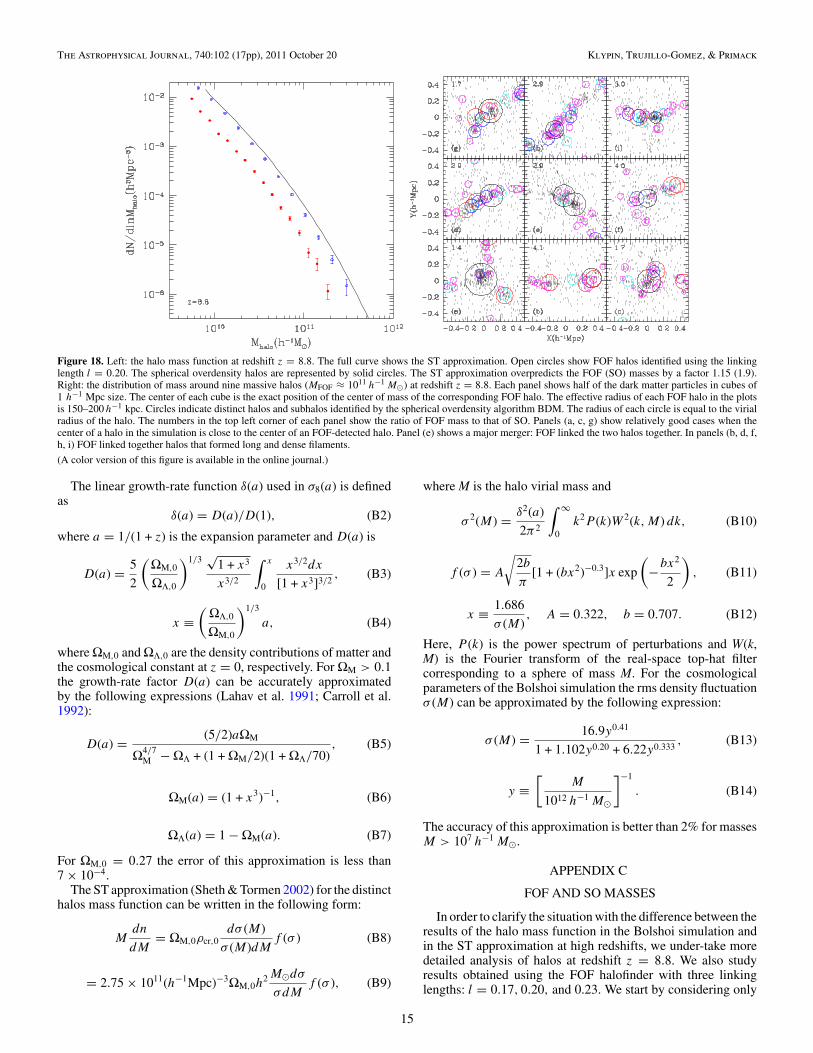
Figure 18. Left: the halo mass function at redshift z = 8.8. The full curve shows the ST approximation. Open circles show FOF halos identified using the linkinglength l = 0.20. The spherical overdensity halos are represented by solid circles. The ST approximation overpredicts the FOF (SO) masses by a factor 1.15 (1.9).Right: the distribution of mass around nine massive halos (MFOF % 1011 h"1 M&) at redshift z = 8.8. Each panel shows half of the dark matter particles in cubes of1 h"1 Mpc size. The center of each cube is the exact position of the center of mass of the corresponding FOF halo. The effective radius of each FOF halo in the plotsis 150–200 h"1 kpc. Circles indicate distinct halos and subhalos identified by the spherical overdensity algorithm BDM. The radius of each circle is equal to the virialradius of the halo. The numbers in the top left corner of each panel show the ratio of FOF mass to that of SO. Panels (a, c, g) show relatively good cases when thecenter of a halo in the simulation is close to the center of an FOF-detected halo. Panel (e) shows a major merger: FOF linked the two halos together. In panels (b, d, f,h, i) FOF linked together halos that formed long and dense filaments.(A color version of this figure is available in the online journal.)

The linear growth-rate function $(a) used in !8(a) is definedas

$(a) = D(a)/D(1), (B2)

where a = 1/(1 + z) is the expansion parameter and D(a) is

D(a) = 52

%"M,0

"!,0

&1/3 )1 + x3

x3/2

) x

0

x3/2dx

[1 + x3]3/2, (B3)

x $%

"!,0

"M,0

&1/3

a, (B4)

where "M,0 and "!,0 are the density contributions of matter andthe cosmological constant at z = 0, respectively. For "M > 0.1the growth-rate factor D(a) can be accurately approximatedby the following expressions (Lahav et al. 1991; Carroll et al.1992):

D(a) = (5/2)a"M

"4/7M " "! + (1 + "M/2)(1 + "!/70)

, (B5)

"M(a) = (1 + x3)"1, (B6)

"!(a) = 1 " "M(a). (B7)

For "M,0 = 0.27 the error of this approximation is less than7 ' 10"4.

The ST approximation (Sheth & Tormen 2002) for the distincthalos mass function can be written in the following form:

Mdn

dM= "M,0#cr,0

d! (M)! (M)dM

f (! ) (B8)

= 2.75 ' 1011(h"1Mpc)"3"M,0h2 M&d!

!dMf (! ), (B9)

where M is the halo virial mass and

! 2(M) = $2(a)2"2

) +

0k2P (k)W 2(k,M) dk, (B10)

f (! ) = A

!2b

"[1 + (bx2)"0.3]x exp

%"bx2

2

&, (B11)

x $ 1.686! (M)

, A = 0.322, b = 0.707. (B12)

Here, P (k) is the power spectrum of perturbations and W(k,M) is the Fourier transform of the real-space top-hat filtercorresponding to a sphere of mass M. For the cosmologicalparameters of the Bolshoi simulation the rms density fluctuation! (M) can be approximated by the following expression:

! (M) = 16.9y0.41

1 + 1.102y0.20 + 6.22y0.333, (B13)

y $#

M

1012 h"1 M&

$"1

. (B14)

The accuracy of this approximation is better than 2% for massesM > 107 h"1 M&.

APPENDIX C

FOF AND SO MASSES

In order to clarify the situation with the difference between theresults of the halo mass function in the Bolshoi simulation andin the ST approximation at high redshifts, we under-take moredetailed analysis of halos at redshift z = 8.8. We also studyresults obtained using the FOF halofinder with three linkinglengths: l = 0.17, 0.20, and 0.23. We start by considering only

15


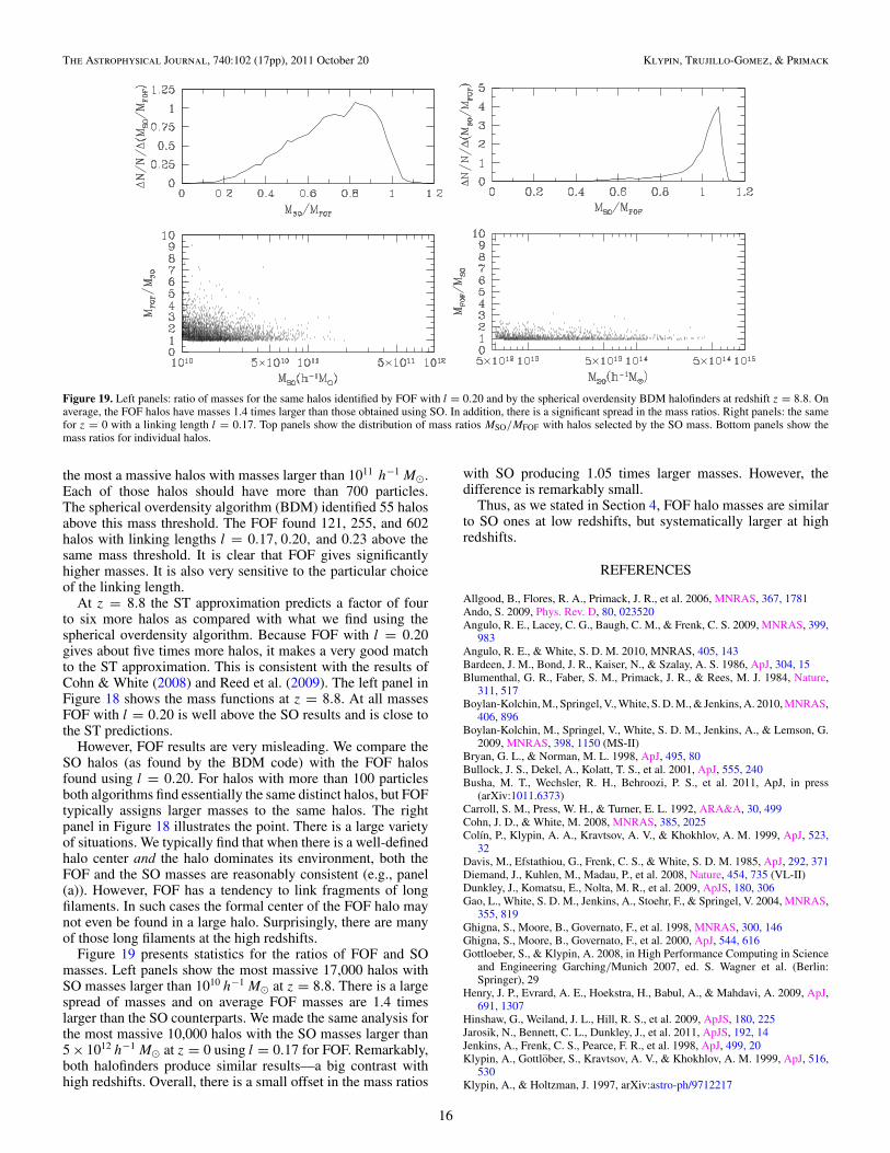
Figure 19. Left panels: ratio of masses for the same halos identified by FOF with l = 0.20 and by the spherical overdensity BDM halofinders at redshift z = 8.8. Onaverage, the FOF halos have masses 1.4 times larger than those obtained using SO. In addition, there is a significant spread in the mass ratios. Right panels: the samefor z = 0 with a linking length l = 0.17. Top panels show the distribution of mass ratios MSO/MFOF with halos selected by the SO mass. Bottom panels show themass ratios for individual halos.

the most a massive halos with masses larger than 1011 h"1 M&.Each of those halos should have more than 700 particles.The spherical overdensity algorithm (BDM) identified 55 halosabove this mass threshold. The FOF found 121, 255, and 602halos with linking lengths l = 0.17, 0.20, and 0.23 above thesame mass threshold. It is clear that FOF gives significantlyhigher masses. It is also very sensitive to the particular choiceof the linking length.

At z = 8.8 the ST approximation predicts a factor of fourto six more halos as compared with what we find using thespherical overdensity algorithm. Because FOF with l = 0.20gives about five times more halos, it makes a very good matchto the ST approximation. This is consistent with the results ofCohn & White (2008) and Reed et al. (2009). The left panel inFigure 18 shows the mass functions at z = 8.8. At all massesFOF with l = 0.20 is well above the SO results and is close tothe ST predictions.

However, FOF results are very misleading. We compare theSO halos (as found by the BDM code) with the FOF halosfound using l = 0.20. For halos with more than 100 particlesboth algorithms find essentially the same distinct halos, but FOFtypically assigns larger masses to the same halos. The rightpanel in Figure 18 illustrates the point. There is a large varietyof situations. We typically find that when there is a well-definedhalo center and the halo dominates its environment, both theFOF and the SO masses are reasonably consistent (e.g., panel(a)). However, FOF has a tendency to link fragments of longfilaments. In such cases the formal center of the FOF halo maynot even be found in a large halo. Surprisingly, there are manyof those long filaments at the high redshifts.

Figure 19 presents statistics for the ratios of FOF and SOmasses. Left panels show the most massive 17,000 halos withSO masses larger than 1010 h"1 M& at z = 8.8. There is a largespread of masses and on average FOF masses are 1.4 timeslarger than the SO counterparts. We made the same analysis forthe most massive 10,000 halos with the SO masses larger than5 ' 1012 h"1 M& at z = 0 using l = 0.17 for FOF. Remarkably,both halofinders produce similar results—a big contrast withhigh redshifts. Overall, there is a small offset in the mass ratios

with SO producing 1.05 times larger masses. However, thedifference is remarkably small.

Thus, as we stated in Section 4, FOF halo masses are similarto SO ones at low redshifts, but systematically larger at highredshifts.

REFERENCES

Allgood, B., Flores, R. A., Primack, J. R., et al. 2006, MNRAS, 367, 1781Ando, S. 2009, Phys. Rev. D, 80, 023520Angulo, R. E., Lacey, C. G., Baugh, C. M., & Frenk, C. S. 2009, MNRAS, 399,

983Angulo, R. E., & White, S. D. M. 2010, MNRAS, 405, 143Bardeen, J. M., Bond, J. R., Kaiser, N., & Szalay, A. S. 1986, ApJ, 304, 15Blumenthal, G. R., Faber, S. M., Primack, J. R., & Rees, M. J. 1984, Nature,

311, 517Boylan-Kolchin, M., Springel, V., White, S. D. M., & Jenkins, A. 2010, MNRAS,

406, 896Boylan-Kolchin, M., Springel, V., White, S. D. M., Jenkins, A., & Lemson, G.

2009, MNRAS, 398, 1150 (MS-II)Bryan, G. L., & Norman, M. L. 1998, ApJ, 495, 80Bullock, J. S., Dekel, A., Kolatt, T. S., et al. 2001, ApJ, 555, 240Busha, M. T., Wechsler, R. H., Behroozi, P. S., et al. 2011, ApJ, in press

(arXiv:1011.6373)Carroll, S. M., Press, W. H., & Turner, E. L. 1992, ARA&A, 30, 499Cohn, J. D., & White, M. 2008, MNRAS, 385, 2025Colın, P., Klypin, A. A., Kravtsov, A. V., & Khokhlov, A. M. 1999, ApJ, 523,

32Davis, M., Efstathiou, G., Frenk, C. S., & White, S. D. M. 1985, ApJ, 292, 371Diemand, J., Kuhlen, M., Madau, P., et al. 2008, Nature, 454, 735 (VL-II)Dunkley, J., Komatsu, E., Nolta, M. R., et al. 2009, ApJS, 180, 306Gao, L., White, S. D. M., Jenkins, A., Stoehr, F., & Springel, V. 2004, MNRAS,

355, 819Ghigna, S., Moore, B., Governato, F., et al. 1998, MNRAS, 300, 146Ghigna, S., Moore, B., Governato, F., et al. 2000, ApJ, 544, 616Gottloeber, S., & Klypin, A. 2008, in High Performance Computing in Science

and Engineering Garching/Munich 2007, ed. S. Wagner et al. (Berlin:Springer), 29

Henry, J. P., Evrard, A. E., Hoekstra, H., Babul, A., & Mahdavi, A. 2009, ApJ,691, 1307

Hinshaw, G., Weiland, J. L., Hill, R. S., et al. 2009, ApJS, 180, 225Jarosik, N., Bennett, C. L., Dunkley, J., et al. 2011, ApJS, 192, 14Jenkins, A., Frenk, C. S., Pearce, F. R., et al. 1998, ApJ, 499, 20Klypin, A., Gottlober, S., Kravtsov, A. V., & Khokhlov, A. M. 1999, ApJ, 516,

530Klypin, A., & Holtzman, J. 1997, arXiv:astro-ph/9712217

16

http://dx.doi.org/10.1111/j.1365-2966.2006.10094.x

http://adsabs.harvard.edu/abs/2006MNRAS.367.1781A

http://adsabs.harvard.edu/abs/2006MNRAS.367.1781A

http://dx.doi.org/10.1103/PhysRevD.80.023520

http://adsabs.harvard.edu/abs/2009PhRvD..80b3520A

http://adsabs.harvard.edu/abs/2009PhRvD..80b3520A

http://dx.doi.org/10.1111/j.1365-2966.2009.15333.x

http://adsabs.harvard.edu/abs/2009MNRAS.399..983A




http://dx.doi.org/10.1086/164143

http://adsabs.harvard.edu/abs/1986ApJ...304...15B


http://dx.doi.org/10.1038/311517a0

http://adsabs.harvard.edu/abs/1984Natur.311..517B

http://adsabs.harvard.edu/abs/1984Natur.311..517B

http://dx.doi.org/10.1111/j.1365-2966.2010.16774.x

http://adsabs.harvard.edu/abs/2010MNRAS.406..896B

http://adsabs.harvard.edu/abs/2010MNRAS.406..896B

http://dx.doi.org/10.1111/j.1365-2966.2009.15191.x

http://adsabs.harvard.edu/abs/2009MNRAS.398.1150B

http://adsabs.harvard.edu/abs/2009MNRAS.398.1150B

http://dx.doi.org/10.1086/305262



http://dx.doi.org/10.1086/321477

http://adsabs.harvard.edu/abs/2001ApJ...555..240B

http://adsabs.harvard.edu/abs/2001ApJ...555..240B

http://www.arxiv.org/abs/1011.6373

http://dx.doi.org/10.1146/annurev.aa.30.090192.002435

http://adsabs.harvard.edu/abs/1992ARA&A..30..499C

http://adsabs.harvard.edu/abs/1992ARA&A..30..499C

http://dx.doi.org/10.1111/j.1365-2966.2008.12972.x

http://adsabs.harvard.edu/abs/2008MNRAS.385.2025C

http://adsabs.harvard.edu/abs/2008MNRAS.385.2025C

http://dx.doi.org/10.1086/307710

http://adsabs.harvard.edu/abs/1999ApJ...523...32C

http://adsabs.harvard.edu/abs/1999ApJ...523...32C

http://dx.doi.org/10.1086/163168

http://adsabs.harvard.edu/abs/1985ApJ...292..371D

http://adsabs.harvard.edu/abs/1985ApJ...292..371D

http://dx.doi.org/10.1038/nature07153

http://adsabs.harvard.edu/abs/2008Natur.454..735D

http://adsabs.harvard.edu/abs/2008Natur.454..735D

http://dx.doi.org/10.1088/0067-0049/180/2/306

http://adsabs.harvard.edu/abs/2009ApJS..180..306D

http://adsabs.harvard.edu/abs/2009ApJS..180..306D

http://dx.doi.org/10.1111/j.1365-2966.2004.08360.x

http://adsabs.harvard.edu/abs/2004MNRAS.355..819G


http://dx.doi.org/10.1046/j.1365-8711.1998.01918.x



http://dx.doi.org/10.1086/317221

http://adsabs.harvard.edu/abs/2000ApJ...544..616G

http://adsabs.harvard.edu/abs/2000ApJ...544..616G

http://dx.doi.org/10.1088/0004-637X/691/2/1307

http://adsabs.harvard.edu/abs/2009ApJ...691.1307H

http://adsabs.harvard.edu/abs/2009ApJ...691.1307H

http://dx.doi.org/10.1088/0067-0049/180/2/225

http://adsabs.harvard.edu/abs/2009ApJS..180..225H

http://adsabs.harvard.edu/abs/2009ApJS..180..225H

http://dx.doi.org/10.1088/0067-0049/192/2/14

http://adsabs.harvard.edu/abs/2011ApJS..192...14J

http://adsabs.harvard.edu/abs/2011ApJS..192...14J

http://dx.doi.org/10.1086/305615

http://adsabs.harvard.edu/abs/1998ApJ...499...20J

http://adsabs.harvard.edu/abs/1998ApJ...499...20J

http://dx.doi.org/10.1086/307122

http://adsabs.harvard.edu/abs/1999ApJ...516..530K


http://www.arxiv.org/abs/astro-ph/9712217


Klypin, A., Kravtsov, A. V., Bullock, J. S., & Primack, J. R. 2001, ApJ, 554,903

Klypin, A., & Prada, F. 2009, ApJ, 690, 1488Klypin, A., Primack, J., & Holtzman, J. 1996, ApJ, 466, 13Klypin, A., Valenzuela, O., Colın, P., & Quinn, T. 2009, MNRAS, 398, 1027Klypin, A. A., & Shandarin, S. F. 1983, MNRAS, 204, 891Knebe, A., Knollmann, S. R., Muldrew, S. I., et al. 2011, MNRAS, 415, 2293Komatsu, E., Dunkley, J., Nolta, M. R., et al. 2009, ApJS, 180, 330Kravtsov, A. V. 1999, PhD thesis, New Mexico State Univ.Kravtsov, A. V., Klypin, A. A., & Khokhlov, A. M. 1997, ApJS, 111, 73Kuhlen, M., Diemand, J., & Madau, P. 2008, ApJ, 686, 262Lahav, O., Lilje, P. B., Primack, J. R., & Rees, M. J. 1991, MNRAS, 251, 128Lewis, A., Challinor, A., & Lasenby, A. 2000, ApJ, 538, 473Lukic, Z., Heitmann, K., Habib, S., Bashinsky, S., & Ricker, P. M. 2007, ApJ,

671, 1160Maccio, A. V., Dutton, A. A., & van den Bosch, F. C. 2008, MNRAS, 391, 1940Mantz, A., Allen, S. W., Ebeling, H., & Rapetti, D. 2008, MNRAS, 387, 1179Melott, A. L., Einasto, J., Saar, E., et al. 1983, Phys. Rev. Lett., 51, 935Moore, B., Katz, N., & Lake, G. 1996, ApJ, 457, 455More, S., van den Bosch, F. C., Cacciato, M., et al. 2009, MNRAS, 392, 801Munoz-Cuartas, J. C., Maccio, A. V., Gottlober, S., & Dutton, A. A. 2011,

MNRAS, 411, 584Nagai, D., & Kravtsov, A. V. 2005, ApJ, 618, 557Navarro, J. F., Frenk, C. S., & White, S. D. M. 1996, ApJ, 462, 563Neto, A. F., Gao, L., Bett, P., et al. 2007, MNRAS, 381, 1450Prada, F., Klypin, A. A., Cuesta, A. J., Betancort-Rijo, J. E., & Primack, J. 2011,

arXiv:1104.5130Prada, F., Vitvitska, M., Klypin, A., et al. 2003, ApJ, 598, 260

Primack, J. R., & Blumenthal, G. R. 1984, in NATO ASIC Proc. 117: Formationand Evolution of Galaxies and Large Structures in the Universe (Dordrecht:Reidel), 163

Reed, D. S., Bower, R., Frenk, C. S., Jenkins, A., & Theuns, T. 2007, MNRAS,374, 2

Reed, D. S., Bower, R., Frenk, C. S., Jenkins, A., & Theuns, T. 2009, MNRAS,394, 624

Rozo, E., Rykoff, E. S., Evrard, A., et al. 2009, ApJ, 699, 768Seljak, U., & Zaldarriaga, M. 1996, ApJ, 469, 437Sheth, R. K., & Tormen, G. 2002, MNRAS, 329, 61Spergel, D. N., Verde, L., Peiris, H. V., et al. 2003, ApJS, 148, 175Springel, V., Wang, J., Vogelsberger, M., et al. 2008, MNRAS, 391, 1685Springel, V., White, S. D. M., Frenk, C. S., et al. 2008, Nature, 456, 73Springel, V., White, S. D. M., Jenkins, A., et al. 2005, Nature, 435, 629 (MS-I)Taylor, J. E., & Babul, A. 2005, MNRAS, 364, 515Tinker, J., Kravtsov, A. V., Klypin, A., et al. 2008, ApJ, 688, 709Trujillo-Gomez, S., Klypin, A., Primack, J., & Romanowski, A. 2011, ApJ, in

press (arXiv:1005.1289)van den Bosch, F. C., Tormen, G., & Giocoli, C. 2005, MNRAS, 359, 1029Vikhlinin, A., Kravtsov, A. V., Burenin, R. A., et al. 2009, ApJ, 692, 1060Warren, M. S., Abazajian, K., Holz, D. E., & Teodoro, L. 2006, ApJ, 646,

881Wechsler, R. H., Bullock, J. S., Primack, J. R., Kravtsov, A. V., & Dekel, A.

2002, ApJ, 568, 52Zentner, A. R., Berlind, A. A., Bullock, J. S., Kravtsov, A. V., & Wechsler, R. H.

2005, ApJ, 624, 505Zhao, D., Jing, Y. P., Mo, H. J., & Borner, G. 2009, ApJ, 707, 354Zhao, D. H., Jing, Y. P., Mo, H. J., & Borner, G. 2003, ApJ, 597, L9

17

http://dx.doi.org/10.1086/321400



http://dx.doi.org/10.1088/0004-637X/690/2/1488

http://adsabs.harvard.edu/abs/2009ApJ...690.1488K

http://adsabs.harvard.edu/abs/2009ApJ...690.1488K

http://dx.doi.org/10.1086/177489

http://adsabs.harvard.edu/abs/1996ApJ...466...13K

http://adsabs.harvard.edu/abs/1996ApJ...466...13K

http://dx.doi.org/10.1111/j.1365-2966.2009.15187.x

http://adsabs.harvard.edu/abs/2009MNRAS.398.1027K


http://adsabs.harvard.edu/abs/1983MNRAS.204..891K

http://adsabs.harvard.edu/abs/1983MNRAS.204..891K

http://dx.doi.org/10.1111/j.1365-2966.2011.18858.x



http://dx.doi.org/10.1088/0067-0049/180/2/330

http://adsabs.harvard.edu/abs/2009ApJS..180..330K

http://adsabs.harvard.edu/abs/2009ApJS..180..330K

http://dx.doi.org/10.1086/313015

http://adsabs.harvard.edu/abs/1997ApJS..111...73K

http://adsabs.harvard.edu/abs/1997ApJS..111...73K

http://dx.doi.org/10.1086/590337



http://adsabs.harvard.edu/abs/1991MNRAS.251..128L

http://adsabs.harvard.edu/abs/1991MNRAS.251..128L

http://dx.doi.org/10.1086/309179

http://adsabs.harvard.edu/abs/2000ApJ...538..473L

http://adsabs.harvard.edu/abs/2000ApJ...538..473L

http://dx.doi.org/10.1086/523083

http://adsabs.harvard.edu/abs/2007ApJ...671.1160L

http://adsabs.harvard.edu/abs/2007ApJ...671.1160L

http://dx.doi.org/10.1111/j.1365-2966.2008.14029.x

http://adsabs.harvard.edu/abs/2008MNRAS.391.1940M


http://dx.doi.org/10.1111/j.1365-2966.2008.13311.x



http://dx.doi.org/10.1103/PhysRevLett.51.935

http://adsabs.harvard.edu/abs/1983PhRvL..51..935M

http://adsabs.harvard.edu/abs/1983PhRvL..51..935M

http://dx.doi.org/10.1086/176745

http://adsabs.harvard.edu/abs/1996ApJ...457..455M

http://adsabs.harvard.edu/abs/1996ApJ...457..455M

http://dx.doi.org/10.1111/j.1365-2966.2008.14095.x

http://adsabs.harvard.edu/abs/2009MNRAS.392..801M


http://dx.doi.org/10.1111/j.1365-2966.2010.17704.x



http://dx.doi.org/10.1086/426016

http://adsabs.harvard.edu/abs/2005ApJ...618..557N


http://dx.doi.org/10.1086/177173



http://dx.doi.org/10.1111/j.1365-2966.2007.12381.x

http://adsabs.harvard.edu/abs/2007MNRAS.381.1450N

http://adsabs.harvard.edu/abs/2007MNRAS.381.1450N


http://dx.doi.org/10.1086/378669

http://adsabs.harvard.edu/abs/2003ApJ...598..260P

http://adsabs.harvard.edu/abs/2003ApJ...598..260P

http://adsabs.harvard.edu/abs/1984fegl.proc..163P

http://dx.doi.org/10.1111/j.1365-2966.2006.11204.x

http://adsabs.harvard.edu/abs/2007MNRAS.374....2R

http://adsabs.harvard.edu/abs/2007MNRAS.374....2R

http://dx.doi.org/10.1111/j.1365-2966.2008.14333.x

http://adsabs.harvard.edu/abs/2009MNRAS.394..624R

http://adsabs.harvard.edu/abs/2009MNRAS.394..624R

http://dx.doi.org/10.1088/0004-637X/699/1/768

http://adsabs.harvard.edu/abs/2009ApJ...699..768R

http://adsabs.harvard.edu/abs/2009ApJ...699..768R

http://dx.doi.org/10.1086/177793

http://adsabs.harvard.edu/abs/1996ApJ...469..437S

http://adsabs.harvard.edu/abs/1996ApJ...469..437S

http://dx.doi.org/10.1046/j.1365-8711.2002.04950.x

http://adsabs.harvard.edu/abs/2002MNRAS.329...61S

http://adsabs.harvard.edu/abs/2002MNRAS.329...61S

http://dx.doi.org/10.1086/377226

http://adsabs.harvard.edu/abs/2003ApJS..148..175S

http://adsabs.harvard.edu/abs/2003ApJS..148..175S

http://dx.doi.org/10.1111/j.1365-2966.2008.14066.x

http://adsabs.harvard.edu/abs/2008MNRAS.391.1685S

http://adsabs.harvard.edu/abs/2008MNRAS.391.1685S


http://adsabs.harvard.edu/abs/2008Natur.456...73S

http://adsabs.harvard.edu/abs/2008Natur.456...73S


http://adsabs.harvard.edu/abs/2005Natur.435..629S

http://adsabs.harvard.edu/abs/2005Natur.435..629S

http://adsabs.harvard.edu/abs/2005MNRAS.364..515T

http://adsabs.harvard.edu/abs/2005MNRAS.364..515T

http://dx.doi.org/10.1086/591439

http://adsabs.harvard.edu/abs/2008ApJ...688..709T

http://adsabs.harvard.edu/abs/2008ApJ...688..709T


http://dx.doi.org/10.1111/j.1365-2966.2005.08964.x

http://adsabs.harvard.edu/abs/2005MNRAS.359.1029V

http://adsabs.harvard.edu/abs/2005MNRAS.359.1029V

http://dx.doi.org/10.1088/0004-637X/692/2/1060

http://adsabs.harvard.edu/abs/2009ApJ...692.1060V

http://adsabs.harvard.edu/abs/2009ApJ...692.1060V

http://dx.doi.org/10.1086/504962

http://adsabs.harvard.edu/abs/2006ApJ...646..881W

http://adsabs.harvard.edu/abs/2006ApJ...646..881W

http://dx.doi.org/10.1086/338765

http://adsabs.harvard.edu/abs/2002ApJ...568...52W

http://adsabs.harvard.edu/abs/2002ApJ...568...52W

http://dx.doi.org/10.1086/428898

http://adsabs.harvard.edu/abs/2005ApJ...624..505Z


http://dx.doi.org/10.1088/0004-637X/707/1/354



http://dx.doi.org/10.1086/379734

http://adsabs.harvard.edu/abs/2003ApJ...597L...9Z

http://adsabs.harvard.edu/abs/2003ApJ...597L...9Z

Documents

DARK MATTER HALOS IN THE STANDARD COSMOLOGICAL MODEL ...hipacc.ucsc.edu/Bolshoi/images/Images/Klypin... · DARK MATTER HALOS IN THE STANDARD COSMOLOGICAL MODEL: RESULTS FROM THE BOLSHOI